Response of CsI(Tl) scintillators over a large range in energy and atomic number of ions (Part I): recombination and $\delta$ – electrons

Abstract

A simple formalism describing the light response of CsI(Tl) to heavy ions, which quantifies the luminescence and the quenching in terms of the competition between radiative transitions following the carrier trapping at the Tl activator sites and the electron-hole recombination, is proposed. The effect of the $\delta$ rays on the scintillation efficiency is for the first time quantitatively included in a fully consistent way. The light output expression depends on four parameters determined by a procedure of global fit to experimental data.

, , , , , , , , , , , , , , , , , , , , , , , , , , , , , , , , , , , , , , , , , , , , , , , , ,

1 Introduction

The thallium-activated caesium iodide (CsI(Tl)) scintillation crystals combine the advantages of high stopping power and high reliability for large thickness, good energy resolution (a few percent) and the possibility of light particle isotopic identification using the pulse shape discrimination technique. The response of these detectors has a non-linear dependence on the energy of the incident particle. The reduction of the light yield with regard to the linear behaviour is referred to as “quenching”. In addition, for a given energy, the light output depends on the type of the particle.

Obtaining a particle dependent light output description and energy calibration of these scintillators, over a very large range of energies and ion atomic numbers, is the primary objective of the present work. Quite successful early approaches of the main experimental observations to be considered are discussed in section 2. A light response expression depending on the mass, charge and energy of the ionizing particle is derived in section 3, in a simple formalism which makes use of band theory scheme in insulators. The quenching is connected to the carrier recombination or their trapping at crystal imperfection sites, eventually enhanced by the nuclear interaction of the slowing down fragment with lattice nuclei. The contribution of the generated $\delta$ – rays is quantitatively included. The capability of this “recombination and nuclear quenching model” (RNQM) to describe experimental data is demonstrated in section 4. These data were obtained by means of the INDRA array, through a procedure described in the accompanying paper [1]. A summary is given in section 5.

Notation and values of physical constants and variables used in this paper.

Symbol∗	Definition	Units or Value
Physical constants
$c$	speed of light in vacuum	$299~{}792~{}458$ m s-1
$u$	unified atomic mass unit	$931.494~{}32$ MeV/$c^{2}$
$m_{e}$	electron mass	$0.510~{}999~{}06$ MeV/$c^{2}$
$\cal N_{A}$	Avogadro constant	$6.022~{}136~{}7\times$1023 mol-1
$k$	Boltzmann constant	$8.617~{}385\times$10-5 eV K-1
$h$	Planck constant	$41.356~{}692\times$10-22 MeV s
CsI(Tl) crystal
$\rho$	CsI crystal density	4.53 g cm-3
$<A_{CsI}>$	average atomic mass number for CsI	129.905
$<Z_{CsI}>$	average atomic number	54
$N_{H}$	host cation and anion volume concentrations	ions cm-3
$N_{A0}$	Thallium activator volume concentration	ions cm-3
$C$	Thallium molar concentration	%
$\epsilon$	energy gap between the valence and conduction bands	$\approx$ 10 eV [2]
Charged particle passing through the CsI(Tl) crystal
$A$	atomic mass number
$Z$	atomic number
$E$	current kinetic energy in the CsI(Tl) crystal	MeV
$x$	coordinate along the path	1015 atoms cm-2
$E_{0}$	experimental initial kinetic energy in the crystal	MeV
$R(E_{0})$	range	1015 atoms cm-2
$Q_{0}$	approximate total integrated charge $\propto$ experimental light output	a.u.
$\alpha,~{}\beta$	relativistic kinematic variables
$e_{\delta}$	energy per nucleon threshold for $\delta$ - ray production	MeV/$u$
$E_{\delta}$	energy threshold for $\delta$ - ray production	MeV
$\alpha_{\delta},\beta_{\delta}$	the corresponding relativistic kinematic variables
$\Delta E$	energy deposited in the preceding detection layer	MeV
$\delta$ – rays
$T$	kinetic energy transferred to an electron
$T_{max}$	maximum kinetic energy transferable to an electron
$T_{cut}$	value of $T$ above which an electron is considered as a $\delta$ - ray
$R_{e}$	electron range	mg cm-2
$r_{c}$	radius of the highly ionized primary column	cm
Stopping powers
$\Delta$	density effect in Bethe-Bloch formula
$Z_{eff}$	effective charge of the impinging particle
$\gamma_{eff}$	coefficient of effective charge
$I$	ionization constant for CsI	579.8 eV
$-\d E/\d x$	specific energy loss	eV$\times 10^{-15}$ atoms-1 cm2
$-(\d E/\d x)_{e}=S_{e}$	specific electronic stopping power	eV$\times 10^{-15}$ atoms-1 cm2
$-(\d E/\d x)_{n}=S_{n}$	specific nuclear stopping power	eV$\times 10^{-15}$ atoms-1 cm2
$\rho S_{e,n}$	electronic or nuclear stopping power	MeV cm-1
$-(\d E/\d x)_{\mathrm{T}<T_{cut}}$	restricted specific electronic stopping power	eV$\times 10^{-15}$ atoms-1 cm2
$-(\d E/\d x)_{p}$	part of the specific electronic energy loss remaining inside the primary column	eV$\times 10^{-15}$ atoms-1 cm2
$-(\d E/\d x)_{\delta}$	part of the specific electronic energy loss carried outside the primary column by the $\delta$ – rays	eV$\times 10^{-15}$ atoms-1 cm2
${\cal F}$	fractional energy loss transferred to a $\delta$ – ray
$\epsilon_{\mathrm{n}}$	mean energy required to produce a dislocation	eV
$N_{n}$	concentration of anion or cation defects produced by nuclear interaction	ions cm-3
$\theta^{\prime}$	c.m. deflection angle	rad
$\d\sigma^{\prime}/\d\Omega^{\prime}$	c.m. Rutherford cross section	cm-2
$N_{Ruth}$	concentration of anion or cation defects produced by Coulomb scattering	ions cm-3
Calculated light output and related variables
$L$	calculated integral light output	a.u.
$\cal S$	scintillation efficiency factor of Birks	a.u.
$\cal KB$	quenching factor of Birks	MeV-1 cm2 g-1
$(\d L/\d x)_{p}$	infinitesimal light output inside the primary column	a.u.
$(\d L/\d x)_{\delta}$	infinitesimal light output outside the primary column	a.u.
$h\nu$	scintillation energy	eV
$W_{D}$	energy of a nearest-neighbour bound in solid	$\approx$ 1 eV
$N_{D}$	concentration of anion or cation defects produced by thermal vibrations	ions cm-3
$\cal T$	absolute temperature	∘K
$t$	time	s
$n_{e}$	current volume concentration of free electrons created by the ionizing particle	electrons cm-3
$n_{h}$	current volume concentration of holes created by the ionizing particle	holes cm-3
$n_{0}=n_{e0}=n_{h0}$	initial volume concentration of carriers created by the ionizing particle	electrons cm-3
$N_{A}$	current volume concentration of electron traps at Tl activator sites	ions cm-3
$\Delta N_{A}$	current volume concentration of hole traps at Tl activator sites	ions cm-3
$\Lambda_{Ae}$	coefficient of electron trapping probability at activator sites	s-1 cm3
$\Lambda_{Ah}$	coefficient of hole trapping probability at activator sites	s-1 cm3
$\Lambda_{De}$	coefficient of electron trapping probability at defect sites	s-1 cm3
$\Lambda_{Dh}$	coefficient of hole trapping probability at defect sites	s-1 cm3
$\Lambda_{D}$	coefficient of trapping probability at defect sites for both type of carriers	s-1 cm3
$\Lambda_{R}$	coefficient of carrier recombination probability	s-1 cm3
$\Lambda^{\prime}_{\mathrm{A}e,D,R}$	$\Lambda_{\mathrm{A}e,D,R}/(\Lambda_{\mathrm{A}e}N_{\mathrm{A}}+\Lambda_{\mathrm{D}}N_{\mathrm{D}})$	cm3
$E_{calc}$	calculated initial kinetic energy in the CsI(Tl) crystal	MeV
$a$	multiplicative constant	a.u.
$a_{G}$	gain fit parameter in the exact expression of L	a.u.
$a_{R}$	recombination quenching fit parameter in the exact expression of L	eV${}^{-1}10^{15}$atoms-1cm2
$a_{n}$	nuclear quenching fit parameter in the exact expression of L	eV${}^{-1}10^{15}$atoms-1cm2

^∗Most of the notations of the original references have been kept.

2 The total light response of CsI(Tl): two historical hints

2.1 Quenching

The CsI(Tl) light response to an ionizing charged particle of atomic number $Z$ and mass number $A$ is non-linear with respect to the incident energy $E_{0}$, depending on $Z$ and $A$ [3, 4, 5]. The quenching has been associated with the specific energy loss of the particle. This property provides a means for the pulse shape discrimination technique. The differential light output per unit path length expression $\d L/\d x=\cal S|\d E/\d x|_{e}/(1+\cal KB|\d E/\d x|_{e})$, proposed by Birks for alpha particles in organic scintillators [6] and applied also, without rigorous support, to inorganic ones [7], leads to the differential scintillation efficiency:

$$\frac{\d{\it L}}{\d E}={\cal S}\frac{1}{1+{\cal KB}|\d E/\d x|_{e}},$$ (1)

where $\cal S$ and ${\cal KB}$ are the scintillation efficiency and the quenching factors, respectively [7]. The differential scintillation efficiency is monotonically decreasing with specific electronic stopping power $-(\d E/\d x)_{\mathrm{e}}$. This relation was applied with reasonable results in case of light charged particles or intermediate mass fragments ($Z\leq 15$) [7, 8], i.e. as long as the fraction of the light yield from $\delta$-rays is not significant. Under the approximation $|\d E/\d x|_{e}\propto AZ^{2}/E$, Eq. (1) was integrated and successfully used to describe the total light output from light ions [9].

2.2 Knock-on electrons

Experimental studies, performed with ions of a few MeV/nucleon, as heavy as those from Boron to Neon [10, 11], have shown that the scintillation efficiency of alkali halide crystals (NaI(Tl), CsI(Tl)) is not a function of $-(\d E/\d x)_{\mathrm{e}}$ alone, but instead, is composed of a series of discrete functions, one for each incident particle. The observation has been thoroughly analyzed by Murray and Meyer [12], as shown in this subsection.

This effect is illustrated with INDRA data from Ref. [1] in Fig. 1, where the experimental light efficiency ($Q_{0}/E_{0}$) is shown, for different heavy ions, versus the estimate of the average specific electronic stopping power $AZ^{2}/E_{0}$ [1]. $Q_{0}$ is the experimental light response corresponding to $E_{0}$. There is a domain where, at the same average specific energy loss, the higher the atomic number $Z$, the higher the scintillation efficiency.

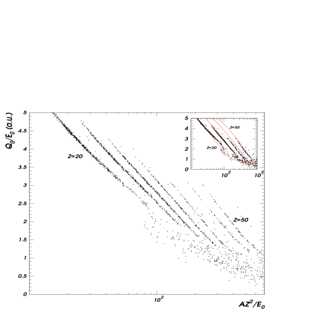
Figure 1: Experimental light efficiency versus the estimate of the average specific electronic stopping power, for different fragments ($\Delta Z=5$). Data from Xe + Sn system at 32 and 50 AMeV [1]. The discrete loci are the effect of the $\delta$ – rays. Its description in the framework of the present scintillation model - solid lines - is compared to the experimental data in the upper box ($\Delta Z=10$).

The above mentioned discrete functions have been interpreted as a signature of modestly energetic ($\approx$ 1 keV) knock-on electrons, the alternative term for $\delta$ - rays, whose ranges exceed the radius $r_{c}$ of the high carrier concentration column along the wake of the ionizing particle, estimated to be around 40 nm [12]. The differential light output per unit path length is the sum of two contributions: one from the highly ionized primary column and one from the knock-on electrons. Considering the total specific electronic stopping power of the incident particle: $(-\d E/\d x)_{e}=(-\d E/\d x)_{p}+(-\d E/\d x)_{\delta}$ as the sum of the energy deposited inside the primary column $(-\d E/\d x)_{p}$ and the energy carried off by the $\delta$ - rays $(-\d E/\d x)_{\delta}$, the fractional energy loss $\cal F$ of the incident particle, deposited outside the primary column, was defined [12]:

$${\cal F}=\frac{(-\d E/\d x)_{\delta}}{(-\d E/\d x)_{e}}.$$ (2)

The differential scintillation efficiency is then given by:

$$\frac{\d{\it L}}{\d E}=(1-{\cal F})\left(\frac{\d{\it L}}{\d E}\right)_{p}+{\cal F}\left(\frac{\d{\it L}}{\d E}\right)_{\delta}.$$ (3)

The scintillation efficiency referring to the primary column $(\d{\it L}/\d E)_{p}$ may be treated with formula (1) provided that $(-\d E/\d x)_{p}$ is known. The $\delta$ – ray scintillation efficiency $(\d{\it L}/\d E)_{\delta}$ is very nearly a constant for energies higher than 1 keV [2, 13]. Estimations of $\cal F$ have shown that this quantity depends only on the energy per nucleon $E/A$ of the particle and it is different from zero only above a certain threshold value $e_{\delta}=(E/A)_{\mathrm{t}hreshold}$ [12]. These characteristics will be found again in the next section in a very simple approach for calculation of $\cal F$, valid for all ions.

Thus, for a particle slowing down in a CsI(Tl) detector from the incident velocity $\propto\sqrt{E_{0}/A}>\sqrt{e_{\delta}}$ to zero, the differential scintillation efficiency is given by Eq. (3) as long as $(E/A)>e_{\delta}$, and by Eq. (1) in the last part of its range, when $(E/A)\leq e_{\delta}$. The total light output would be obtained by integrating the scintillation efficiency over the entire range of the particle. One has to note that the above formulae (1), (3) are not time dependent and consequently they cannot predict the time behaviour of a scintillator signal. In the next section, we shall develop a simple time dependent formalism leading to scintillation efficiency expressions which, up to a supplementary nuclear quenching term, reduces in the first order approximation, to relations very similar to equations (1), (3), when integrated over time.

3 Recombination and nuclear quenching model

3.1 Experimental evidence

The CsI scintillator is an alkali halide crystal having a body centered cubic structure. The present work concerns data from CsI(Tl) operated at room temperature and having a given molar concentration $C\approx 0.02\%-0.2\%$ [14]. The corresponding thallium volume concentration is $N_{A0}\approx 2.11\times 10^{18}-2.10\times 10^{19}$ ions cm^-3. Experimental observations related to the scintillation and its behaviour as a function of temperature in both pure CsI and activated CsI(Tl) crystals can be found in Refs. [7, 15, 16, 17, 18, 19, 20, 21, 22, 23, 24, 25]. In the latter case, the thallium concentration dependence is regarded too. At room temperature, the emission spectrum of a CsI(Tl) excited by charged projectiles [16] is dominated by a broad yellow band, centered near 550 nm.  This band is thus associated with emission from Tl luminescence centres and is referred to as the Tl band [16]. The yellow band nearly completely replaces the competing blue band, related to $I^{-}$ vacancies or elementary colour centres [22, 23] and the ultraviolet (UV) band, considered as an intrinsic property of a perfect crystal [16]. Both of the latter bands are present in case of pure CsI.

We briefly remind the experimental evidence related to CsI(Tl) at a given temperature and concentration, on which our model is dependent. a) The scintillation efficiency is non-linearly increasing with the increasing energy of the particle. For different ions at the same energy, the scintillation efficiency decreases with increasing specific electronic stopping power [7]. If the ionizing particle is an electron or a $\gamma$ – ray of energy higher than 100 keV, the light output may be considered to a good approximation as a linear function of energy [24, 26]. b) The scintillation efficiency depends on the fraction of deposited energy creating $\delta$ – rays [12], which affects the monotonic behaviour resulting from the previous item. c) Combined studies of light efficiency and scintillator decay-constant versus temperature [7, 27] have indicated that the quenching effect is external to the luminescence centre [7].

3.2 The scenario

An ionizing particle excites the scintillator crystal along its path by creating carriers: electrons, promoted in the conduction band, and associated holes in the valence band. CsI(Tl) is an insulator and the energy gap between these two bands is of the order of the mean ionization energy $\epsilon\approx 10$ eV [2]. Thallium iodide is melted with the caesium iodide host bulk before the crystal growth [14]. Some cation sites are occupied by Tl⁺ ions having lost one valence electron in favour of I^- anions. As in the case of KCl(Tl) [28], the excited energy levels of the Tl⁺ ions are presumably localized in the forbidden band of the host lattice. Even though deeper than in the semiconductor case, these levels may essentially participate in the ionized lattice deexcitation, provided that they are free.

Although the emission bands of the CsI(Tl) scintillators, of which the most prevalent one is centred at about 550 nm,  have been intensively studied, there is still controversial discussion about the origin of this band [28, 29, 30, 31, 32, 33, 34, 35, 36, 37, 38, 39, 40]. Thus, according to different interpretations, the luminescence emission may imply, for example, a single thallium centre [31], a couple of Tl⁺ - $V_{k}$ centres [38] or even more complex cluster configurations nearby a Tl impurity [39, 40]. As definitions of the imperfection centres we use those in Ref. [41]. Most of the mentioned approaches converge towards two ideas: for the luminescence induced by highly ionizing particles, both type of carriers, electrons and holes, play a role in the emitted light, i.e. in the scintillation efficiency; the radiative emission around 550 nm  takes place in the $(Tl^{+})^{*}$ excited ions. Let us imagine a formal, oversimplified scenario for the scintillation process, by exemplifying it on the latter luminescence centres.

We suppose that the Tl⁺ ion, with its 2 remaining valence electrons, superfluous in the ionic bond of the CsI lattice, has a donor behaviour. Stimulated by thermal vibrations, the Tl⁺ ions are loosing, in part, some of the outer electrons, creating intruded levels into the upper part of the forbidden band. These double ionized thallium atoms Tl⁺⁺ would become electron traps of volume concentration $N_{A}$. The remaining Tl⁺ ions would be the hole traps, with the volume concentration $\Delta N_{A}=N_{A0}-N_{A}$. One could reason as following: in the highly ionized fiducial volume, the holes are mainly trapped, via a mechanism which is disregarded here, by Tl⁺ ions becoming Tl⁺⁺ ions, while the electrons are mainly trapped on excited levels by such newly created double ionized thallium atoms or by previously existing ones due to thermal excitation. They form $(Tl^{+})^{*}$ excited ions which decay afterwards by emitting the scintillation of energy $h\nu$, in the characteristic 550 nm  band; here $h$ is the Planck constant and $\nu$ is the light frequency. The scheme of the process is:

$$Tl^{++}+electron \longrightarrow (Tl^{+})^{*}+h\nu$$

$$Tl^{+}+hole \longrightarrow Tl^{++}.$$

The mathematical formalism is the same if a more complex configuration of the luminescence centre is considered. During the non-equilibrium state in the cylinder around the ionizing particle trajectory, the two states of thallium feed one another via the carrier trapping, closing in this way the cycle which insures the restoration of the equilibrium and the local electrical neutrality. A time dependent formalism which treats the kinetics of the volume concentrations for both types of carriers and thallium traps would somehow cover also the “exciton” scenario [2, 7, 37, 38, 39, 40]. In this way, it would not be necessary to isolate in time the two steps of the scintillation process: prompt formation of exciton and its delayed deexcitation.

Similarly to the levels created by thallium impurities, deeper levels may be intruded by other point defects of the crystal: the cations and anions removed towards interstitial positions, or for the pure alkali halides more probably to the crystal surface [21], and the associated vacancies. The positive and negative defects are produced by thermal vibrations in practically equal concentrations $N_{D}$ [21]. These levels may compete with the activator sites in carrier trapping, following radiative transitions in the blue band or non-radiative transitions. In insulators, the Fermi-Dirac statistics of the carrier states is well approximated by a Boltzmann function. The concentration of those carriers located at the defect sites, together with the neutrality condition [42], provide the defect distribution, described by a Boltzmann function too. The energy of a nearest-neighbour bound in a solid is of the order of 1 eV. Actually, after Kittel [21], the cation and anion defect concentrations are $N_{D}\approx N_{H}\times\exp(-W_{D}/k{\cal T})$, where $N_{H}$ is the host volume concentration of cations and anions and $W_{D}\approx 1$eV is much larger than the mean vibrational energy. Comparable values for $W_{D}$ (0.2 - 0.4 eV) are obtained with the above expression from concentration of elementary colour centres of the order of 10¹⁵ - 10¹⁸ centres cm^-3, determined by means of absorption coefficients [41]. In a Boltzmann type distribution, $N_{D}$ would represent the number of cations or anions per unit volume having energies higher than $W_{D}$. Consequently, $W_{D}\approx$ 1 eV would be the minimum energy, transferred to a lattice ion, required to produce a defect. At a given temperature, the number of defects may be enhanced by the nuclear interaction of the incident particle with the lattice nuclei. This interaction is proportional to the specific nuclear stopping power $-(\d E/\d x)_{n}=S_{n}$ and produces an additional defect concentration (practically the same for cations and anions) $N_{n}$.

Besides, one has to consider the capture of electrons by the ionized atoms in the wake of the particles, i.e. the “direct” electron-hole recombination, leading to the crystal intrinsic transitions in the UV band. This process probability increases with the specific electronic stopping power $-(\d E/\d x)_{e}=S_{e}$ of the incident particle, while it has to be practically null for electrons. In experiments, a small UV peak was observed for the heaviest ions of low energy. On the contrary, for very energetic protons punching out through a thin CsI(Tl) crystal, in such a way that the Bragg peak is not contributing to the scintillation, both quantities $S_{e}$ and $S_{n}$ are so weak that the shape of their signal is nearly similar to that of electrons generated by $\gamma$ – rays. We do not consider the possible feeding of the yellow band by scintillations in UV band, a two step process in CsI(Tl) put in evidence by UV laser irradiation [43].

By quantifying these assumptions, it will be possible to account for the main experimental observations mentioned by items a) – c) of the subsection 3.1.

3.3 Stopping powers

An incident fragment slowing in a CsI(Tl) crystal loses its energy mostly by ionization, and in a much smaller fraction, by interacting with the nuclei of the lattice. The specific energy loss is $-(\d E/\d x)=S_{e}+S_{n}=S_{e}(1+S_{n}/S_{e})$, the sum of the specific electronic and nuclear stopping powers, expressed in eV$\times 10^{-15}$ atoms^-1 cm². Multiplied by the crystal density $\rho$, they lead to the corresponding stopping powers per unit length: $\rho\times S_{\mathrm{e},n}$, expressed in MeVcm^-1. For the calculation of the differential light output, connected to the differential deposited energy, we have used the stopping powers of Ziegler [44], derived from master curves of $\alpha$ particles, based on Bethe-Bloch formula. For the specific electronic stopping power $S_{e}$ at energies above 2.5 AMeV, an effective charge $Z_{eff}=Z\times\gamma_{eff}(E,A,Z)$ has been used with the parameterization of Hubert et al. for $\gamma_{eff}(E,A,Z)$ [45]. Below 2.5 AMeV, the parameterization of Ziegler was chosen for $\gamma_{eff}(E,A,Z)$ renormalized at 2.5 AMeV, but not lower than 200 AkeV, where $\gamma_{eff}(E,A,Z)$ was kept constant, at the value reached at 200 AkeV: $\gamma_{eff}(E=200$ $A{\mathrm{k}eV},A,Z)$, for each type of fragment. At the atomic number $Z$, the integer of $A=2.072Z+2.32\times 10^{-3}Z^{2}$ for $Z<50$ or $A=2.045Z+3.57\times 10^{-3}Z^{2}$ for $Z\geq 50$ [46] is used as mass number [1]. The resulting $S_{e}$ curves vs the energy per nucleon $E/A$ are plotted - with solid lines - in Fig. 2a), for several atomic numbers. The corresponding specific nuclear stopping powers, as calculated by Ziegler’s approach [44], are shown in Fig. 2b) - solid lines.

In order to determine ${\cal F}(E)$ in the next subsection, we introduce, besides the specific electronic stopping power $(-\d E/\d x)_{e}$, the restricted mean rate of specific electronic energy loss $(-\d E/\d x)_{T<T_{\mathrm{c}ut}}$ [48], which is the mean rate of energy deposited for collisions excluding energy transfers $T$ to electrons greater than a cut off value $T_{\mathrm{c}ut}$. In this case, we have preferred analytical expressions of these quantities instead of the above mentioned Ziegler recipe which is used later for calculating light output and which is not easily to handle. These are based on Bethe-Bloch expressions that are valuable for moderately relativistic charged particles ($E/A\geq 80MeV/u$ for the CsI medium), other than electrons [48], with the parametrization $I=16Z_{\mathrm{M}}^{0.9}$ for the ionization “constant” [49]. By grafting on these expressions the effective charge defined above $Z_{eff}=Z\gamma_{eff}$, the lower limit of their domain of applicability goes down towards 1 - 2 MeV/u, as shown by the dashed curves in Fig. 2a) for $(-\d E/\d x)_{e}$.

The elastic Coulomb scattering on the crystal lattice nuclei - the main part of the nuclear interaction and hence of the specific nuclear stopping power - is used to quantify the density of lattice defects induced by the incident particle: $N_{\mathrm{R}uth}=(\rho{\cal N}_{\mathrm{A}}/(\langle A_{\mathrm{C}sI}\rangle\times\pi r_{c}^{2}))\int_{\theta^{\prime}_{\mathrm{m}in}}^{\pi}(d\sigma^{\prime}/d\Omega^{\prime})d\Omega^{\prime}$. Here $\langle A_{\mathrm{C}sI}\rangle=129.905$ g is the mean atom-gram, $\cal N_{A}$ is Avogadro’s number and (${\mathrm{d}}\sigma^{\prime}/{\mathrm{d}}\Omega^{\prime}$) is the Rutherford cross section in the centre of mass (c.m.) frame; the minimum deflection angle in the c.m. frame $\theta^{\prime}_{min}$, necessary to transfer an energy $\delta E=W_{D}$ in one Coulomb deflection event, may be calculated in classical kinematics from the latter equality if the energy required to produce a defect in the lattice $W_{D}$ is known. Then:

$$N_{\mathrm{R}uth}\propto\left(\frac{\langle Z_{CsI}\rangle}{\langle A_{CsI}\rangle}\right)^{2}\frac{AZ^{2}}{E}\left[\frac{2}{W_{D}}-\frac{\langle A_{CsI}\rangle}{2AE}\left(1+\frac{A}{\langle A_{CsI}\rangle}\right)^{2}\right],$$ (4)

where $\langle Z_{CsI}\rangle=54$ is the average atomic number of the CsI medium. $N_{\mathrm{R}uth}$, the simple, analytical alternative to the volume concentration $N_{n}\propto S_{n}$, is plotted in Fig. 2b) for $W_{D}=1eV$; the different atomic number curves are practically superposed - dashed line. In the same figure, the first term of the above equation $\propto AZ^{2}/E$, weighted also by $1/Z^{2}$, was represented with a dotted line. This result provides a good approximation to $N_{\mathrm{R}uth}$.

Figure 2: Specific energy loss divided by $Z^{2}$ for different ions ($\Delta Z=10$) in CsI(Tl), versus the energy per nucleon. a) Specific electronic stopping power as in Refs. [44, 45] - solid lines; approximate specific electronic stopping power used in calculation of $\cal F$ - dashed lines. b) Specific nuclear stopping power as in Ref. [44] - solid lines. The dashed curves concerning the density of lattice ions displaced by Coulomb scattering (Eq. (4) for $W_{D}=1eV$) are indistinguishable for all ions, and well approximated by the first term of the mentioned formula - dotted line. For a) and b), see subsection 3.3 for explanations.

3.4 Calculation of ${\cal F}$

The discrete functions in Fig. 1 can not be explained in terms of the carrier diffusion process only. Let us suppose that there is a carrier concentration threshold, below which quenching does not exist. The solution of a diffusion equation in cylindrical geometry predicts a concentration which diminishes with time and with the radial distance, but remains proportional to the initial density of carriers per unit length of the ion track. This fact may be only compatible with a monotonic decrease of the light output with the stopping power and not with the discrete functions mentioned above. In addition, the transverse outflow of the carriers is somehow inhibited by space charge effects. A very high carrier concentration is maintained in the proximity of the incident particle path [47]. Consequently, the diffusion is not taken into consideration in the next calculation. On the other hand, we have seen in subsection 2.2 that this dependence is compatible with the knock-on electron generation. These electrons have ranges greater than $r_{c}$, viz. energies higher than a cut off value $T_{cut}$, taking with them a fraction ${\cal F}(E)$ of the energy deposited in the path element $\d x$.

If $\beta$ and $\gamma$ are the kinematic variables of the incident particle, $c$ is the speed of light in vacuum and $u$ the unified atomic mass unit, the maximum energy $T_{max}$ which may be transferred to a stationary unbound electron of mass $m_{\mathrm{e}}$ may be calculated as $T_{\mathrm{m}ax}=2m_{\mathrm{e}}c^{2}\beta^{2}\gamma^{2}$ in the “low energy” approximation $2\gamma m_{\mathrm{e}}/(A\times u)\ll 1$ [48]. The condition that such an electron escapes the primary column and can be considered as a $\delta$ - ray is that this energy is at least equal to $T_{cut}$; otherwise said:

$$T_{max}\geq T_{cut}=2m_{\mathrm{e}}c^{2}\beta_{\delta}^{2}\gamma_{\delta}^{2},$$ (5)

where the index $\delta$ at the kinematic variables refers to the minimum energy per nucleon $e_{\delta}$ of the incident particle that still generates $\delta$ – rays ($\beta_{\delta}^{2}\approx 2e_{\delta}/(uc^{2})$ in the non-relativistic approximation). $(-\d E/\d x)_{T<T_{\mathrm{c}ut}}$, defined in the previous subsection, provides the specific electronic stopping power deposited inside the primary column. The energy deposited by the $\delta$ - rays outside the primary column is $(-\d E/\d x)_{\delta}=(-\d E/\d x)_{e}-(-\d E/\d x)_{T<T_{\mathrm{c}ut}}$. From Eq. (2), the factor $\cal F$ becomes in this case:

$${\cal F}=\frac{(-\d E/\d x)_{\delta}}{(-\d E/\d x)_{e}}=\frac{1}{2}\frac{\ln(\frac{T_{\mathrm{m}ax}}{T_{\mathrm{c}ut}})-\beta^{2}+\beta^{2}\frac{T_{\mathrm{c}ut}}{T_{\mathrm{m}ax}}}{\frac{1}{2}\ln(\frac{2m_{\mathrm{e}}c^{2}\beta^{2}\gamma^{2}}{I^{2}}T_{\mathrm{m}ax})-\beta^{2}-\frac{\Delta}{2}},$$ (6)

($\Delta$ being the density effect in Bethe-Bloch formula [48]), which in the nonrelativistic approximation $\beta^{2}\ll 1$ reads:

$${\cal F}\approx\frac{1}{2}\frac{\ln(\frac{\beta^{2}}{\beta_{\mathrm{\delta}}^{2}})}{\ln(\frac{2m_{\mathrm{e}}c^{2}}{I}\beta_{\mathrm{\delta}}^{2})+\ln(\frac{\beta^{2}}{\beta_{\mathrm{\delta}}^{2}})}.$$ (7)

Eq. 7 is valuable only for $\beta\geq\beta_{\delta}$, under this limit $\cal F$ is zero. The only unknown quantity in the expression of $\cal F$ is $e_{\delta}$, which will be one of the free parameters of the model. The factor $\cal F$ vs $E/A$ is plotted in Fig. 3a) for different threshold energy per nucleon $e_{\mathrm{\delta}}$ values.

Figure 3: a) The fractional energy loss $\cal F$ carried outside the primary column by the $\delta$ – rays; it depends on the fragment velocity $\propto\sqrt{E/A}$, but not on its identity (Eq. (7)). Different curves correspond to different hypothetical values of $T_{cut}$, the cut off value in the electron energy above which they may be considered as $\delta$ - rays escaping the highly ionized fiducial cylinder of radius $r_{c}$ along the fragment wake. b) $T_{cut}$ - solid line - and $r_{c}$ - dashed line - against the fragment energy per nucleon threshold necessary to generate $\delta$ – rays.

3.5 Estimation of $r_{\mathrm{c}}$

One may calculate, from equation (5), the minimum $\delta$ – ray energy values $T_{\mathrm{c}ut}$ required to escape the primary column, as a function of $e_{\mathrm{\delta}}$. In the knock-on electron energy interval of interest here, it is found experimentally that the practical [12] range - energy relation can be reasonably described in various stopping media by a function of the form: $R_{\mathrm{e}}=bT^{n}$ [50], where both b and n are constants [51, 52]. With $R_{\mathrm{e}}$ in mg cm^-2 and $T$ in keV, and considering CsI as having an intermediate mean atomic number between those of aluminium and gold, the two extreme media treated in Refs. [51, 52], we find the particular value b = 0.016 by keeping n=1.35 [12, 51] as universal power index for all the stopping media. Consequently, and without taking into account the angular distribution of the scattered $\delta$ – rays, one may estimate the corresponding primary column radius $r_{\mathrm{c}}$. Both quantities: $T_{cut}$ and $r_{c}$ are plotted in Fig. 3b) versus $e_{\delta}$.

3.6 The formalism

Inside the primary column, the initial (t=0) volume concentrations of the created pair carriers: electrons (e) and holes (h), at the coordinate $x$ along the particle path, are proportional to the electronic stopping power per unit length $\rho S_{e}$:

$$n_{\mathrm{h}}(x,0)=n_{\mathrm{h}_{0}}(x) = \frac{\rho S_{\mathrm{e}}(x)}{\epsilon\pi r_{\mathrm{c}}^{2}}=n_{0}(x)$$ (8)

$$n_{\mathrm{e}}(x,0)=n_{\mathrm{e}_{\mathrm{0}}}(x)=\left(1-{\cal F}(x)\right)\frac{\rho S_{\mathrm{e}}(x)}{\epsilon\pi r_{\mathrm{c}}^{2}} = \left(1-{\cal F}(x)\right)n_{0}(x)$$ (9)

for holes and electrons, respectively. The number of knock-on electrons per unit length escaping out of the primary column (as long as $E/A>e_{\delta}$) is ${\cal F}\rho S_{\mathrm{e}}/\epsilon$ ($\epsilon$ being the mean ionization energy). They will produce other ionizations outside the primary column. The radial diffusion is not treated here.

The basic assumptions concerning the thallium activator centres in the caesium iodide crystal is that they may exist in two different states: one acting as hole trap - of concentration $\Delta N_{A}$ - and the other one - of concentration $N_{A}$ - which acts as electron trap, to produce afterwards the scintillation.

The excited system inside the primary column has the tendency to come back to the equilibrium state. The electrons may be trapped by thallium electron traps with a probability $\Lambda_{\mathrm{A}e}N_{\mathrm{A}}$, or by defects with a probability $\Lambda_{\mathrm{D}e}\left(N_{\mathrm{D}}+N_{\mathrm{n}}\right)$, or they may directly recombine with holes at ionized cation and anion sites of the lattice, with a probability $\Lambda_{\mathrm{R}}n_{\mathrm{h}}\left(x,t\right)$. The holes, in their turn, may be trapped by the thallium hole traps with a probability $\Lambda_{\mathrm{A}h}\Delta N_{\mathrm{A}}$, or by defects, with a probability $\Lambda_{\mathrm{D}h}\left(N_{\mathrm{D}}+N_{\mathrm{n}}\right)$ or they may recombine with the electrons, with a probability $\Lambda_{\mathrm{R}}n_{\mathrm{e}}\left(x,t\right)$. The equations concerning the time variation of the carrier concentrations inside the primary column read:

$$-\frac{\d n_{\mathrm{e}}(x,t)}{\d t} = \left[\Lambda_{\mathrm{A}e}N_{\mathrm{A}}+\Lambda_{\mathrm{D}e}\left(N_{\mathrm{D}}+N_{\mathrm{n}}\right)\right]n_{\mathrm{e}}(x,t)$$ (10)

$$+ \Lambda_{\mathrm{R}}n_{\mathrm{h}}\left(x,t\right)n_{\mathrm{e}}(x,t)$$

$$-\frac{\d n_{\mathrm{h}}(x,t)}{\d t} = \left[\Lambda_{\mathrm{A}h}\Delta N_{\mathrm{A}}+\Lambda_{\mathrm{D}h}\left(N_{\mathrm{D}}+N_{\mathrm{n}}\right)\right]n_{\mathrm{h}}(x,t)$$ (11)

$$+ \Lambda_{\mathrm{R}}n_{\mathrm{e}}\left(x,t\right)n_{\mathrm{h}}(x,t).$$

By disregarding the activator centre depletion [24], the coefficients $\Lambda_{\mathrm{A}e}N_{\mathrm{A}}$ and $\Lambda_{\mathrm{A}h}\Delta N_{\mathrm{A}}$ may be considered as being approximately constant. For the sake of simplicity, we make the same hypothesis for $\Lambda_{\mathrm{D}e}\left(N_{\mathrm{D}}+N_{\mathrm{n}}\right)$ and $\Lambda_{\mathrm{D}h}\left(N_{\mathrm{D}}+N_{\mathrm{n}}\right)$. In this way, we must solve two coupled first order differential equations with constant coefficients. The initial conditions are given by the expressions (8,9), where ${\cal F}>0$ for $E/A>e_{\mathrm{\delta}}$ and ${\cal F}=0$ for $E/A\leq e_{\mathrm{\delta}}$. Of course the number of defects is much smaller than that of the activator centres, but we shall see in the next section that the nuclear induced defects play a role in describing the total light output at lower incident energies. In order to keep the number of free parameters in the resulting fit procedure as low as possible, we make the hypotheses that: $\Lambda_{\mathrm{D}h}\approx\Lambda_{\mathrm{D}e}=\Lambda_{\mathrm{D}}$. Our tests have shown that the ratio $(\Lambda_{\mathrm{A}h}\Delta N_{\mathrm{A}}+\Lambda_{\mathrm{D}}N_{\mathrm{D}})/(\Lambda_{\mathrm{A}e}N_{\mathrm{A}}+\Lambda_{\mathrm{D}}N_{\mathrm{D}})\approx 1$ and that the shape of the total light output is not critically sensitive to its magnitude around this value. Thus, instead of keeping this ratio as a free fit parameter, we fix its value at 1. We make the notations: $\Lambda^{\prime}_{\mathrm{A}e,D,R}=\Lambda_{\mathrm{A}e,D,R}/(\Lambda_{\mathrm{A}e}N_{\mathrm{A}}+\Lambda_{\mathrm{D}}N_{\mathrm{D}})$. Under the above assumptions, one may calculate the first derivative of the hole concentration with respect to the electron concentration:

$$\frac{\d n_{\mathrm{h}}\left(x,t\right)}{\d n_{\mathrm{e}}\left(x,t\right)}=\frac{\left(1+\Lambda^{\prime}_{\mathrm{D}}N_{\mathrm{n}}+\Lambda^{\prime}_{\mathrm{R}}n_{\mathrm{e}}\left(x,t\right)\right)n_{\mathrm{h}}\left(x,t\right)}{\left(1+\Lambda^{\prime}_{\mathrm{D}}N_{\mathrm{n}}+\Lambda^{\prime}_{\mathrm{R}}n_{\mathrm{h}}\left(x,t\right)\right)n_{\mathrm{e}}\left(x,t\right)}.$$ (12)

The carrier concentrations are correlated. At every moment $t$ and position $x$, the hole concentration $n_{\mathrm{h}}\left(x,t\right)$ may be considered as a function of the electron concentration $n_{\mathrm{e}}\left(x,t\right)$, expressed by a Taylor series expansion around the initial value at the $x$ coordinate $n_{\mathrm{e}}\left(x,0\right)=n_{\mathrm{e}_{\mathrm{0}}}$. By keeping only the zero and first order terms in the expansion, viz. by considering that $n_{\mathrm{h}}\left(x,t\right)$ is linearly dependent on $n_{\mathrm{e}}\left(x,t\right)$ and by replacing it in the rate equation for the electron concentration Eq. (10), one may determine the time dependent solution:

$$n_{\mathrm{e}}\left(x,t\right)=$$

$$\frac{p\left(x\right)\left(1-{\cal F}\left(x\right)\right)n_{\mathrm{0}}\left(x\right)}{\left(1+\Lambda^{\prime}_{\mathrm{D}}N_{\mathrm{n}}\left(x\right)+\Lambda^{\prime}_{\mathrm{R}}n_{\mathrm{0}}\left(x\right)\right)\exp\left(p\left(x\right)\left(\Lambda_{\mathrm{A}e}N_{\mathrm{A}}+\Lambda_{\mathrm{D}}N_{\mathrm{D}}\right)t\right)-y\left(x\right)\Lambda^{\prime}_{\mathrm{R}}n_{\mathrm{0}}\left(x\right)}$$

with $p(x)=1+\Lambda^{\prime}_{\mathrm{D}}N_{\mathrm{n}}(x)+\left(1-y(x)\right)\Lambda^{\prime}_{\mathrm{R}}n_{\mathrm{0}}(x)$ in every point $x$ of the ionizing particle trajectory, and $y(x)=1-{\cal F}\left(x\right)\Lambda_{\mathrm{R}}^{\prime}n_{\mathrm{0}}(x)/\left(1+\Lambda_{\mathrm{D}}^{\prime}N_{\mathrm{n}}(x)+\Lambda_{\mathrm{R}}^{\prime}n_{\mathrm{0}}(x)\right)$.

For the $\delta$ – rays, which are supposed to produce new ionizations outside the primary column, the new created carrier concentration equations are completely decoupled for electrons and holes, because there is no radiation damage nor are there recombination processes. In the electron equation of interest, only the first two linear terms (concerning the activator and permanent defect sites) on the right side of the Eq. (10) have to be kept. Thus, the solution will be a simple exponential.

3.7 The light output

The double differential light output $(\d^{2}L(x,t)/\d x\d t)_{p}$ in the primary column is given, within a multiplicative constant “a” (related to the energy - light unit conversion, the light collection in connection to the shape of the crystal and the PMT gain), by the first of the linear terms in equation (10): $a\epsilon\pi r_{c}^{2}\Lambda_{\mathrm{A}e}N_{\mathrm{A}}n_{e}(x,t)$. Integrated over time between $0$ and $\infty$, this term leads to the differential light output in the infinitesimal element $\d x$ of the primary column:

$$\left(\frac{\d L(x)}{\d x}\right)_{\mathrm{p}}=a\epsilon\pi r_{\mathrm{c}}^{2}\Lambda_{\mathrm{A}e}^{\prime}N_{\mathrm{A}}\frac{1-{\cal F}(x)}{y(x)\Lambda_{\mathrm{R}}^{\prime}}\ln\left[\frac{1+\Lambda_{\mathrm{D}}^{\prime}N_{\mathrm{n}}(x)+\Lambda_{\mathrm{R}}^{\prime}n_{\mathrm{0}}(x)}{1+\Lambda_{\mathrm{D}}^{\prime}N_{\mathrm{n}}(x)+\left(1-y(x)\right)\Lambda_{\mathrm{R}}^{\prime}n_{\mathrm{0}}(x)}\right].$$ (14)

The differential light output generated by the $\delta$ – rays in the same infinitesimal element $\d x$ (determined by integrating over time the corresponding exponential solution of electron rate equation) is:

$$\left(\frac{\d L(x)}{\d x}\right)_{\mathrm{\delta}}=a\Lambda_{\mathrm{A}e}^{\prime}N_{\mathrm{A}}{\cal F}(x)\rho S_{\mathrm{e}}=a\epsilon\pi r_{\mathrm{c}}^{2}\Lambda_{\mathrm{A}e}^{\prime}N_{\mathrm{A}}{\cal F}(x)n_{\mathrm{0}}(x).$$ (15)

The total differential light output $(\d L(x)/\d x)$ is the sum of the light produced inside the primary column and outside it. The integration over the range of the particle $R(E_{\mathrm{0}})$ or, by changing the variable, over the energy $E_{0}$ leads to the total light output expression:

$$L = a_{\mathrm{G}}\left[\int^{E_{\delta}}_{0}\frac{1}{a_{\mathrm{R}}S_{\mathrm{e}}(E)}\ln\left(1-\frac{a_{\mathrm{R}}S_{\mathrm{e}}(E)}{1+a_{\mathrm{n}}S_{\mathrm{n}}(E)+a_{\mathrm{R}}S_{\mathrm{e}}(E)}\right)^{-1}\frac{\d E}{1+\frac{S_{\mathrm{n}}(E)}{S_{\mathrm{e}}(E)}}\right.$$ (16)

$$+ \int_{E_{\delta}}^{E_{0}}\frac{1-{\cal F}(E)}{y(E)a_{\mathrm{R}}S_{\mathrm{e}}(E)}\ln\left(1-\frac{y(E)a_{\mathrm{R}}S_{\mathrm{e}}(E)}{1+a_{\mathrm{n}}S_{\mathrm{n}}(E)+a_{\mathrm{R}}S_{\mathrm{e}}(E)}\right)^{-1}\frac{\d E}{1+\frac{S_{\mathrm{n}}(E)}{S_{\mathrm{e}}(E)}}$$

$$+ \left.\int_{E_{\delta}}^{E_{0}}\frac{{\cal F}(E)\d E}{1+\frac{S_{\mathrm{n}}(E)}{S_{\mathrm{e}}(E)}}\right],$$

where $y(E)=1-{\cal F}(E)a_{\mathrm{R}}S_{\mathrm{e}}(E)/(1+a_{\mathrm{n}}S_{\mathrm{n}}(E)+a_{\mathrm{R}}S_{\mathrm{e}}(E))$. This light output expression contains four model parameters: $a_{\mathrm{G}}=a\Lambda_{\mathrm{A}e}^{\prime}N_{\mathrm{A}}\rho$, $a_{\mathrm{R}}=\Lambda_{\mathrm{R}}^{\prime}\rho/\left(\epsilon\pi r_{\mathrm{c}}^{2}\right)$, $a_{\mathrm{n}}=\Lambda_{\mathrm{D}}^{\prime}\rho/\left(\epsilon\pi r_{\mathrm{c}}^{2}\right)\times\left(\epsilon/\epsilon_{\mathrm{n}}\right)$, written like this because $N_{\mathrm{n}}(E)=\rho S_{\mathrm{n}}(E)/\left(\epsilon_{\mathrm{n}}\pi r_{\mathrm{c}}^{2}\right)$ (here, $\epsilon_{\mathrm{n}}$ is the mean energy required to produce a dislocation) and $e_{\delta}$ ($E_{\delta}=A\times e_{\delta}$). These parameters denote meaningful quantities. $a_{\mathrm{G}}$ is the “gain” parameter, related to the energy-light unit conversion, light collection, conversion factor for producing photoelectrons and the electronic gain. $a_{\mathrm{R}}$, $a_{\mathrm{n}}$ are the “recombination quenching” and “nuclear quenching” parameters respectively, related to the processes which divert part of the deposited energy - what we call “quenching”. $e_{\delta}$ is the energy per nucleon above which the $\delta$ – rays play a role in the scintillation mechanism.

The first term in Eq. (16) refers to the last part of the particle range, where the energy has decreased below the $\delta$ – ray production threshold $E\leq A\times e_{\delta}$ and thus ${\cal F}(E)=0$. The last two terms concern the first part of the trajectory ($E>A\times e_{\delta}$ and ${\cal F}(E)>0$) as follows: the second term reports on the light output originating inside the primary column, while the third one is connected to the light produced by the knock-on electrons outside the primary column. For the low incident energies $E_{\mathrm{0}}\leq A\times e_{\delta}$, ${\cal F}(E)=0$ along the entire range of the particle and only the first term will be present.

4 Comparison to the experimental data

4.1 The light output – energy relation

It is possible now to confront the light output - energy relation in Eq. (16) to experimental dependence, provided that the above four coefficients are known. Actually, they are determined, from data concerning ions with $Z\leq 45$, as fit parameters by a $\chi^{2}$ minimization procedure using the MINUIT package from CERN library. The experimental light output values $Q_{\mathrm{0}}$, and the corresponding energy $E_{\mathrm{0}}$ deposited in a CsI(Tl) crystal of INDRA (see the accompanying paper [1]) are used for the comparison. The integral in expression (16) is performed numerically. The resulting fit parameter values are given in Table 1a). The fourth parameter $a_{\mathrm{n}}$ was held constant after a preliminary analysis. Using these values in expression (16), the total light output was recalculated and compared to the experimental $Q_{0}$ values; the results are plotted versus $E_{0}$ in Fig. 4 - solid lines. There is excellent agreement, within 3% for most data, as will be shown later. In the inset of figure, the low energy results are shown and compared to the case where the nuclear quenching term $a_{\mathrm{n}}S_{\mathrm{n}}(E)$ is disregarded (dashed line). The small unrealistic bump of this pure recombination quenching case, induced by the Bragg peak in the specific electronic stopping power $S_{\mathrm{e}}(E)$, is completely eliminated by including $a_{\mathrm{n}}S_{\mathrm{n}}(E)$. Thus, the nuclear quenching term may be considered as a “fine tuning” device allowing a more accurate description of the experimental light output at the lowest energies.

Finally, when fixing $a_{\mathrm{n}}$ at the proposed value (3.9$\times 10^{-1}$ eV${}^{-1}10^{15}$atoms^-1cm²), it is very important to note that light ions up to $Z=7$ are necessary but sufficient to determine the gain parameter $a_{\mathrm{G}}$ to within 10% and the $a_{\mathrm{R}}$ and $e_{\mathrm{\delta}}$ parameters to within 25% of the above mentioned values. If three of the parameters: $a_{\mathrm{n}}$, $e_{\mathrm{\delta}}$ and $a_{\mathrm{R}}$ are fixed at the values listed in Table 1a), the gain parameter $a_{\mathrm{G}}$ is determined to within 2.5% when the experimental data employed in the fit procedure are restricted to light ions $Z\leq 7$ too.

Table 1: Fit parameters: $a_{\mathrm{G}}$, $a_{\mathrm{R}}$, $e_{\mathrm{\delta}}$, $a_{\mathrm{n}}$: gain, recombination quenching, $\delta$ – ray production energy per nucleon threshold and nuclear quenching, respectively, for module 2 of ring 3. The errors on the parameters (one unit on the last digit) are only statistical. For exact calculation (Eq. (16)): a) $N_{\mathrm{n}}\propto S_{\mathrm{n}}$; b) $N_{\mathrm{n}}\approx N_{\mathrm{R}uth}$ and $W_{\mathrm{d}}$ = 1 eV, were assumed. c) Pure recombination case. For the first order approximation calculation (Eq. (18)): d) $N_{\mathrm{n}}\propto S_{\mathrm{n}}$. See subsections 3.7, 4.5 for explanations.

	a)	b)	c)	d)
$a_{\mathrm{G}}$ [a.u.]	20.00	19.94	20.57	18.74
$a_{\mathrm{R}}$ [eV${}^{-1}10^{15}$atoms-1cm2]	2.82$\times 10^{-2}$	2.81$\times 10^{-2}$	3.04$\times 10^{-2}$	1.26$\times 10^{-2}$
$e_{\mathrm{\delta}}$ [MeV$/u$]	1.96	1.95	2.08	1.79
$a_{\mathrm{n}}$ [eV${}^{-1}10^{15}$atoms-1cm2]	3.9$\times 10^{-1}$	4$\times 10^{-1}$ [a.u.]	-	3.9$\times 10^{-1}$

When the defect concentration created by nuclear collisions, instead of being taken as $\propto S_{\mathrm{n}}(E)$, is calculated from the Rutherford diffusion probability - Eq. (4) - the fit parameter values are practically the same (eventually except for $a_{\mathrm{n}}$ because $N_{\mathrm{R}uth}$ may be used in arbitrary units). These values are shown in Table 1b) for $W_{\mathrm{D}}=$1 eV. The light output values calculated in this case are practically identical to those from the previous recipe. Thus, we conclude that the simple expression of $N_{\mathrm{R}uth}$, very well approximated by its first term $\propto AZ^{2}/E$ as shown in Fig. 2b), may be used for the nuclear quenching term estimation. In this case, the value of the fourth parameter $a_{n}$ depends on the value used for $W_{D}$: the smaller $W_{D}$ is, the higher the number of created imperfections (defect or large amplitude vibration levels) and the smaller the determined fit parameter value, and vice-versa. These two quantities cannot be kept simultaneously as free parameters in the fit procedure and one has to choose, for example, a value for $W_{D}$.

In the end, we have to note that the agreement of calculation with data is rather good (except for the lowest energies) even when the nuclear term is disregarded, with the advantage that the number of fit parameters reduces to three. The resulting parameter values are also presented in the Table 1c).

The quality of the above approach, which will be termed the recombination and nuclear quenching model (RNQM) in the following discussion, is illustrated also in the next subsections by three direct consequences.

4.2 The $\delta$ – ray effect

The fraction of the deposited energy ${\cal F}(E)$ transferred to $\delta$ – rays increases with $E/A$ - Fig. 3a), and has the same value irrespective of $Z$. For two different fragments having the same average stopping power $\propto AZ^{2}/E_{\mathrm{0}}$, the higher Z fragment has a higher energy per nucleon, a higher ${\cal F}(E)$ value and, consequently, a higher experimental efficiency $Q_{\mathrm{0}}/E_{\mathrm{0}}$, as shown by symbols in Fig. 1. The calculated scintillation efficiency $L/E_{\mathrm{0}}$ provided by RNQM shows the same behaviour. The total light output is given by expression (16), with the nuclear quenching term $a_{\mathrm{n}}S_{\mathrm{n}}(E)$ or $a_{\mathrm{n}}N_{\mathrm{R}uth}(E)$ (for $W_{\mathrm{D}}=$ 1 eV - 1 keV). The results are shown by the curves in the upper box of Fig. 1 for a few of the heavier fragments, where the effect is quite pronounced. As long as the average specific electronic stopping power is not too high, they qualitatively follow the experimental data. In the latter domain, the curves are increasing when the nuclear quenching term is neglected.

4.3 Reaction product identification in a Si - CsI(Tl) map

At forward angles (rings 2 - 9), the INDRA array is composed of three detection layers: ionisation chamber, 300 $\mu$m thick silicon detector (Si) and CsI(Tl) scintillator. The reaction products cover a large range in energy and atomic number and they can be well identified in a $\Delta E_{\mathrm{S}i}-Q_{\mathrm{0}}$ map - symbols in Fig. 5 - where $\Delta E_{\mathrm{S}i}$ is the energy lost in the silicon detector. With the values of the fit parameters $a_{\mathrm{G}}$,$a_{\mathrm{R}}$,$a_{\mathrm{n}}$,$e_{\mathrm{\delta}}$ in column a) of Table 1 and the expression (16) for the light output, a $\Delta E_{\mathrm{S}i}-L$ map was calculated - solid lines in Fig. 5. The cases b), c) of Table 1 give results practically identical to the case a). The calculated curves have excellent agreement with the experimental loci, within $\Delta Z\approx 1$ for $Z\approx 50$.

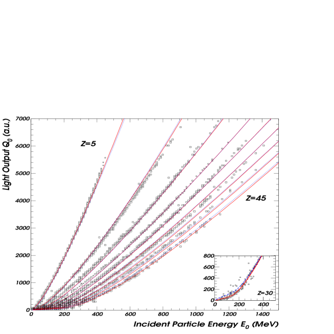
Figure 4: Total light output $Q_{0}$ against the initial particle energy $E_{0}$ for different ions ($\Delta Z$ = 5): the symbols are experimental data from the system Xe + Sn at 32 and 50 AMeV [1], the solid lines are exact calculation (Eq. (16)) and the dotted lines are first order approximation calculation (Eq. (18)). Inset: zoom at low energies; comparison to the case where the nuclear quenching term would be neglected (dashed line) for $Z=30$.

4.4 Energy determination

Having determined the four fit parameters, we may recalculate by Newton iterative method starting from $Q_{\mathrm{0}}$, the incident energy $E_{\mathrm{c}alc}$ of the reaction product, to be compared to the true energy $E_{\mathrm{0}}$. For most of the data, the relative deviation of the calculated energy versus the true energy per nucleon is less than 3% - as shown in Fig. 6a) for several ions with $5\leq Z\leq 50$. Only at low energies $E\leq 5$ AMeV, the discrepancy reaches rather large values: 5% - 10%, and up to 15% in the worst cases - see Fig. 6b). Note that this roughly corresponds to the true energy accuracy, shown by the regions between the two solid lines in Fig. 6a) [1].

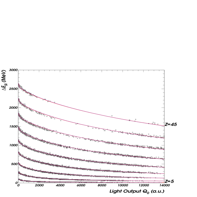
Figure 5: A $\Delta E_{Si}-Q_{0}$ map (module 2, ring 3 of INDRA) from the sytem Xe + Sn at 32 and 50 AMeV. Conventions of presentation are the same as in Fig. 4.

These results are arguments in favour of the present “quenching” model which accounts for the main experimental evidence concerning the scintillation yield of the CsI(Tl) crystals in the yellow band of interest. The ratio $a_{\mathrm{R}}/a_{\mathrm{n}}$ could give an idea of the weights of the two processes: recombination and nuclear quenching, provided that the ratio of the mean energy required to displace a lattice ion from its site to the mean ionization energy $\epsilon_{\mathrm{n}}/\epsilon$ is known.

Figure 6: Deviations (in %) of the energy values determined with Eq. (16) from the true energy values for several products of the reactions Xe + Sn at 32 and 50 AMeV: a) deviations plotted against the product energy per nucleon: symbols; the regions between curves show the accuracy of the true energy per nucleon (see subsection 2.2 of the accompanying paper [1] for details); b) deviation histograms.

The parameter $e_{\mathrm{\delta}}\approx 2$ MeV$/u$, found by the fit procedure, to which corresponds a minimum energy of 4.4 keV for the $\delta$ – rays, allows to roughly estimate - as proposed in subsection 3.5 - the radius of the primary column $r_{\mathrm{c}}\approx$260 nm.  This value is one order of magnitude greater than it has been found in Ref. [12]. Ref. [47] estimates the same quantity in Si to be $1.15\mu$m, with the connected $\delta$ - ray energy $\approx 10$ keV. For electrons having this energy, the range in CsI is of about 770 nm,  of the same order of magnitude as the value found in the present work. The $r_{\mathrm{c}}$ results are given in Table 2. By means of the estimated value $r_{\mathrm{c}}\approx$260 nm,  one may determine the order of magnitude of the carrier concentration $n_{0}$ generated inside the strongly ionized cylinder. For energies 5 $\leq$ E $\leq$ 80 AMeV, one finds $10^{15}\leq n_{0}\leq 10^{18}$ carriers cm^-3 when $2\leq Z\leq 50$, i.e. $n_{0}\leq N_{A0}$. This fact a posteriori supports disregarding activator centre depletion.

Table 2: Estimation of the radius $r_{\mathrm{c}}$ of the transverse area of the primary column: a) Ref. [12], b) present work c) Ref. [47].

	a) Ref. [12]	b) Present work	c) Ref. $\cite[cite]{[\@@bibref{}{sei73}{}{}]}^{*}$
$r_{\mathrm{c}}$ [nm]	40	260	770

^∗ extracted from data in Si

4.5 The first order approximation of the light output expression

The quenching terms in Eqs. (14) for the differential light output and (16) for the total light output were evaluated by means of the parameter values from Table 1a) and stopping powers in the domain of our experimental data: $a_{\mathrm{n}}S_{\mathrm{n}}<a_{\mathrm{R}}S_{\mathrm{e}}\ll 1$. In the first order approximation of the logarithm, the differential light output in the primary column becomes:

$$\left(\frac{\d L(x)}{\d x}\right)_{\mathrm{p}}\approx a_{\mathrm{G}}\frac{1-{\cal F}(x)}{1+a_{\mathrm{n}}S_{\mathrm{n}}(x)+a_{\mathrm{R}}S_{\mathrm{e}}(x)}S_{\mathrm{e}}(x).$$ (17)

In the low energy case $E_{\mathrm{0}}\leq A\times e_{\mathrm{\delta}}$ for which ${\cal F}(x)=0$, the above expression is, except the nuclear term, identical with the formula of Birks [7] from subsection 2.1. In the same approximation, the total light output reads:

$$L = a_{\mathrm{G}}\left[\int^{E_{\delta}}_{0}\frac{1}{1+a_{\mathrm{n}}S_{\mathrm{n}}(E)+a_{\mathrm{R}}S_{\mathrm{e}}(E)}\times\frac{\d E}{1+S_{\mathrm{n}}(E)/S_{\mathrm{e}}(E)}\right.$$ (18)

$$+ \int_{E_{\delta}}^{E_{0}}\frac{1-{\cal F}(E)}{1+a_{\mathrm{n}}S_{\mathrm{n}}(E)+a_{\mathrm{R}}S_{\mathrm{e}}(E)}\times\frac{\d E}{1+S_{\mathrm{n}}(E)/S_{\mathrm{e}}(E)}$$

$$+ \left.\int_{E_{\delta}}^{E_{0}}\frac{{\cal F}(E)\d E}{1+S_{\mathrm{n}}(E)/S_{\mathrm{e}}(E)}\right].$$

The resulting fit parameter values are given in Table 1d). The quality of the results (total light output, fragment identification) obtained in the first order approximation is very close to that achieved by means of the exact treatment, as shown in Figs. 4, 5 – dotted lines. Formula (18), as well as expression (4) in the mentioned approximate form, will allow the analytical integration of the total light output, useful for the applications presented in section 4 of the accompanying paper [1].

5 Conclusions

The nonlinear response of CsI(Tl) was quantified in terms of the competing deexcitation transition probabilities of the excited fiducial volume around the path of a strongly ionizing particle. A simple mathematical formalism was developed to determine total light output based on a numerically integrable, four-parameter dependent expression. The formalism has allowed the inclusion of energetic knock-on electrons. Consequently, their effect in the scintillation efficiency was quantitatively taken into account, in a fully consistent way, for the first time. By a fit procedure, the values of the four parameters were determined. Of physical interest is the energy per nucleon threshold for producing $\delta$ – rays by the incident particle, $e_{\mathrm{\delta}}=2$ MeV$/u$. This result also allows the rough estimation of the primary column radius $r_{\mathrm{c}}$=260 nm  along the wake of the ionizing particle. The predictive character of the model was verified by using telescope-type ($\Delta E_{\mathrm{S}i}-Q_{0}$) reaction product loci data, the agreement calculation - experimental data being within $\Delta Z\approx 1$ for $Z\approx 50$, as well as by using deposited energy data, in the range 1 - 80 AMeV. A comparison of the model predictions to the latter experimental data resulted in variations of the order of the CsI(Tl) scintillator resolution $\approx 3\%$, and within 10% – 15% when the reference energy was known with only a comparable, poorer precision. The effect of the $\delta$ – rays in the scintillation efficiency as a function of the average stopping power in the entire range is quite well described too. In fact, the knock-on electrons play an important role in the light output, especially for heavy reaction products. In the accompanying paper [1], an approximate but analytically integrable formula will be derived from the proposed formalism. Up to now, it was used for rapid calibration and identification procedures in the INDRA 4$\pi$ array. In the future, in relation with computer capabilities, we will use the exact formula proposed here.

References

- [1] M. Parlog et al., Nucl. Instr. and Meth. A, accompanying paper
- [2] A. Meyer and R. B. Murray, Phys. Rev. 122 (1961) 815.
- [3] M. L. Halbert, Phys. Rev. 107 (1957) 647.
- [4] S. Bashkin, R. R. Carlson, R. A. Douglas and J. A. Jacobs, Phys. Rev. 109 (1958) 434.
- [5] A. R. Quinton, C. E. Anderson and W. J. Knox, Phys. Rev. 115 (1959) 886.
- [6] J. B. Birks, Scintillation counters, Pergamon Press (1960) 93.
- [7] J. B. Birks, The theory and practice of scintillation counters, Pergamon Press (1964) 439.
- [8] E. De Filippo et al. Nucl. Instr. and Meth. in Phys. Res. A 342 (1994) 527.
- [9] D. Horn et al., Nucl. Instr. and Meth. A 320 (1992) 273.
- [10] E. Newman and F. E. Steigert, Phys. Rev. 118 (1960) 1575.
- [11] E. Newman, A. M. Smith and F. E. Steigert, Phys. Rev. 122 (1961) 1520.
- [12] A. Meyer and R. B. Murray, Phys. Rev. 128 (1962) 98.
- [13] C. D. Zerby, A. Meyer and R. B. Murray, Nucl. Instr. and Meth. 12 (1961) 115.
- [14] BDH-Merck Ltd, West Quay Rd, Poole, BH15 1HX, England.
- [15] J. C. Robertson, J. G. Lynch and W. Jack, Proc. Phys. Soc. 78 (1961) 1188.
- [16] R. Gwin and R. B. Murray, Phys. Rev. 131 (1963) 508.
- [17] Z. L. Morgenstern, Opt. i Spektroskopia 8 (1960) 672; 7 (1959) 231. (translations: Opt. Spectry. (USSR) 8 (1960) 355; 7 (1959) 146).
- [18] H. Besson, D. Chauvy and J. Rossel, Helv. Phys. Acta 35 (1962) 211.
- [19] J. Bonanomi and J. Rossel, Helv. Phys. Acta 25 (1952) 725.
- [20] H. Knoepfel, E. Leopfe and P. Stoll, Helv. Phys. Acta 30 (1957) 521.
- [21] Charles Kittel, Introduction to solid state physics, third edition, John Wiley and Sons, Inc. (1966) 563.
- [22] P. Schotanus, R. Kamermans and P. Dorenbos, IEEE Trans. Nucl. Sci. NS-37 (1990) 177.
- [23] J. D. Valentine, W. M. Moses, S. E. Derenzo, D. K. Wehe and G. F. Knoll, Nucl. Instr. and Meth. A 325 (1993) 147.
- [24] R. Gwin and R. B. Murray, Phys. Rev. 131 (1963) 501.
- [25] F. S. Eby and W. K. Jentschke, Phys. Rev. 96 (1954) 911.
- [26] B. D. Rooney and J. D. Valentine, IEEE Trans. Nucl. Sci. 44 (1997) 509.
- [27] Van Sciver and L. Bogart, I.R.E. Trans. Nucl. Sci. NS-3 (1958) 90.
- [28] P. D. Johnson and F. E. Williams, J. Chem. Phys. 21 (1953) 125.
- [29] A. I. Popov, S. A. Chernov and L. E. Trinkler, Nucl. Instr. and Meth. B 122 (1997) 602.
- [30] S Masunga, I. Morita and M. Ishiguro, J. Phys. Soc. Japan 21 (1968) 638.
- [31] S. E. Derenzo, M. J. Weber,Nucl. Instr. and Meth. A 422 (1999) 111.
- [32] V. B. Gutan, L. M. Shamovskii, A. A. Dunina and B. S. Gorobets, Opt. Spectrosc. 37 (1974) 407.
- [33] R. G. Kaufman, W. B. Hadley and H. N. Hersh, IEEE Trans. Nucl. Sci NS-17 (1970) 82.
- [34] R. B. Murray, IEEE Trans. Nucl. Sci. NS-22 (1975) 54.
- [35] K. Michaelian and A. Menchaca-Rocha, Phys. Rev. B 49 (1994) 15550.
- [36] K. Michaelian, A. Menchaca-Rocha, E. Belmont-Moreno, Nucl. Instr. and Meth. A 356 (1995) 297.
- [37] L. P. Smol’skaya and T. A. Koesnikova, Opt. Spectrosc. 47 (1979) 292.
- [38] J. M. Spaeth, W. Meise and K. S. Song, J. Phys. Condens. Matter. 6 (1994) 3999.
- [39] V. Nagirnyi, S. Zazubovich, V. Zepelin, M. Nikl, G. P. Pazzi, Chem. Phys. Lett. 227 (1994) 535.
- [40] V. Nagirnyi, A. Stolovich, S. Zazubovich, V. Zepelin, E. Mihokova, M. Nikl, G. P. Pazzi, L. Salvini, J. Phys. Condens. Matter 7 (1995) 3637.
- [41] A. S. Marfunin, Spectroscopy, luminescence and radiation centers, Springer-Verlag, Berlin Heidelberg New York, 1979.
- [42] C. Constantinescu, Lecture course in solid state physics, Bucharest University (1970); C. Constantinescu and Gh. Ciobanu, Solid State Physics, vol.I, Technical Press, Bucharest.
- [43] J. Pouthas et al., Nucl. Instr. and Meth. A 357 (1995) 418.
- [44] J. F. Ziegler, Helium Stopping Powers and Ranges in All Elements, Pergamon, New York (1977).
- [45] F. Hubert, R. Bimbot, H. Gauvin, At. Data and Nucl. Data Tables 46 (1990) 1.
- [46] R. J. Charity, Phys. Rev. C 58 (1998) 1073.
- [47] W. Seibt, K. E. Sundstrom, P. A. Tove, Nucl. Instr. and Meth. 113 (1973) 317.
- [48] M. Aguilar et al., Particle data group, Phys. Rev. D 50 (1994) 1173.
- [49] M. Aguilar et al., Particle data group, Phys. Lett. B 239 (1990).
- [50] R. Whiddington, Proc. Roy. Soc. A 86 (1912) 360.
- [51] H. Kanter and E. J. Sternglass, Phys. Rev. 126 (1962) 620.
- [52] H. Kanter, Phys. Rev. 121 (1961) 461.