The focal plane proton-polarimeter for the 3-spectrometer setup at MAMI

Abstract

For experiments of the type $A(\vec{e},e^{\prime}\vec{p}\,)$ the 3-spectrometer setup of the A1 collaboration at MAMI has been supplemented by a focal plane proton-polarimeter. To this end, a carbon analyzer of variable thickness and two double-planes of horizontal drift chambers have been added to the standard detector system of Spectrometer A. Due to the spin precession in the spectrometer magnets, all three polarization components at the target can be measured simultaneously. The performance of the polarimeter has been studied using elastic $p(\vec{e},e^{\prime}\vec{p}\,)$ scattering.

PACS numbers:   13.60.-r, 13.88.+e, 29.30.-h, 29.40.Gx
keywords:   proton polarimeter, drift chamber, spin precession, analyzing power

1 Introduction

At the high luminosity and high duty factor electron accelerators it has become possible in the last years to fully exploit the potential of recoil polarimetry in electron scattering. This has led to interesting new results concerning the nucleon’s ground state and resonance structure. Quasielastic scattering $D(\vec{e},e^{\prime}\vec{n})$ experiments have proven the neutron electric form factor to be substantially larger than previously assumed from unpolarized measurements [1, 2, 3, 4]. At high momentum transfers, the measurement of recoil polarization in elastic electron-proton scattering has confirmed with high accuracy that the proton electric form factor is approximately a factor of two below the scaled magnetic form factor [5]. Reaction mechanism and nuclear structure effects have been investigated in the $D(\vec{e},e^{\prime}\vec{p}\,)$ [6, 7, 8, 9], ${}^{4}\mbox{He}(\vec{e},e^{\prime}\vec{p}\,)$ [10], ${}^{12}\mbox{C}(\vec{e},e^{\prime}\vec{p}\,)$ [11] and ${}^{16}\mbox{O}(\vec{e},e^{\prime}\vec{p}\,)$ [12] experiments.

In the $N$ to $\Delta$ transition, which is tagged through the $p(e,e^{\prime}p)\pi^{0}$ reaction, recoil polarization has been shown to be sensitive to the small longitudinal quadrupole mixing [13, 14]. While an experiment at MIT-Bates was only performed with unpolarized electron beam [15], a polarized beam program is underway at the Thomas Jefferson National Accelerator Facility (TJNAF) [16], and first results are available from the Mainz microtron MAMI [17, 18, 19, 20]. In the parallel kinematics of the MAMI experiment the ratio $R_{L}/R_{T}$ of longitudinal to transverse response can be furthermore extracted from the simultaneously measured recoil polarization components without the need of a Rosenbluth-separation [21].

This paper reports on the proton polarimeter which was built for the 3-spectrometer setup [22] of the A1-collaboration at MAMI. It is organized as follows: Section 2 describes the method of polarization measurements and the setup we chose for proton polarimetry behind the focal plane of one of our spectrometers. The horizontal drift chambers (HDCs) of the polarimeter are introduced in detail in paragraph 3. Section 4 describes calibration measurements of the proton polarization in the elastic $p(\vec{e},e^{\prime}\vec{p}\,)$ reaction. The spin precession in the spectrometer, instrumental asymmetries and the absolute calibration are discussed. A short summary finally is given in section 5.

2 Method and setup

In all the above mentioned experiments the polarization of the recoiling nucleons is measured through secondary scattering in a strong-interaction process. The strong spin-orbit coupling causes an azimuthal asymmetry from which the polarization perpendicular to the nucleon momentum can be extracted.

Polarimetry is often performed after a momentum-analyzing magnetic deflection of the protons in a spectrometer [23, 24, 25, 26, 27]. This also automatically provides the spin-precession which enables the measurement of the longitudinal polarization component. At the same time it causes a mixing of the polarization components which needs to be disentangled later on.

Except for liquid helium at high proton energies [24], the focal plane proton polarimeters usually use carbon as analyzer, because it is easy to handle and the inclusive scattering of polarized protons on carbon has an analyzing power $A(\Theta_{s},T_{p})$ which is experimentally well known as a function of the proton kinetic energy, $T_{p}$, and scattering angle, $\Theta_{s}$ [28, 29]. From the modulation of the ¹²C$(\vec{p},p^{\prime})$ cross section with the azimuthal angle, $\Phi_{s}$, around the polarization independent part, $\sigma_{0}(\Theta_{s},T_{p})$,

$$\sigma=\sigma_{0}(\Theta_{s},T_{p})\left[1+A(\Theta_{s},T_{p})\left(P_{y}^{fp}\cos{\Phi_{s}}-P_{x}^{fp}\sin{\Phi_{s}}\right)\right],$$ (1)

it is possible to extract two polarization components $P_{x}^{fp}$ and $P_{y}^{fp}$, which in the focal plane are oriented perpendicular to the proton momentum. The reconstruction of the polar and azimuthal scattering angles requires proton tracking before and after scattering. Thus, for recoil proton polarimetry in electron scattering coincidence experiments, spectrometers have been equipped with polarimeters made up of a carbon analyzer sandwiched by tracking detectors [11, 30].

In the case of the 3-spectrometer setup at MAMI the standard focal plane detectors of Spectrometer A consist of two double-planes of vertical drift chambers (VDCs) and two 3 mm and 10 mm thick layers of plastic scintillators for timing purposes and particle identification [22]. These detectors are also used for proton tracking before scattering from carbon. They are supplemented by the carbon analyzer followed by two double-planes of horizontal drift chambers (HDCs) as is illustrated in Figure 1.

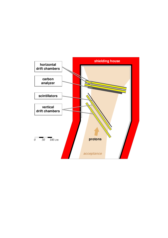
Figure 1: Setup of the proton polarimeter in the shielding house of Spectrometer A. The standard detector system is supplemented by a carbon analyzer and two double-planes of HDCs for proton tracking after scattering.

The shielding house of Spectrometer A is indicated in dark grey. The light-grey shaded band indicates possible proton trajectories. They cross, from bottom to top, the two VDCs and the scintillators, and then impinge on the graphite analyzer. Its thickness can be optimized between 1 and 7 cm (density $\rho=1.76$ g/cm³) for protons up to the spectrometer’s maximum central momentum of 660 MeV/c. With an active area of $2178\times 749.5$ mm² the HDCs are large enough to measure proton scattering angles of up to $20^{\circ}$ over the full size of the carbon analyzer. This covers the region of high analyzing power. Even between $20^{\circ}$ and $35^{\circ}$, $97.7\,\%$ of the scattered protons are geometrically accepted. The HDCs are the crucial new parts of the polarimeter setup. They are described in detail in the next section.

3 Horizontal drift-chambers

The polarimeter HDCs realize a simple geometry which is similar to early designs [31, 32]. The electric field is formed by alternating so-called potential wires and signal wires. In our case the former are grounded whereas the latter carry positive high voltage of typically 3000 V.

All wires of the polarimeter HDCs are gold-plated tungsten with diameters of 50 and 100 $\mu$m for the signal and potential wires, respectively. Each wire plane consists of 103 signal wires and 104 potential wires. Their maximum length is 106 cm because they are stretched under 45^∘ across the wire frames. The wires of the two individual planes of a double-plane are perpendicular to each other.

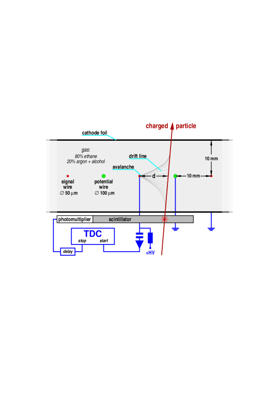
Figure 2: Schematics of the HDC. The field forming signal and potential wires have a distance of 1 cm to each other and to the cathode foils. Electrons from the ionization along the particle track drift to the signal wire. The drift time measurement is started by the individual signal wires and stopped by a fast external trigger scintillator.

As can be seen from the schematical drawing of Figure 2 the wire separation is 10 mm. This is also the distance between the wire plane and the cathode foils, which consist of 6 $\mu$m Mylar with double sided aluminium coating. A single drift cell has a cross section of $20\times 20$ mm².

An incoming charged particle creates electron-ion pairs along its track. With our gas composition of 20 % argon and 80 % ethane protons of 150 MeV kinetic energy have a specific energy loss of $dE/dx=7.6$ keV/cm at normal pressure. This results in approximately 290 electron-ion pairs per cm. The electrons drift to the nearest signal wire, in the vicinity of which the gas amplification occurs. The signals are fed through a high voltage capacitor to standard LeCroy 2735DC amplifiers/discriminators, whose outputs then start time-to-digital converters (TDC) of a TDC2001 system [33] individually for each signal wire. The drift time is measured against the standard trigger-scintillator plane of Spectrometer A which stops the TDC after an appropriate delay.

With known drift velocity of the electrons the TDC information can be converted into drift distance. For the given gas composition the drift velocity, $v_{D}$, depends on the reduced field strength, $E/p$. Both the field strength in the drift cell and the drift velocity are shown in Figure 3.

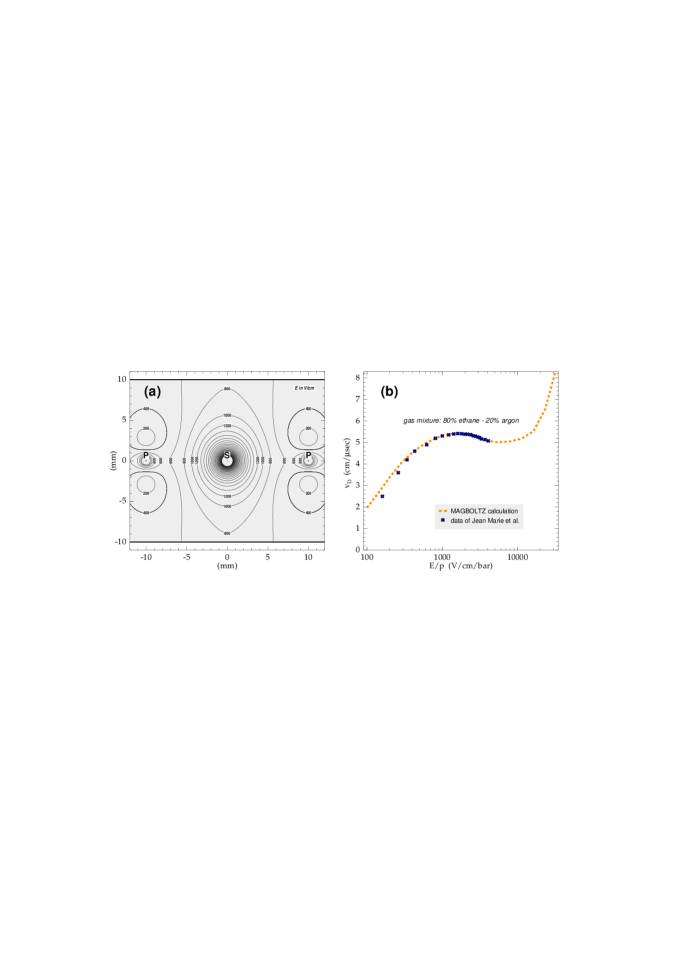
Figure 3: (a) Contour lines of the electric field strength in a drift cell. Cathode foils and potential wires (P) grounded, signal wires (S) on +3000 V. Calculated with the computer code GARFIELD [34]. (b) Electron drift velocity in a gas mixture of 80 % ethane and 20 % argon as a function of pressure-normalized electrical field strength. Calculation (dashed line) with the computer code MAGBOLTZ [35] compared to measurement (crosses) [36].

Except at the ‘corners’ above and below the potential wires the field strength is in the range 0.4 – 15 kV/cm. Thus, at normal pressure the drift velocity has values within $\pm 10$ % around $v_{D}\simeq 5$ cm/$\mu$s; this plateau makes the operation of the HDC insensitive against small changes of the external conditions, e.g. air pressure and high voltage.

At a field strength of 1 kV/cm the longitudinal diffusion broadening is only 100 $\mu$m per cm of drift [36], which is a factor of ten better than in pure argon. Furthermore, with 80 % ethane as photon quencher a gas amplification of $10^{4}$ – $10^{6}$ can be achieved with well localized avalanches, which is 1 – 2 orders of magnitude higher than in pure argon. The localization of the avalanches plays a crucial role for the left-right assignment in the HDC.

3.1 Left-right assignment

A standard problem in HDCs is the left-right ambiguity: From the measurement of a single drift time it cannot be decided whether the particle track occured left or right of the signal wire. However, if the avalanches are well localized on the particle track’s side of the signal wire [37], different signals are induced on the two potential wires bounding a drift cell; the signal is larger on that side of the signal wire where the avalanche occured [38]. The potential wire signals are approximately an order of magnitude below those of the signal wires, and the difference between the potential wire signals is another factor of ten smaller. Assuming a few hundred avalanches of about $5\times 10^{5}$ electron-ion pairs from a particle track, for the given geometry and operating conditions a difference signal of $\Delta I\simeq 100$ nA is obtained over a time-interval of 200 – 300 ns.

In order to exploit the small difference between the potential wire signals a special so-called left-right amplifier has been designed and built [39, 40]. Its circuit diagram is schematically depicted in Figure 4.

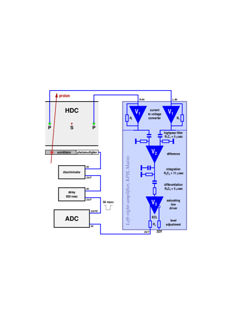
Figure 4: The left-right amplifier’s principle of operation. Signals of adjacent potential wires after linear amplification are fed to a differential amplifier. The output signal is integrated in an ADC.

The currents induced on adjacent potential wires first are converted to a voltage by the amplifiers V₁. The feedback resistors R_f have to be equal within $0.1\,\%$ in order to achieve a common mode rejection of typically 50 dB for the differential amplifier V₂. Due to the low input-impedance of V₁ a ‘sectoring’, i.e. the combination of the potential wires from several cells, is possible: Each wire plane is divided into 10 odd-even sectors of 7 (full-length) up to 20 (shorter - in the corners of the HDC) drift cells in which all odd and even numbered potential wires, respectively, are bussed together into one input of V₁. An additional left-right amplifier is used for each drift cell inbetween two sectors. Therefore the whole plane is read out by 19 ‘odd-even’ amplifiers.

The output signal of the differential amplifier V₂ in Figure 4 is integrated and then differentiated in order to achieve a recovery time of better than 20 $\mu$s after overload. After further amplification and level shifting in V₃, the output pulses are fed to a 96-channel LeCroy 1882N analog-to-digital converter (ADC). There the signal is integrated for 50 ns. The ADC gate is delayed by 650 ns relative to the trigger scintillator.

A typical odd-even spectrum is shown in Figure 5.

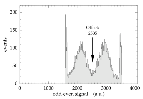
Figure 5: ADC-spectrum for one odd-even sector.

If the current-difference between odd and even wires of a sector $I_{odd}-I_{even}<-90$ nA, then the output of the odd-even amplifier is in negative saturation which shows up as the right peak in the ADC spectrum. For $I_{odd}-I_{even}>90$ nA the amplifier is in positive saturation and the corresponding events are located in the left peak of Figure 5. The amplifier’s output is proportional to the input-current difference when $|I_{odd}-I_{even}|<90$ nA.

Events in the left and right parts correspond to tracks through the ‘even’ and ‘odd’ side of the sector, respectively. Entries around the central minimum of spectrum are mainly due to tracks close to the signal wire. The good performance of the left-right decision was confirmed through measurements without carbon analyzer, both with the large HDCs and with a small prototype HDC [41].

3.2 Drift time and drift distance

After the correct left-right assignment the drift time can be interpreted in terms of a position coordinate perpendicular to the actual wire direction. Despite the plateau in the drift-velocity distribution of Figure 3 the assumption of a constant drift velocity is too rough an approximation. If the drift cell is uniformly illuminated, a detailed relation between drift time and drift distance can be established from the drift-time spectrum (cf. Figure 6 top left) itself.

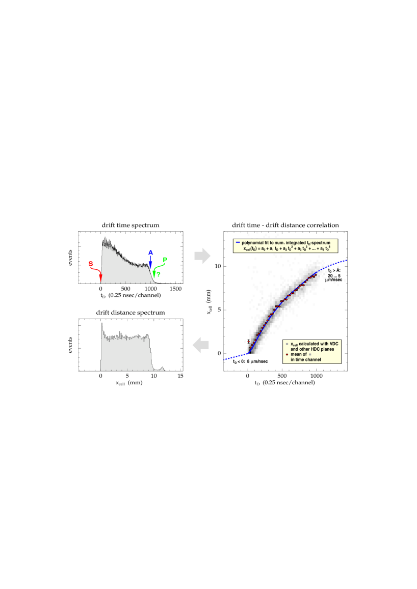
Figure 6: Drift-time (top left) and drift-distance (bottom left) spectra and relation between time and distance (right) as obtained by numerical integration of the time spectrum. For explanation see text.

The drift times cover a range of 0 – 250 ns which corresponds to the wire spacing of 1 cm and the average drift velocity of almost 5 cm/$\mu$s. The non-flatness of this spectrum reflects the differential deviations of the drift velocity from the mean value.

Each drift-time interval $[t_{D},t_{D}+\Delta t_{D}]$ can be attached to a drift-distance interval $[x_{cell},x_{cell}+\Delta x_{cell}]$. The number of events in this time interval, $\Delta N(t_{D})$, is given by the number of events in the correponding drift-distance interval, $\Delta N(x_{cell})$, and the time interval is related to the drift-distance interval through the local drift velocity, $v_{D}(x_{cell})$:

$$\frac{\Delta N(t_{D})}{\Delta t_{D}}=\frac{\Delta N(x_{cell})}{\Delta x_{cell}/v_{D}(x_{cell})}=\frac{\Delta N(x_{cell})}{\Delta x_{cell}}\cdot\frac{\Delta x_{cell}(t_{D})}{\Delta t_{D}}.$$ (2)

Uniform illumination of the drift cells yields constant $\Delta N(x_{cell})/\Delta x_{cell}$. Therefore the relation between $x_{cell}$ and $t_{D}$ can be determined by integration of the drift-time spectrum:

$$x_{cell}(t_{D})=x_{cell}(A)\cdot\frac{\int_{0}^{t_{D}}\frac{dN(t)}{dt}dt}{\int_{0}^{t_{D}(A)}\frac{dN(t)}{dt}dt}.$$ (3)

The lower limit of integration, $t_{D}=0$, is related to tracks directly at the signal wire (indicated by S in the drift-time spectrum of Figure 6). However, the upper limit, $t_{D}(A)$, is not very well determined due to the decrease of efficiency in the regions of reduced field strength close to the potential wires (compare Figure 3a). Therefore the ‘position’ of the potential wire in the drift-time spectrum (indicated by P) is not well defined. Instead, as the upper integration limit in Eq. 3 the edge indicated by A is used which corresponds to the decline of the efficiency.

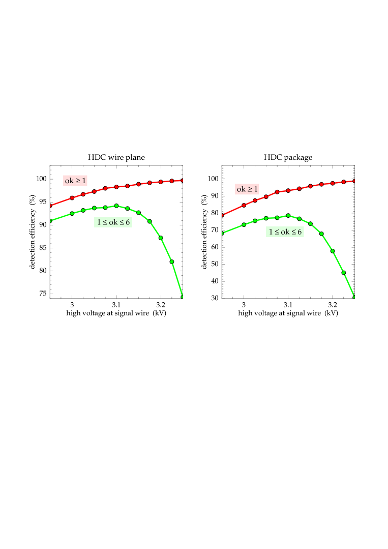
Figure 7: HDC efficiency as a function of high voltage for protons of $T_{HDC}=130$ MeV kinetic energy and a rate of $2.5$ kHz at the HDC, and a discriminator threshold adjusted to $U_{thres.}=7$ V at the LeCroy 2735DC amplifier/discriminator (corresponding to a current threshold of 14 $\mu$A). The left part is for one single plane, the projection to the total efficiency of the 4-plane package is shown right. The $ok$ classification is described in the text.

The drift-time to drift-distance relation is fitted by an 8^th order polynomial, which is shown as full curve in the right part of Figure 6. It is confirmed by extrapolating particle trajectories measured with the VDCs to the bottom plane of the HDC-package of the polarimeter. These extrapolation results are indicated grey in the right plot, and the column-wise mean values are represented by the points. For standard operating conditions best agreement between measurement and the numerical integration in Eq. 3 is obtained with $x_{cell}(A)=9.3$ mm. The continuation of the polynomial over the bounding of the drift cell in order to get a continuous relation is somewhat arbitrary.

From the drift-time to drift-distance relation the drift-distance spectrum (bottom left in Figure 6) is obtained. Events at $x_{cell}>11$ mm are due to very long drift times $t_{D}>400$ ns. They are attributed to tracks through the edges of the drift cells where the field strength is low. The peak at small distances between 200 and 500 $\mu$m is due to the fact that for particle tracks with zero distance to the signal wire a sufficient number of avalanches does not occur before a short delay. This effect does not produce errors larger than the position resolution of the HDCs, which was determined to $\delta x\simeq 300$ $\mu$m from measurements of proton tracks with the prototype HDC relative to the standard VDCs. With the distance of 22 cm between the two HDC double-planes an angular resolution of approximately 2 mrad is achieved.

3.3 HDC efficiency

The efficiency of three of the four HDC planes can be measured by a ‘sandwich’ method: If both the standard VDCs and the top HDC fired, then the particle also must have crossed the lower HDC planes. The result for the efficiency for one of these planes is shown in the left part of Figure 7, the projection to the total efficiency of the 4-plane HDC package in the right part.

HDC events are classified according to their hit pattern. In the data analysis so-called $ok$ numbers are established. Single hits and adjacent double hits get $1\leq ok\leq 6$, whereas $ok>6$ is related to the occurence of non-adjacent double or multiple hits, electronic crosstalk, negative drift times, etc, which go along with an increased error probability for the calculated trajectory. The efficiency rises monotonically with the applied voltage if events with any hit pattern ($ok\geq 1$) are taken into account. This, however, is not the case for the useful events with $1\leq ok\leq 6$, where the efficiency shows a clear maximum around $3.1$ kV. This is due to the fact that multiple hits and crosstalk are much enhanced above the optimum high voltage. The results depicted in Figure 7 depend on the particle ionization density and on the threshold of the amplifier/discriminator. Furthermore, the efficiency depends on the orientation of the particle trajectory relative to the HDC planes. This will be reconsidered as a source of false systematic asymmetries in the polarization measurements.

4 Measurement of proton polarization

The detector setup in Spectrometer A (compare Figure 1) enables a measurement of the proton trajectories before and after scattering in the carbon analyzer. Therefore the polar and azimuthal scattering angles can be determined as required for the polarization analysis. It is also possible to extract the position of the scattering vertex. This is necessary for a separation of events scattered in the carbon analyzer from those scattered e.g. in the scintillator planes of the spectrometer. Furthermore, a diagnosis of errors both in the VDCs and in the HDCs becomes possible [19].

Figure 8 shows the distribution of the polar scattering angle $\Theta_{s}$ measured with a 7 cm thick carbon analyzer. The proton kinetic energies varied between 170 and 260 MeV across the acceptance of the spectrometer. In contrast to other focal-plane polarimeters no small-angle rejection [42] was used. Therefore the spectrum is dominated by small scattering angles $\Theta_{s}<7^{\circ}$.

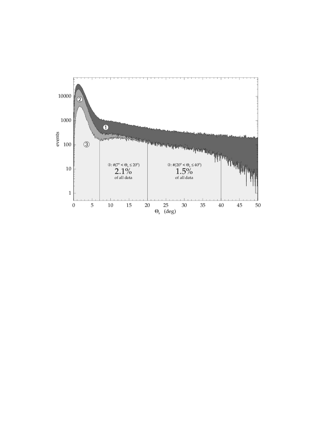
Figure 8: Proton-carbon scattering angles for an analyzer thickness of 7 cm and a proton energy range of 170 – 260 MeV. Curve 1 represents all data whereas in curve 2 events with drift chamber errors are discarded. In spectrum 3 a scattering vertex within the carbon analyzer is required, which also suppresses events with small scattering angles.

The efficiency of the polarimeter is related to the small fraction of $2.1$ % of events in the angular range $7^{\circ}<\Theta_{s}\leq 20^{\circ}$, where the analyzing power is large and well known [28, 29]. The analyzing power at larger angles is reconsidered in subsection 4.2.1.

The proton polarization is determined according to Eq. 1 from the azimuthal angular distribution. Such distributions are shown in Figure 9 from the $p(\vec{e},e^{\prime}\vec{p}\,)$ elastic scattering reaction for two cases labelled ‘helicity-sum’ (a) and ‘helicity-difference’ (b).

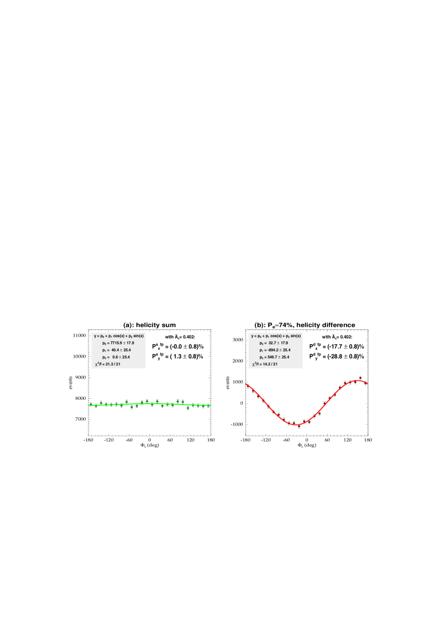
Figure 9: Azimuthal angular distribution measured in the proton polarimeter for $p(\vec{e},e^{\prime}\vec{p}\,)$ elastic scattering. As explained in the text, the ‘helicity-sum’ spectrum (a) is expected to be flat, whereas the ‘helicity-difference’ (b) shows an asymmetry proportional to the recoil polarization. In this example the beam polarization was $P_{e}\simeq 74$ %.

In elastic electron-proton scattering the recoil proton polarization is proportional to the longitudinal polarization of the electron beam [43, 44] and thus flips sign under reversal of beam-helicity. During the experiment the electron-beam helicity is flipped at the source [45] on a random basis with a frequency of 1 Hz. Therefore the sum of events with positive and negative helicity corresponds to unpolarized beam and no azimuthal modulation must occur in Figure 9(a). In contrast, in the difference of the $\Phi$-distributions for positive and negative beam helicities (Figure 9(b)) the asymmetries add up. In the ‘helicity-difference’ distribution instrumental asymmetries – which of course are independent of beam helicity – cancel out. This is not the case for the ‘helicity-sum’. Although there are no large instrumental effects visible in Figure 9(a) the false systematic asymmetries are analyzed in more detail in section 4.2.2. Eventwise calculation of the analyzing power according to the parameterization [29] yielded for the data of Figure 9 a mean value of $\bar{A}_{C}=0.402$.

In general, from the ‘helicity-sum’ distribution it is possible to extract two beam-helicity independent recoil polarization components, while from the ‘helicity-difference’ two beam-helicity dependent components are obtained. However, these polarizations are measured behind the spectrometer’s focal plane, i.e. after spin precession in a magnetic system. In order to determine the proton polarization at the electron scattering vertex relative to the frame of the electron scattering plane, which is defined through the incident and scattered electron momenta $\vec{p}_{i}$ and $\vec{p}_{f}$, respectively,

$$\hat{z}=\frac{\vec{p}_{i}-\vec{p}_{f}}{|\vec{p}_{i}-\vec{p}_{f}|},\quad\hat{x}=\frac{\vec{p}_{i}\times\vec{p}_{f}}{\vec{p}_{i}\times\vec{p}_{f}},\quad\hat{y}=\hat{z}\times\hat{x},$$ (4)

the polarization measured in the focal plane must be traced back through the fields of the spectrometer. Despite the obvious complication, it is only through the spin precession that the longitudinal polarization component (in the direction of the proton momentum at the electron vertex) becomes accessible.

4.1 Spin precession

The description of the precession of a spin vector $\vec{S}$ in Spectrometer A is based on the Thomas equation [46]. For pure magnetic fields it can be cast into the form

$$\frac{d\vec{S}}{dt}=\frac{e}{m\gamma}\vec{S}\times\left[\frac{g}{2}\vec{B}_{\parallel}+(1+\frac{g-2}{2}\gamma)\vec{B}_{\perp}\right],$$ (5)

where $e$ and $m$ are the particle’s charge and mass, and $g$ is its $g$-factor; $\gamma$ is the Lorentz-factor and the magnetic field is split into two parts, $\vec{B}_{\parallel}$ and $\vec{B}_{\perp}$, which are parallel and perpendicular to the particle’s momentum, respectively.

In its vertical midplane the QSDD-type Spectrometer A [22] can be approximated as a pure dipole with no longitudinal fields. In this case for a Dirac particle with $g=2$ the precession of the spin-vector is the same as for the momentum vector. However, due to the large anomalous magnetic moment of the proton ($g=5.586$) its spin precesses against its direction. For a momentum of $p_{p}=630$ MeV/c the spin precession angles vary between $191^{\circ}$ and $242^{\circ}$ across the dispersive (i.e. the vertical) acceptance of the spectrometer. It is important to have the spin precession around $45^{\circ}$ (modulo $90^{\circ}$) in order to achieve enough sensitivity to the polarization components both in longitudinal and in dispersive direction at the electron vertex.

In general, the spin precession through the spectrometer is complicated due to the longitudinal fields and the varying bending directions in the consecutive optical elements. It is computed with the C++ code QSPIN [19] which evolves both momentum and spin along the trajectories using a Runge-Kutta method with adaptive stepsize according to Cash and Karp [47, 48]. QSPIN calculates the required magnetic field components similar to the RAYTRACE code [49], which originally was used for the design of the spectrometer’s optics. The QSPIN results for protons of $p_{p}=630$ MeV/c with spins oriented in $\hat{z}$ direction at the target are visualized in Figure 10 for three trajectories with different so-called spectrometer-target coordinates $\Theta_{0}^{tg}$ (dispersive angle), $y_{0}^{tg}$ (long target coordinate) and $\Phi_{0}^{tg}$ (non-dispersive angle). Obviously, the different trajectories result in completely different spin orientations behind the magnetic system.

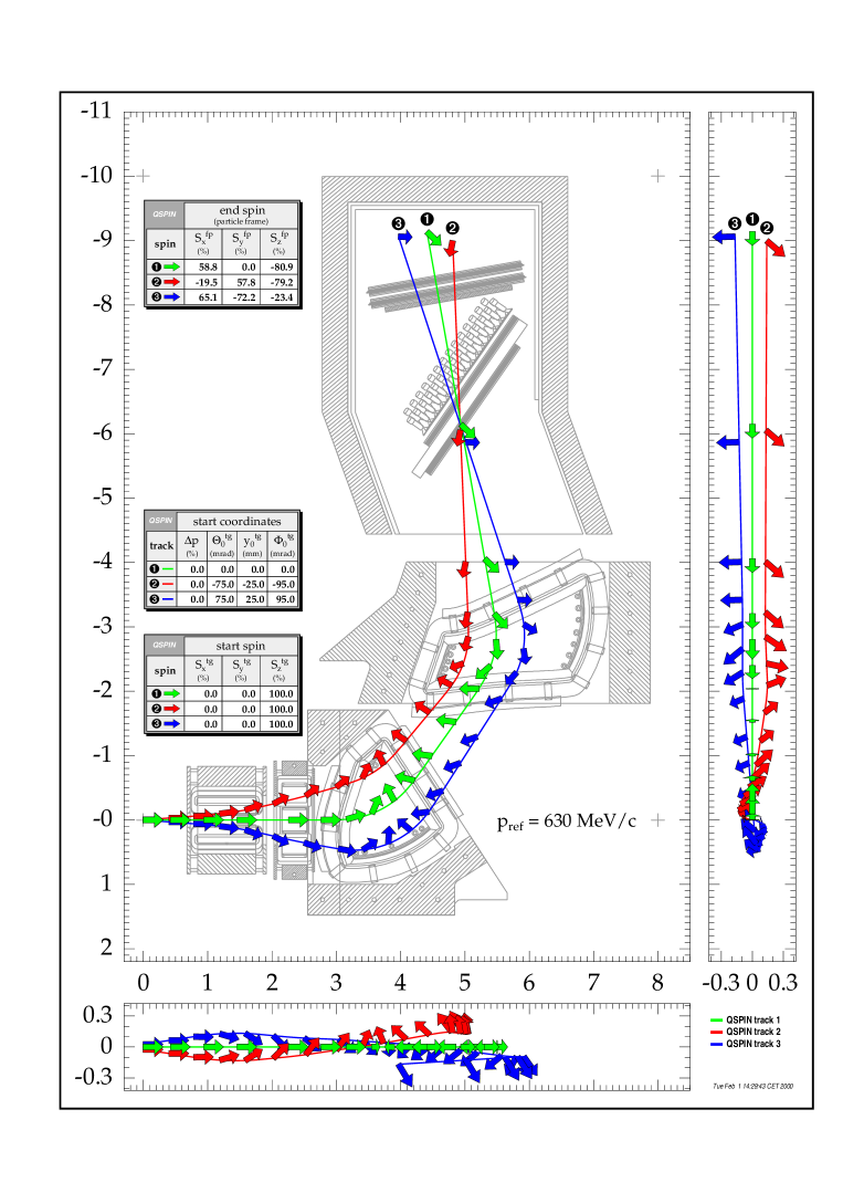
Figure 10: Side view of the spin precession in Spectrometer A, calculated with QSPIN for three proton trajectories. Different spectrometer-target coordinates result in a completely different precession of the spins, which initially were oriented in the same direction. Also shown are the rear and bottom projections of the proton tracks and spins. The scale is in meters.

Since the spin precession is a rotation of the initial spin in the spectrometer-target frame (tg) into the final direction in the particle frame behind the focal plane (fp, c.f. Figure 10), it can be written in matrix form:

$$\left(\begin{array}[]{c}S_{x}\\ S_{y}\\ S_{z}\\ \end{array}\right)^{fp}=\left(\begin{array}[]{ccc}M_{xx}&M_{xy}&M_{xz}\\ M_{yx}&M_{yy}&M_{yz}\\ M_{zx}&M_{zy}&M_{zz}\\ \end{array}\right)\left(\begin{array}[]{c}S_{x}\\ S_{y}\\ S_{z}\\ \end{array}\right)^{tg}\,.$$ (6)

Similar to the case of its optics matrix, the elements of the spectrometer’s spin transfer matrix (STM), $M_{\kappa\lambda}$, can be expressed as polynomials in the spectrometer-target coordinates $\Theta_{0}^{tg}$, $y_{0}^{tg}$, $\Phi_{0}^{tg}$, the reference momentum setting $p_{ref}$ of the spectrometer and the deviation $\Delta p$ of the particle’s momentum from $p_{ref}$:

$$M_{\kappa\lambda}=\sum_{ijklm}\langle M_{\kappa\lambda}|\Delta p^{i}\,\Theta_{0}^{j}\,y_{0}^{k}\,\Phi_{0}^{l}p_{ref}^{m}\rangle\,\Delta p^{i}\,\Theta_{0}^{j}\,y_{0}^{k}\,\Phi_{0}^{l}\,p_{ref}^{m}$$ (7)

with $i,j,k,l,m\in N$ and $\kappa,\lambda\in{x,y,z}$. The polynomial coefficients were determined by $\chi^{2}$ minimization of pseudo data. Those were generated by QSPIN on 1715 different trajectories across the spectrometer’s acceptance for each of three initial spin orientations at the target and six different momentum settings within $p_{ref}=480$–$630$ MeV/c (which covers the momentum range in which the polarimeter can be operated).

In a real experiment the polarization is measured behind the magnetic deflection and must then be traced back through the spectrometer. However, the STM cannot be inverted directly, because only two polarization components are measurable in the polarimeter. Nevertheless, there is a twofold redundancy that can be exploited:

1. The electron-helicity dependent and independent parts of the recoil polarization can be separated by differences and sums of the measured asymmetries, respectively (compare beginning of section 4). Symmetric averaging around the direction of momentum transfer yields for certain reactions (see for example [14]) the two recoil polarization components in the electron scattering plane (longitudinal and transversal), which are beam-helicity dependent, and the normal component, which is helicity independent.

2. Events from the same physical situation (and thus with the same recoil polarization) are obtained with different spectrometer-target coordinates due to, e.g., the possible tilting of the electron scattering plane against Spectrometer A or the distribution of scattering vertices over the target length. The related large variation of the spin precession is exploited in the following fitting procedure.

The two focal plane polarization components are related to the polarization at the scattering vertex (in the frame of Eq. 4) by

$$\left(\begin{array}[]{c}P_{x}\\ P_{y}\\ \end{array}\right)^{fp}=\left(\begin{array}[]{ccc}M_{xx}&M_{xy}&M_{xz}\\ M_{yx}&M_{yy}&M_{yz}\\ \end{array}\right)\cdot T_{\lambda\xi}\cdot\left(\begin{array}[]{c}P_{x}\\ P_{y}\\ P_{z}\\ \end{array}\right)^{sp},$$ (8)

or

$$P_{\kappa}^{fp}=\sum\limits_{\lambda=x}^{z}\sum\limits_{\xi=x}^{z}M_{\kappa\lambda}(\Delta p,\Theta_{0}^{tg},y_{0}^{tg},\Phi_{0}^{tg},p_{ref})\;T_{\lambda\xi}(\Theta^{h}_{e},\Phi^{h}_{e},|\vec{p}_{f}|,|\vec{p}_{i}|,\Phi_{A})\;P_{\xi}^{sp}\;,$$ (9)

with $\kappa=x,y$. $T_{\lambda\xi}\,=\,\hat{\lambda}^{tg}\cdot\hat{\xi}^{sp}$ with $\lambda,\xi\in\{x,y,z\}$ is the $3\times 3$ matrix describing the rotation between the coordinate frames of spectrometer-target and scattering plane. The angles $\Theta^{h}_{e}$ and $\Phi^{h}_{e}$ characterize the direction of the scattered electron and $\Phi_{A}$ is the central angle of Spectrometer A relative to the incident beam. The matrix product yields the complete $3\times 2$ imaging matrix $F_{\kappa\xi}(\vec{x})=\sum\limits_{\lambda=x}^{z}M_{\kappa\lambda}\cdot T_{\lambda\xi}$ with $\vec{x}=(\Delta p,\Theta_{0}^{tg},y_{0}^{tg},\Phi_{0}^{tg},p_{ref},\Theta^{h}_{e},\Phi^{h}_{e},|\vec{p}_{f}|,|\vec{p}_{i}|,\Phi_{A})$.

In order to enable fitting, the acceptance in $\vec{x}$ is subdivided into $N_{D}$ bins for which the focal plane polarization is measured separately as $P^{fp}_{x,i}(\vec{x_{i}})$ and $P^{fp}_{y,i}(\vec{x_{i}})$ with errors $\Delta P^{fp}_{x,i}(\vec{x_{i}})$ and $\Delta P^{fp}_{y,i}(\vec{x_{i}})$, $i=1,...,N_{D}$. Under the assumption that the components $P_{x,y,z}^{sp}$ themselves are independent of $\vec{x}$ they can be determined by minimizing

$$\chi^{2}=\sum\limits_{i=1}^{N_{D}}\left(\left[\frac{P^{fp}_{x,i}(\vec{x_{i}})-\sum\limits_{\xi=x}^{z}F_{x\xi}(\vec{x}_{i})P_{\xi}^{sp}}{\Delta P^{fp}_{x,i}(\vec{x_{i}})}\right]^{2}+\left[\frac{P^{fp}_{y,i}(\vec{x_{i}})-\sum\limits_{\xi=x}^{z}F_{y\xi}(\vec{x}_{i}))P_{\xi}^{sp}}{\Delta P^{fp}_{y,i}(\vec{x_{i}})}\right]^{2}\right)\,.$$ (10)

The requirements $\frac{\partial\chi^{2}}{\partial P_{\xi}^{sp}}=0$ lead to the matrix equation

$$A\cdot\vec{P}^{sp}=\vec{b},$$ (11)

where the elements of the $3\times 3$ matrix $A$ and of the vector $\vec{b}$ are given by

$$A_{\xi\mu}=\sum\limits_{i=1}^{N_{D}}\left(\frac{F_{x\xi}(\vec{x}_{i})F_{x\mu}(\vec{x}_{i})}{(\Delta P^{fp}_{x,i}(\vec{x_{i}}))^{2}}+\frac{F_{y\xi}(\vec{x}_{i})F_{y\mu}(\vec{x}_{i})}{(\Delta P^{fp}_{y,i}(\vec{x_{i}}))^{2}}\right),$$ (12)

$$b_{\mu}=\sum\limits_{i=1}^{N_{D}}\left(\frac{P^{fp}_{x,i}(\vec{x_{i}})F_{x\mu}(\vec{x}_{i})}{(\Delta P^{fp}_{x,i}(\vec{x_{i}}))^{2}}+\frac{P^{fp}_{y,i}(\vec{x_{i}})F_{y\mu}(\vec{x}_{i})}{(\Delta P^{fp}_{y,i}(\vec{x_{i}}))^{2}}\right)\;.$$ (13)

The polarization is finally found as

$$\vec{P}^{sp}=A^{-1}\cdot\vec{b}$$ (14)

with the (correlated) error

$$\Delta P^{sp}_{\xi}=\sqrt{(A^{-1})_{\xi\xi}}.$$ (15)

4.2 Elastic $p(\vec{e},e^{\prime}\vec{p}\,)$ measurements

The calculation of the spin precession with QSPIN and the trace back of the polarization measured in the focal plane polarimeter to the electron vertex was checked with elastic $p(\vec{e},e^{\prime}\vec{p}\,)$ measurements. For a given degree of longitudinal electron polarization $P_{e}$, the recoil proton polarization is determined [43, 44] by electron kinematics and by the proton’s Sachs form factors $G_{E}$ and $G_{M}$, which, at low $Q^{2}$, are known at the one-percent level:

$$P_{x}^{sp} = P_{e}\frac{aG_{E}G_{M}}{G_{E}^{2}+cG_{M}^{2}},$$ (16)

$$P_{y}^{sp} = 0,$$ (17)

$$P_{z}^{sp} = P_{e}\frac{bG_{M}^{2}}{G_{E}^{2}+cG_{M}^{2}}.$$ (18)

The axes are defined according to Eq. 4 and the kinematical factors

$$a = -2\sqrt{\tau(1+\tau)}\tan\frac{\theta_{e}}{2},$$ (19)

$$b = -a\sqrt{\tau(1+\tau\sin^{2}\frac{\theta_{e}}{2})}/\cos\frac{\theta_{e}}{2}\qquad\mbox{and}$$ (20)

$$c = \tau+\frac{1}{2}a^{2}$$ (21)

are fixed by the electron scattering angle, $\theta_{e}$, and the squared four-momentum transfer in units of the proton rest mass, $\tau=Q^{2}/4m_{p}^{2}$.

Figure 11: The two transverse polarization components after the spin precession in the spectrometer as a function of the measured dispersive angle (left), the target-length coordinate (middle) and the non-dispersive angle (right). The curves represent the QSPIN calculations described in the text and the data points are the results of the elastic $p(\vec{e},e^{\prime}\vec{p}\,)$ measurements.

For the two transverse polarization components in the focal plane, $P_{x}^{fp}$ and $P_{y}^{fp}$, Figure 11 shows the comparison between QSPIN calculation (curves) and measurement (dots). They agree very well as a function of the spectrometer-target coordinates $\Theta_{0}^{tg}$, $y_{0}^{tg}$ and $\Phi_{0}^{tg}$.

From the polarization components in the scattering plane, $P_{x}^{sp}$ and $P_{z}^{sp}$, it is possible, as can be seen from Eqs. 16 and 18, to determine the beam polarization independently of the proton form factors:

$$P_{e}=\frac{b}{a^{2}}\frac{(P_{x}^{sp})^{2}}{P_{z}^{sp}}+\frac{c}{b}P_{z}^{sp}.$$ (22)

The beam polarizations extracted from the measured proton polarization components were confirmed within a relative error of $2.5$ % [50] by the new Møller polarimeter of the A1 collaboration at MAMI [51]. This also confirms the absolute height of the proton-carbon analyzing power.

4.2.1 Analyzing power at large scattering angles

While in the relevant energy range below 250 MeV the inclusive proton-carbon analyzing power is known at the 2 % level for scattering angles up to 20^∘, the accuracy is much lower for larger angles [28, 29, 52]. However, as can be seen from Figure 8, almost half of the large-angle scattering events are in the range 20^∘ – 50^∘ due to the large angular acceptance of the HDCs. These data were used to determine the analyzing power for large scattering angles relative to the lower angular range. The results are summarized in Table 1 and in Figure 12 for three proton kinetic energies in the center of the carbon analyzer, $T_{CC}$. The acceptance in $T_{CC}$ is approximately $\pm 10$ MeV around the mean values.

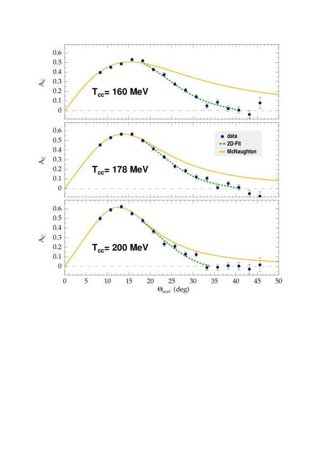
Figure 12: Data of Table 1 (full circles) in comparison with the McNaughton parametrization [29] (full curve). The broken curve represents the fit (Eq. 23) to the data points.

	$T_{\rm CC}$ = 160 MeV	$T_{\rm CC}$ = 178 MeV	$T_{\rm CC}$ = 200 MeV
$\Theta_{\rm s}$	$A_{\rm C}$	$A_{\rm C}$	$A_{\rm C}$
8.3∘	0.396$~{}\pm$  0.013	0.454  $\pm$  0.013	0.500  $\pm$  0.018
10.7∘	0.451$~{}\pm$  0.012	0.530  $\pm$  0.013	0.589  $\pm$  0.017
13.2∘	0.486$~{}\pm$  0.012	0.566  $\pm$  0.014	0.623  $\pm$  0.018
15.7∘	0.531$~{}\pm$  0.013	0.566  $\pm$  0.015	0.550  $\pm$  0.020
18.2∘	0.518$~{}\pm$  0.015	0.499  $\pm$  0.016	0.478  $\pm$  0.022
20.7∘	0.427$~{}\pm$  0.016	0.414  $\pm$  0.017	0.366  $\pm$  0.022
23.2∘	0.374$~{}\pm$  0.017	0.328  $\pm$  0.018	0.234  $\pm$  0.023
25.7∘	0.276$~{}\pm$  0.018	0.231  $\pm$  0.019	0.210  $\pm$  0.023
28.2∘	0.212$~{}\pm$  0.019	0.186  $\pm$  0.020	0.128  $\pm$  0.024
30.7∘	0.145$~{}\pm$  0.021	0.120  $\pm$  0.020	0.124  $\pm$  0.025
33.2∘	0.048$~{}\pm$  0.022	0.106  $\pm$  0.021	-0.011  $\pm$  0.027
35.7∘	0.087$~{}\pm$  0.024	0.010  $\pm$  0.023	-0.008  $\pm$  0.030
38.2∘	0.021$~{}\pm$  0.028	0.052  $\pm$  0.025	0.008  $\pm$  0.034
40.7∘	0.004$~{}\pm$  0.033	0.012  $\pm$  0.029	0.004  $\pm$  0.040
43.1∘	-0.041$~{}\pm$  0.042	-0.053  $\pm$  0.036	-0.027  $\pm$  0.050
45.6∘	0.080$~{}\pm$  0.056	-0.081  $\pm$  0.050	0.017  $\pm$  0.070

Table 1: Inclusive p - ¹²C analyzing power as a function of scattering angle $\Theta_{s}$, measured with polarized protons from the elastic $p(\vec{e},e^{\prime}\vec{p}\,)$ reaction.

Figure 12 shows that these data agree well with the McNaughton parameterization [29] up to scattering angles of 20 degrees, the limit of its validity. They are also in agreement with earlier large angle data [52] with larger errors. The result of the $\chi^{2}$ minimization of the two-dimensional polynomial

$$A_{C}(\Theta_{s},A_{CC})=\sum_{i=0}^{2}\sum_{j=0}^{4}a_{ij}(T_{CC}/\mbox{MeV})^{i}(\Theta_{s}/\mbox{deg})^{j}$$ (23)

for the data between $\Theta_{s}=15.7$ and $43.1$ degrees is shown as broken line in Figure 12, and the parameters $a_{ij}$ are given in Table 2.

$a_{ij}$	$j=0$	$j=1$	$j=2$	$j=3$	$j=4$
$i=0$	-18.5902	1.47447	-0.0184451	-0.00084808	1.66656e-05
$i=1$	0.162901	-0.00897434	-0.000186479	1.81209e-05	-2.56371e-07
$i=2$	-0.00034948	1.18913e-05	1.10527e-06	-6.23088e-08	8.07095e-10

Table 2: Coefficients of the polynomial Eq. 23 in the range $\Theta_{s}=15.7^{\circ}-43.1^{\circ}$ and $T_{CC}=160-200$ MeV

4.2.2 False asymmetries

In order to avoid false asymmetries at the edges of the acceptance, each event with scattering angles $\Theta_{s}$ and $\Phi_{s}$ is only accepted, if in opposite azimuthal direction, $\Phi_{s}+\pi$, it would have been accepted, too. This geometrical acceptance test does, however, not avoid artificial asymmetries which are due to systematic efficiency variations. As was mentioned in section 3.3 the detection efficiency of the HDCs depends on the orientation of the proton tracks relative to the HDC planes. This potentially produces false asymmetries. In contrast to the beam-helicity dependent polarization components which are extracted from the ‘helicity-difference’ (compare Figure 9), the ‘helicity-sum’ is fully sensitive to such effects.

According to Eq. 17 the beam-helicity independent recoil polarization must vanish in the elastic $p(\vec{e},e^{\prime}\vec{p}\,)$ reaction. Therefore any measured ‘helicity-sum’ asymmetry is false. In Figure 13 the false asymmetries $A_{x}^{f}$ and $A_{y}^{f}$ are plotted as a function of the angles $\Theta_{VTH}$ and $\Phi_{VTH}$ which characterize the orientation of the incoming proton trajectory at the carbon analyzer. The magnitude of the false asymmetries varies with the proton-carbon scattering angle $\Theta_{s}$. It is described by two-dimensional linear fits, the parameters of which are given as inserts in Figure 13. $A_{x}^{f}(\Phi_{VTH},\Theta_{s})$ and $A_{y}^{f}(\Theta_{VTH},\Theta_{s})$ are used to correct $P_{x}^{fp}$ and $P_{y}^{fp}$, respectively.

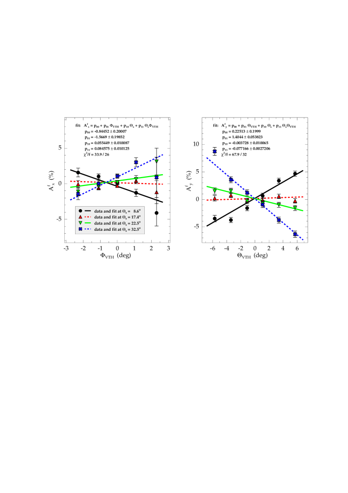
Figure 13: False asymmetries $A_{x}^{f}$ and $A_{y}^{f}$ as a function of the orientation of the incoming proton tracks at the carbon analyzer, characterized through the angles $\Theta_{VTH}$ and $\Phi_{VTH}$. The straight lines represent linear fits. Different symbols and lines are used for scattering angles around $\Theta_{s}=8.6^{\circ},17.4^{\circ},22.5^{\circ}$ and $32.5^{\circ}$ (fits include in addition data at $\Theta_{s}=12.4^{\circ}$ and $27.5^{\circ}$).

4.2.3 Systematic errors

The false asymmetries discussed in the previous subsection only play a role in the beam-helicity independent polarization components. After correction, their remaining absolute contribution to the corresponding polarization components is less than 1 %. The error in the analyzing power contributes with $\pm 2$ % relative.

A major part of the systematic uncertainty comes from the trace back of the polarization through the spectrometer. The quality of the STM and the consistency of the method are confirmed within approximately 1 % through the elastic measurements and through the agreement of the extracted electron-beam polarization with the Møller measurements [50]. In addition, the spin-precession calculation, and thus the trace back, is affected by errors in the spectrometer-target coordinates as determined by Spectrometer A.

Finally, if the recoil polarization is transformed into the electron scattering plane, then also errors from the electron arm contribute. For the elastic $p(\vec{e},e^{\prime}\vec{p}\,)$ reaction, Table 3 gives a compilation of all systematic error contributions for the (helicity-dependent) polarization components in the electron scattering plane as well as for the extracted beam polarization.

		$P^{sp}_{x}$ (%)	$P^{sp}_{z}$ (%)	$P_{e}$ (%)
measured value		-28.5	28.3	73.0
individual syst. errors		$\sigma^{sys}_{P^{sp}_{x}}$	$\sigma^{sys}_{P^{sp}_{z}}$	$\sigma^{sys}_{P_{e}}$
$\Delta\Delta p$ =	$\pm$ 0.2 %	<$\pm$ 0.01	$\mp$ 0.02	<$\pm$ 0.01
$\Delta\Theta_{0}^{tg}$ =	$\pm$ 2 mrad	<$\pm$ 0.01	$\mp$ 0.46	$\mp$ 0.16
$\Delta y_{0}^{tg}$ =	$\pm$ 1.5 mm	$\mp$ 0.40	$\mp$ 0.80	$\pm$ 0.65
$\Delta\Phi_{0}^{tg}$ =	$\pm$ 2 mrad	$\mp$ 0.24	$\mp$ 0.18	$\pm$ 0.54
$\Delta p_{ref}$ =	$\pm$ 0.5 MeV/c	<$\pm$ 0.01	$\mp$ 0.02	$\mp$ 0.01
$\Delta\Theta_{e}^{h}$ =	$\pm$ 2 mrad	<$\pm$ 0.01	$\mp$ 0.12	$\mp$ 0.03
$\Delta\Phi_{e}^{h}$ =	$\pm$ 2 mrad	$\pm$ 0.01	$\mp$ 0.01	$\pm$ 0.05
$\Delta|\vec{p}_{e^{\prime}}|$ =	$\pm$ 0.2 MeV/c	$\pm$ 0.01	$\pm$ 0.01	$\mp$ 0.02
$\Delta|\vec{p}_{e}|$ =	$\pm$ 0.2 MeV/c	$\mp$ 0.01	$\mp$ 0.01	$\pm$ 0.01
$\Delta\Phi_{\rm A}$ =	$\mp$ 1 mrad	$\mp$ 0.03	$\pm$ 0.03	$\pm$ 0.06
$\Delta A_{\rm C}$ =	$\pm$ 2 % (rel.)	$\pm$ 0.57	$\pm$ 0.56	$\pm$ 1.46
total syst. error		$\pm$ 0.74	$\pm$ 1.10	$\pm$ 1.70
statistical error		$\pm$ 0.43	$\pm$ 0.67	$\pm$ 1.02

Table 3: Compilation of systematic errors for the elastic $p(\vec{e},e^{\prime}\vec{p}\,)$ measurement with $T_{CC}=160$ MeV.

In $P_{x}^{sp}$ and $P_{z}^{sp}$ the error is dominated by that of the long-target coordinate $\Delta y_{0}^{tg}$ and to a lesser extent by the errors in the dispersive and non-dispersive angles $\Delta\Theta_{0}^{tg}$ and $\Delta\Phi_{0}^{tg}$, respectively. Also important is the uncertainty $\Delta A_{C}$ of the analyzing power, which dominates the error of the extracted beam polarization $P_{e}$.

5 Summary

Interesting nucleon and nuclear structure effects have recently become accessible in double-polarization, exclusive electron scattering experiments. These experiments require in addition to the longitudinally polarized electron beam either a polarized target or recoil polarimetry. For $(\vec{e},e^{\prime}\vec{p}\,)$-type coincidence experiments a focal plane polarimeter has been added to Spectrometer A of the 3-spectrometer setup of the A1 collaboration at MAMI. The proton polarization is measured through inclusive proton-carbon scattering. To this end, the standard VDC detector system has been supplemented by a graphite analyzer of variable thickness and two double planes of horizontal drift chambers to determine the trajectory of the scattered protons against the incoming proton tracks, which are measured in the VDCs.

The HDCs cover proton-carbon scattering angles up to 45^∘ over the whole area of the analyzer. They are operated with a gas mixture of 20 % argon and 80 % ethane. Integration of the drift-time distribution for a homogeneously illuminated HDC yields the drift-time to drift-distance relation. The left-right ambiguity of the HDC is resolved through readout of the charge signals induced on adjacent potential wires by the ion drift from an avalanche. A position resolution of 300 $\mu$m is achieved corresponding to an angular resolution of 2 mrad.

The measured polarization must be traced back through the magnetic fields of the spectrometer. All three polarization components at the target can be determined simultaneously due to the variation of the spin precession across the acceptance of the spectrometer and the redundancy provided by flipping the electron-beam helicity. The calculation of the precession was checked through the elastic $p(\vec{e},e^{\prime}\vec{p}\,)$ reaction where the polarization transfer is determined by electron kinematics and the (well known) proton elastic form factors. These data were also used to determine the analyzing power for scattering angles between $20^{\circ}$ and $45^{\circ}$ relative to the well known angular range below 20^∘. The absolute calibration of the polarimeter was confirmed by Møller measurements of the beam polarization.

6 Acknowledgements

We thank H. Euteneuer and K.H. Kaiser and their staff for the perfect operation of the accelerator as well as K. Aulenbacher and his group for running the polarized source. For the engagement of the Mainz workshops we vicariously thank R. Böhm, G. Jung and K.H. Luzius.

This work was supported by the Deutsche Forschungsgemeinschaft within the SFB 443, the Schweizerische Nationalfonds and the U.S. National Science Foundation.

References

- [1] M. Ostrick et al., Phys. Rev. Lett. 83, 276 (1999)
- [2] C. Herberg et al., Eur. Phys. J. A 5, 131 (1999)
- [3] H. Schmieden, Bates25, AIP Conference Proceedings 520, 196 (1999)
- [4] T. Eden et al., Phys. Rev. C 50, R1749 (1994)
- [5] M.K. Jones et al., Phys. Rev. Lett. 84, 1398 (2000)
- [6] D. Eyl et al., Z. Phys. A 352, 211 (1995)
- [7] B.D. Milbrath et al., Phys. Rev. Lett. 80, 452 (1998) and erratum Phys. Rev. Lett. 82, 2221 (1999)
- [8] F. Klein, E.W. Otten, H. Schmieden, and Th. Walcher, Phys. Rev. Lett. 81, 2831 (1998)
- [9] D.H. Barkhuff et al., Phys. Lett. B 470, 39 (1999)
- [10] R. Ransome et al., MAMI-proposal A1/2-93 Addendum
- [11] R.J. Woo et al., Phys. Rev. Lett. 80, 456 (1998)
- [12] S. Malov et al., nucl-ex/0001007v2
- [13] R. Lourie Nucl. Phys. A 509, 653 (1990)
- [14] H. Schmieden, Eur. Phys. J. A 1, 427 (1998)
- [15] G. Warren et al., Phys. Rev. C 58, 3722 (1998)
- [16] S. Frullani, J. Kelly, A. Sarty et al., TJNAF-proposal E91-011
- [17] H. Schmieden, Nucl. Phys. A 663&664, 24c (2000)
- [18] H. Schmieden, Proceedings of NSTAR2000, Newport News, VA, Feb. 2000
- [19] Th. Pospischil, doctoral thesis, Institut für Kernphysik, Mainz (2000)
- [20] Th. Pospischil et al., to be published
- [21] H. Schmieden and L. Tiator, Eur. Phys. J. A 8, 15 (2000)
- [22] K.I. Blomqvist et al., Nucl. Instrum. Methods A 403, 263 (1998)
- [23] A.S. Bratashevsky et al., Nucl. Phys. B 166, 525 (1980)
- [24] S. Kato et al., Nucl. Phys. B 168, 1 (1980), H. Takeda et al., Nucl. Phys. B 168, 17 (1980) and M. Chiba et al., Jap. J. Appl. Phys. 18, 1817 (1979)
- [25] J. McClelland et al., Nucl. Phys. A 396, 29c (1983)
- [26] O. Häusser et al., Nucl. Instrum. Methods A 254, 67 (1987)
- [27] V.S. Eganov et al., Nucl. Instrum. Methods A 379, 232 (1996)
- [28] E. Aprile-Giboni et al., Nucl. Instrum. Methods A 215, 147 (1983)
- [29] M.W. McNaughton et al., Nucl. Instrum. Methods A 241, 435 (1985)
- [30] M.K. Jones et al., AIP Conference Proceedings 412, ed. by T.W. Donnelly, 342 (1997)
- [31] A.H. Walenta, J. Heinze and B. Schürlein, Nucl. Instrum. Methods 92, 373 (1971)
- [32] F. Sauli, CERN report 77-09 (1977)
- [33] N. Clawiter, diploma thesis, Institut für Kernphysik, Mainz (1995), unpublished
- [34] R. Veenhof, GARFIELD – a drift chamber simulation code, version 6.26, CERN (1999)
- [35] S. Biagi, MAGBOLTZ – a program to compute drift properties of electrons in gases, version 1.15, Liverpool (1997)
- [36] B. Jean-Marie, V. Lepeltier and D. L’Hote, Nucl. Instrum. Methods 159, 213 (1979)
- [37] J. Fischer, H. Okano and A.H. Walenta, Nucl. Instrum. Methods 151, 451 (1978)
- [38] A.H. Walenta, Nucl. Instrum. Methods 151, 461 (1978)
- [39] Design by P. Jennewein, Institut für Kernphysik, Mainz (1995)
- [40] Bi-annual report 1994/95, Institut für Kernphysik, Mainz (1996), p. 75
- [41] M. Hamdorf, diploma thesis, Institut für Kernphysik, Mainz (1996), unpublished
- [42] R. Lourie et al., Nucl. Instrum. Methods A 306, 83 (1991)
- [43] A.I. Akhiezer and M.P. Rekalo, Sov. J. Part. Nucl. 3, 277 (1974)
- [44] R. Arnold, C. Carlson and F. Gross, Phys. Rev. C 23, 363 (1981)
- [45] K. Aulenbacher et al., Nucl. Instrum. Methods A 391, 498 (1997)
- [46] L.T. Thomas, Phil. Mag. 3, 1 (1927)
- [47] J.R. Cash and A.H. Karp, ACM Transactions on Mathematical Software 16, 201 (1990)
- [48] W.H. Press, S.A. Teukolsky, W.T. Vetterling and B.P. Flannery, Numerical Recipies in C, corrected reprint of the second edition (1995)
- [49] S. Kowalski and H.A. Enge, Nucl. Instrum. Methods A 258, 407 (1987)
- [50] S. Grözinger, diploma thesis, Institut für Kernphysik, Mainz (2000), unpublished
-
[51]
P. Bartsch, doctoral thesis, Institut für
Kernphysik, Mainz, in preparation; and
P. Bartsch et al., to be published - [52] G. Waters et al., Nucl. Instrum. Methods 153, 401 (1978)