A consistent analysis of (e,e^′p) and (d,³He) experiments

Abstract

The apparent discrepancy between spectroscopic factors obtained in (e,e^′p) and (d,³He) experiments is investigated. This is performed first for ⁴⁸Ca(e,e^′p) and ⁴⁸Ca(d,³He) experiments and then for other nuclei. It is shown that the discrepancy disappears if the (d,³He) experiments are re-analyzed with a non-local finite range DWBA analysis with a bound-state wave function that is obtained from (e,e^′p) experiments.

, and

1 Introduction

Spectroscopic factors deduced from (e,e^′p) reactions (see Fig. 1) are found to be substantially lower [1, 2, 3] than the sum-rule limit given by the independent-particle shell model (IPSM). In contrast to this, experiments with hadronic probes such as the (d,³He) reaction, generally find spectroscopic factors that are close to values predicted by the IPSM. However, there is a strong model dependence in the extraction of these spectroscopic factors from transfer reactions (see e.g. Ref. [4] and references therein). In this paper it will be investigated to what extent this model dependence can account for the apparent discrepancy between reported spectroscopic factors derived from (e,e^′p) and from (d,³He) experiments.

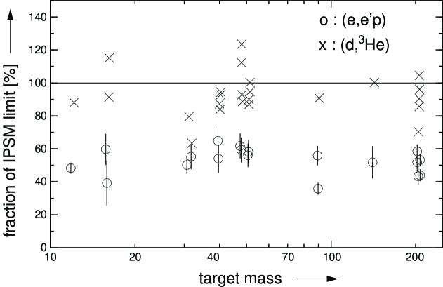
Figure 1: Spectroscopic strength relative to the Independent-Particle Shell Model limit for valence orbitals as a function of the mass number according to literature values for (d,³He) and (e,e^′p) experiments. For references see Table 3.

Modern nuclear-structure calculations [5, 6, 7, 8, 9, 10, 12, 11] predict occupations for valence orbitals in the range of 60 to 90 % of the IPSM limit. The precise value and the spreading of the strength depend sensitively on the amount of short- and long-range correlations included in the calculation. Recently, it was demonstrated [14] for the nucleus ⁷Li that structure calculations based on a realistic nucleon-nucleon potential are indeed able to describe accurately the momentum distributions and spectroscopic factors measured with the reaction (e,e^′p). To put such calculations to a further test for other nuclei it is necessary to avail of accurate absolute spectroscopic factors. In this respect the existing discrepancy between spectroscopic factors deduced from the (e,e^′p) and (d,³He) reactions needs a detailed investigation. It is the aim of the present paper to carry out such a study and to provide a consistent set of spectroscopic factors extracted from both the (e,e^′p) and the (d,³He) reaction.

In Section 2 the Coulomb Distorted Wave Impulse Approximation (CDWIA), which is used in the analysis of the (e,e^′p) experiments, and the Distorted Wave Born Approximation (DWBA) method, used for the (d,³He) reaction, are reviewed with special emphasis on the sensitivities of the spectroscopic factors to the various approximations made. In Section 3 it is investigated, which part of the bound-state wave function (BSWF) is probed by the (e,e^′p) and (d,³He) reactions, in order to understand the model sensitivity arising from the shape of the BSWF. In Section  4 one ⁴⁸Ca(e,e^′p) [13] and two ⁴⁸Ca(d,³He) [15, 16] data sets are used for a detailed comparison between the (e,e^′p) and (d,³He) spectroscopic factors. In Section  5 a re-analysis of (d,³He) data sets for other nuclei is made, in which non-locality and finite range corrections are included and BSWF’s deduced from (e,e^′p) experiments are used. Conclusions are drawn in Section 6.

2 Description of the reactions (e,e^′p) and (d,³He)

2.1 The (e,e^′p) reaction

In (e,e^′p) experiments the energy ${e_{i}}$ and momentum $\vec{k}_{i}$ of the initial electron, and the energies and momenta of the final electron and knocked-out proton, denoted by ${e}_{f}$, $\vec{k}_{f}$ and ${E}_{p}$, $\vec{k}_{p}$, respectively, are measured. The energy and momentum transferred by the scattered electron are denoted by : $\omega={e}_{i}-{e}_{f}$ and $\vec{q}=\vec{k}_{i}-\vec{k}_{f}$. From energy and momentum conservation the missing energy $E_{m}$ and missing momentum $\vec{p}_{m}$ are determined :

$${E}_{m}={e}_{i}-{e}_{f}-{E}_{p}-{T}_{A-1}=\omega-{E}_{p}-{T}_{A-1}$$

$$\vec{p}_{m}=\vec{k}_{p}^{lab}-(\vec{k}_{i}-\vec{k}_{f})=\vec{k}_{p}-\vec{q},$$ (1)

where $T_{A-1}$ is the kinetic energy of the residual nucleus.

The missing energy is the energy required to separate the struck proton from the target nucleus, where the final nucleus is left in the ground-state or in one of its excited states. The missing momentum is, according to the definition of Eq. (1), the proton momentum in the nucleus just before the reaction provided that there is no further interaction between the incoming electron and the initial nucleus and the outgoing electron and proton and the final nucleus.

In the plane-wave impulse approximation (PWIA, see below) the (e,e^′p) cross section can be written as :

$${{\rm d}^{6}\sigma\over{\rm d}E_{e\prime}{\rm d}\Omega_{e\prime}{\rm d}E_{p}{\rm d}\Omega_{p}}={k}\sigma_{ep}S(E_{m},\vec{p}_{m}),$$ (2)

where the left-hand side represents the measured (e,e^′p) cross section, $k\sigma_{ep}$ a kinematic factor times the elementary electron-proton cross section and $S$($E_{m}$,$\vec{p}_{m}$) the spectral function [17, 18, 19, 20]. The spectral function is the joint probability of finding a proton with momentum $\vec{p}_{m}$ and binding energy $E_{m}$ inside the nucleus. For a transition leading to a discrete state at $E_{m}$=$E_{tr}$, the spectral function is written as the momentum distribution $\rho$($\vec{p}_{m}$) times a delta function for the energy :

$$S(E_{m},\vec{p}_{m})=\rho(\vec{p}_{m})\delta(E_{m}-{E}_{tr}).$$ (3)

The spectral function as given in Eq. (2) cannot be determined experimentally because the outgoing proton interacts strongly with the final nucleus (this is often called the Final State Interaction, FSI). Moreover the factorization of the six-fold differential cross section into an elementary electron-proton cross section times the spectral function does not hold any more due to the FSI and Coulomb distortions of the electron waves.

In the following a theoretical basis similar to the one used in the description of the (d,³He) reaction is given to compute the (e,e^′p) cross section, in which the interaction between the participating particles is taken into account. The influence of various approximations made in this analysis is also investigated in order to reveal the origin of the model uncertainties on the extracted observables. Since we want to keep the formulae transparent the angular momentum and spin parts are not given in this article.

The basis of the theoretical description of the reaction : $A+e_{i}\rightarrow B+p+e_{f}$ is the T-matrix formalism [21, 22, 23]. This T-matrix in the prior form is defined in the following way :

$$T_{if}~{}=~{}<\Psi^{(-)}_{f}~{}|V_{i}-U_{i}|~{}\psi_{A}~{}\varphi^{(+)}_{i}>,$$ (4)

where $\varphi^{(+)}_{i}(\vec{k}_{i},\vec{r}\,)$ is the incoming distorted electron wave with outgoing-wave boundary conditions, $\psi_{A}$ the wave function of the target nucleus, $V_{i}$ the total interaction between the incoming electron and the nucleus, from which $U_{i}$, the potential used to generate the distorted wave $\varphi_{i}$, is excluded, and $\Psi^{(-)}_{f}$ is the exact final-state wave function of the electron-proton-residual-nucleus system obeying incoming-wave boundary conditions. The distorting potential $U_{i}$ is usually taken to be the Coulomb potential arising from a uniformly charged sphere.

In the distorted-wave approximation the exact final-state wave function is approximated by the product of an internal wave function for the residual nucleus $\psi_{B}$, a distorted outgoing electron-wave $\varphi^{(-)}_{f}(\vec{k}_{f},\vec{r}\,)$, and the distorted outgoing proton-wave $\chi^{(-)}_{p}(\vec{k}_{p},\mu\vec{R}\,)$ (with $\mu=(A-1)/A$). Here the displacement of the knocked-out proton from the residual nucleus $B$ is denoted by $\vec{R}$, while $\vec{r}\,$ is the displacement of the electron from the center of mass of the residual-nucleus plus proton final system (see Fig. 2a). Under these assumptions the distorted wave transition amplitude becomes :

$$T^{DW}_{if}=~{}<\varphi^{(-)}_{f}(\vec{k}_{f},\vec{r}\,)~{}\chi^{(-)}_{p}(\vec{k}_{p},\mu\vec{R}\,)~{}\psi_{B}~{}|V_{i}-U_{i}|~{}\psi_{A}~{}\varphi^{(+)}_{i}(\vec{k}_{i},\vec{r}\,)>.$$ (5)

For light and medium-heavy nuclei the effects of the electron distortions are small [24]; for heavy nuclei, however, these effects become sizable. Because of the long range of the Coulomb potential it is difficult to include electron distortions in theoretical codes that compute (e,e^′p) momentum distributions. Up to now two approaches have been followed to deal with these distortions. In the simplest one, the Effective Momentum Approximation (EMA) [25], the electron momenta are replaced by effective ones. A more precise treatment of the electron distortions is employed in the work of Giusti and Pacati [26, 27], in which the eikonal approach is used to expand the electron waves in powers of $Z\alpha$ ($Z$ the nuclear charge and $\alpha$ the fine-structure constant). For medium heavy nuclei such as the calcium isotopes this approximation is accurate enough as all higher order terms have negligible influence on the calculated cross sections [27]. Recently, full relativistic calculations [28, 29, 30] have been used to analyze momentum distributions measured with the reaction (e,e^′p). The deduced spectroscopic factors are different by up to 10% from those resulting from a non-relativistic analysis. However, in these analyses relativistic Hartree-Fock wave functions are used for the BSWF, which not always provide a satisfactory description of the experimental momentum distributions. Moreover, the use of relativistic optical potentials at the low proton energies ($T_{p}\leq$ 100 MeV) employed in the presently discussed experiments may be questionable. We therefore limit the present analysis to the non-relativistic approach.

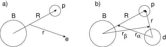
Figure 2: The geometry used in the description of the (e,e^′p) reaction (a) and the (d,³He) reaction (b).

The distorted proton wave, $\chi^{(-)}_{p}(\vec{k}_{p},\mu\vec{R}\,)$, is usually chosen to be the solution of the Schrödinger equation with the optical potential that describes elastic proton scattering off the final nucleus, $B$. The parameterization of the optical potential is not unique; using a different parameterization to generate the distorted proton waves results in waves identical at large distances but different in the nuclear region where the (e,e^′p) reaction takes place. The effect of different parameterizations on the value of the extracted spectroscopic factors has been investigated for the reaction ⁵¹V(e,e^′p) [2]. A model uncertainty of about 6 % was found there due to the treatment of the final-state interaction.

The optical potential used for the generation of the distorted waves as well as the binding potential for the proton are local potentials. However, for fundamental reasons this potential is expected to be non-local. Perey [31] has pointed out that the wave function of a non-local potential is systematically smaller in the nuclear interior than the wave function of the local potential that gives an equivalent description of the elastic scattering process. This non-locality correction can be taken into account effectively by multiplying the local wave function with the factor :

$$F(r)=\bigl{(}1-{{\mu_{p}\beta^{2}}\over{2\hbar^{2}}}U_{L}(r)\bigr{)}^{-1/2},$$ (6)

where $\mu_{p}={{A-1}\over A}m_{p}$ is the reduced proton mass, $U_{L}(r)$ the local optical potential and $\beta$ the range of the non-locality. The non-locality correction affects the distorted waves in the region where the potential is significantly different from zero. This is also the region where the reaction takes place so that the non-locality correction also affects the spectroscopic factors determined from knock-out reactions.

The T-matrix element $T^{DW}_{if}$ can be written in a way that explicitly shows the nuclear-structure part :

$$T^{DW}_{if}=~{}\int d\vec{r}\int d\vec{R} \varphi^{(-)*}_{f}(\vec{k}_{f},\vec{r}\,)~{}\chi^{(-)*}_{p}(\vec{k}_{p},\mu\vec{R}\,)\times$$ (7)

$$<\psi_{B}|V_{i}-U_{i}|\psi_{A}>\varphi^{(+)}_{i}(\vec{k}_{i},\vec{r}\,).$$

The matrix element $<\psi_{B}|V_{i}-U_{i}|\psi_{A}>$ contains the nuclear-structure information. It involves integration over all internal coordinates $\xi_{B}$, independent of $\vec{r}$ and $\vec{R}$. The potential $V_{i}$ describes the total interaction between the electron and the nucleus, whereas in the distorting potential $U_{i}$ the part of the interaction leading to the (e,e^′p) channel is excluded. In this way the difference $V_{i}-U_{i}$ is the interaction between the electron and the struck proton :

$$V_{i}-U_{i}=V_{ep}(\vec{r},\mu\vec{R}\,).$$ (8)

Since $V_{ep}$ is independent of the internal coordinates of $\psi_{B}$, the nuclear matrix element can be factorized into $V_{ep}$ and the nuclear overlap integral :

$$<\psi_{B}|V_{i}-U_{i}|\psi_{A}>~{}=~{}V_{ep}(\vec{r},\mu\vec{R}\,)\int d\xi_{B}~{}\psi^{*}_{B}(\xi_{B})\psi_{A}(\xi_{B},\vec{R}\,).$$ (9)

The integral is usually expanded into single-particle states [21] :

$$\int d\xi_{B}\psi^{*}_{B}(\xi_{B})\psi_{A}(\xi_{B},\vec{R}\,)=\sum_{n\ell jm}\!<J_{B}jM_{B}m|J_{A}M_{A}>\!\sqrt{S_{n\ell j}}~{}\phi_{n\ell jm}(\vec{R}\,),$$ (10)

where $<\!J_{B}jM_{B}m|J_{A}M_{A}\!>$ is a Clebsch-Gordan coefficient, $\sqrt{S_{n\ell j}}$ the spectroscopic amplitude and $\phi_{n\ell jm}(\vec{R}\,)$ a normalized single particle wave function, usually referred to as the bound state wave function (BSWF). Substituting the foregoing two expressions into the transition amplitude yields :

$$T^{CDWIA}_{if}= \sum_{n\ell jm}\!<J_{B}jM_{B}m|J_{A}M_{A}>\!\sqrt{S_{n\ell j}}\int d\vec{r}\int d\vec{R}\varphi^{(-)*}_{f}(\vec{k}_{f},\vec{r}\,)\times$$ (11)

$$\chi^{(-)*}_{p}(\vec{k}_{p},\mu\vec{R}\,)V_{ep}(\vec{r},\mu\vec{R}\,)~{}\phi_{n\ell jm}(\vec{R}\,)~{}\varphi^{(+)}_{i}(\vec{k}_{i},\vec{r}\,),$$

which is the Coulomb Distorted Wave Impulse Approximation (CDWIA) amplitude. In the code DWEEPY [27] that was used to calculate the momentum distributions presented in Section 4, this expression is evaluated together with the angular momentum and spin parts, which are not shown in Eq. (11). From Eq. (11) the Distorted-Wave Impulse Approximation (DWIA) amplitude is obtained by replacing the electron waves by plane waves :

$$T^{DWIA}_{if}= \sum_{n\ell jm}\!<J_{B}jM_{B}m|J_{A}M_{A}>\!\sqrt{S_{n\ell j}}\int d\vec{r}\int d\vec{R}\exp(-i\vec{k}_{f}\!\cdot\!\vec{r}\,)\times$$ (12)

$$\chi^{(-)*}_{p}(\vec{k}_{p},\mu\vec{R}\,)V_{ep}(\vec{r},\mu\vec{R}\,)~{}\phi_{n\ell jm}(\vec{R}\,)~{}\exp(i\vec{k}_{i}\!\cdot\!\vec{r}\,).$$

In order to gain some further insight into Eq. (12) and to make the connection with the PWIA expression the Coulomb potential is now used for the interaction : $V_{ep}=\alpha/|\mu\vec{R}-\vec{r}\,|$. With this potential the integration over $\vec{r}\,$ can be performed :

$$T^{DWIA}_{if}= \sum_{n\ell jm}\!<J_{B}jM_{B}m|J_{A}M_{A}>\!{{4\pi\alpha}\over{\vec{q}\,^{2}}}\sqrt{S_{n\ell j}}\times$$ (13)

$$\int d\vec{R}~{}\exp(-i\vec{q}\!\cdot\!\mu\vec{R}\,)~{}\chi^{(-)*}_{p}(\vec{k}_{p},\mu\vec{R}\,)~{}\phi_{n\ell jm}(\vec{R}\,),$$

where $\vec{q}=\vec{k}_{i}-\vec{k}_{f}$. The Plane-Wave Impulse Approximation (PWIA) amplitude is obtained from the expression (13) by replacing the distorted proton waves by plane waves :

$$T^{DWIA}_{if}=\sum_{n\ell jm}\!<J_{B}jM_{B}m|J_{A}M_{A}>\!\sqrt{S_{n\ell j}}\times~{}~{}~{}~{}~{}~{}~{}~{}~{}~{}~{}~{}~{}~{}~{}~{}~{}~{}~{}~{}~{}~{}~{}~{}~{}~{}$$

$$\int d\vec{R}~{}\exp(i\vec{q}\!\cdot\!\mu\vec{R}\,)\exp(-i\vec{k}_{p}\!\cdot\!\mu\vec{R}\,)~{}\phi_{n\ell jm}(\vec{R}\,)~{}~{}~{}~{}~{}~{}~{}~{}~{}~{}~{}~{}~{}$$

$$=\sum_{n\ell jm}\!<J_{B}jM_{B}m|J_{A}M_{A}>\!\sqrt{S_{n\ell j}}\int d\vec{R}~{}\exp(-i\vec{p}_{m}\!\cdot\!\vec{R}\,)~{}\phi_{n\ell jm}(\vec{R}\,),$$ (14)

where in the last expression the proton momentum $\vec{k}_{p}$, which is the center-of-mass momentum, has been written in terms of laboratory momenta : $\vec{k}_{p}=\vec{k}_{p}^{lab}+\vec{p}_{m}/(A-1)$. Expression (14) is just the Fourier transform of the BSWF. After including the angular momentum and spin parts and squaring the $T_{if}$-matrix element the well known expression [17] for the (e,e^′p) cross section is obtained.

When distortions (of the proton or electron waves) are included, the cross section cannot be factorized any more into $\sigma_{ep}$ and S($E_{m}$,$\vec{p}_{m}$) (see Eq. (2)). For convenience one defines the reduced cross section or distorted momentum distribution (both the experimental and the calculated one) by

$$\rho^{D}(\vec{p}_{m})\delta(E_{m}-{E}_{tr})=S^{D}(E_{m},\vec{p}_{m})=\frac{1}{{k}\sigma_{ep}}\frac{{\rm d}^{6}\sigma^{CDWIA}}{{\rm d}E_{e\prime}{\rm d}\Omega_{e\prime}{\rm d}E_{p}{\rm d}\Omega_{p}}$$ (15)

(compare eqs. 2 and 3). In calculating the sixfold differential cross section there is some ambiguity in the current operator to be used as the proton is off-shell [32, 33, 34]. However, in the used kinematics the influence on the spectroscopic factors of the different prescriptions as given by de Forest [32] is smaller than a few percent.

2.2 The (d,³He) reaction

The basis of the DWBA description [21, 22, 23] of transfer reactions $A+a\rightarrow B+b$, such as the (d,³He) reaction presently under study, is the transition amplitude :

$$T_{\alpha\beta}\,=\,<\!\Psi^{(-)}|V_{\alpha}-U_{\alpha}|\psi_{A}\psi_{a}\chi^{(+)}_{\alpha}(\vec{k}_{\alpha},\vec{r}_{\alpha})\!>,$$ (16)

where $\alpha~{}(\beta)$ is the entrance (exit) channel with projectile (ejectile) $a~{}(b)$ and target (final) nucleus $A~{}(B\,)$ and $\vec{r}_{\alpha}$ the displacement of $a$ from $A$ (see Fig. 2b). The interaction $V_{\alpha}$ is the sum of two-body interactions between the nucleons of the projectile and those of the target nucleus. The wave function $\psi_{a}~{}(\psi_{A})$ is the internal wave function of the projectile (target nucleus), while $\chi^{(+)}_{\alpha}(\vec{k}_{\alpha},\vec{r}_{\alpha})$ is the solution of the Schrödinger equation for the incoming particle with the distorting potential $U_{\alpha}$, usually chosen to be an optical potential that fits the elastic scattering in channel $\alpha$, and $\Psi^{(-)}$ is the exact wave function of the system with incoming-wave boundary conditions.

In the DWBA method the following approximations are made : First the exact wave function $\Psi^{(-)}$ is replaced by a product of internal wave functions of the outgoing particle $\psi_{b}$, the residual nucleus $\psi_{B}$ and a function $\chi^{(-)}_{\beta}(\vec{k}_{\beta},\vec{r}_{\beta})$ describing the elastic scattering of the outgoing particle off the final nucleus B. This leads to the distorted-wave transition amplitude :

$$T^{DW}_{\alpha\beta} = <\!\chi^{(-)}_{\beta}(\vec{k}_{\beta},\vec{r}_{\beta})~{}\psi_{b}\psi_{B}|V_{\alpha}-U_{\alpha}|\psi_{A}\psi_{a}~{}\chi^{(+)}_{\alpha}(\vec{k}_{\alpha},\vec{r}_{\alpha})\!>$$

$$= \!\int\!d\vec{r}_{\beta}\int\!d\vec{r}_{\alpha}~{}\chi^{(-)*}_{\beta}(\vec{k}_{\beta},\vec{r}_{\beta})<\!Bb|V_{\alpha}-U_{\alpha}|Aa\!>\chi^{(+)}_{\alpha}(\vec{k}_{\alpha},\vec{r}_{\alpha}),$$ (17)

where $\vec{r}_{\beta}$ is the displacement of $b$ from $B$ (see Fig. 2a). In the nuclear matrix element $<\!\psi_{b}\psi_{B}|V_{\alpha}-U_{\alpha}|\psi_{A}\psi_{a}\!>$ the integration is performed over all coordinates independent of $\vec{r}_{\alpha}$ and $\vec{r}_{\beta}$.

The second approximation deals with the interaction $V_{\alpha}-U_{\alpha}$, which is replaced in the prior formalism by the interaction between the transferred nucleon and the projectile nucleons :

$$V_{\alpha}-U_{\alpha}\approx\sum_{i}^{a}V_{in}\,=\,V_{an}(\vec{r}\,),$$ (18)

where the sum runs over all the constituents of the projectile $a$, $n$ is the nucleon to be transferred and $\vec{r}\,$ is the displacement of the pickup nucleon from the center of mass of the projectile. (In principle this interaction should be taken off-shell. In view of the many other approximations made, this point is probably not relevant and is always neglected in analyses.)

The above approximations are based on the following assumptions made for the transfer reaction mechanism itself. Firstly it is assumed that the interaction that drives the reaction is weak enough so that the reaction process may be treated in first order perturbation theory. Secondly the reaction is assumed to be a one-step process; the transferred nucleon is picked up by the incoming projectile, whereas all other target nucleons do not change their state of motion.

The distorted waves, $\chi^{(+)}_{\alpha}(\vec{k}_{\alpha},\vec{r}_{\alpha})$ and $\chi^{(-)}_{\beta}(\vec{k}_{\beta},\vec{r}_{\beta})$, are usually chosen to be the wave functions of optical potentials describing elastic scattering in the entrance and exit channels. However, as already mentioned, the same elastic scattering data can be described with different parameterizations of the optical potential, resulting in waves identical at large distances but differing in the nuclear region. Their contribution to the transition amplitude will differ accordingly and gives rise to an extra uncertainty in the spectroscopic factors deduced from transfer reactions. In contrast to the (e,e^′p) reaction where only one wave function enters that is generated in an optical model potential, in the (d,³He) reaction two such wave functions are entering. Moreover, the uncertainty in the optical-model wave functions of composite particles in the interior of the nucleus is appreciably larger than that for nucleons. Consequently, the uncertainties due to different possible parameterizations of the optical-model potential are larger for spectroscopic factors deduced from the (d,³He) reaction.

As pointed out earlier, non-locality corrections must be applied to the wave functions obtained from the (local) optical potential. This correction affects the wave functions of the projectile and ejectile in the region where the transfer takes place.

The nuclear matrix element in Eq. (17) can be expanded, along the lines given in [23], into the nuclear overlap integral as given in Eq. (10) and into the overlap between the projectile and ejectile : $f(\vec{r}\,)~{}=~{}<\psi^{*}_{b}(\xi_{a},\vec{r}\,)|V_{an}(\vec{r}\,)|\psi_{a}(\xi_{a})>$. This gives for the DWBA transition amplitude :

$$T^{DW}_{\alpha\beta}\propto\sum_{n\ell jm}\!\sqrt{S_{n\ell j}}\!\int d\vec{r}_{\beta}\!\int d\vec{r}_{\alpha}~{}\chi^{(-)*}_{\beta}(\vec{k}_{\beta},\vec{r}_{\beta})\phi_{n\ell jm}(\vec{R}\,)f(\vec{r}\,)\chi^{(+)}_{\alpha}(\vec{k}_{\alpha},\vec{r}_{\alpha}).$$ (19)

The evaluation of this amplitude involves a six-dimensional integral over $\vec{r}_{\alpha}$ and $\vec{r}_{\beta}$. A reduction to a more convenient three-dimensional integral is achieved in the zero-range approximation, where the effective interaction $V_{an}(\vec{r}\,)$ is assumed to have a range equal to zero, so that

$$f(\vec{r}\,)\, = D_{0}\delta(\vec{r}\,),$$

$$D_{0} = \int{\rm d}\vec{r}\ <\psi^{*}_{b}(\xi_{a},\vec{r}\,)|V_{an}(\vec{r}\,)|\psi_{a}(\xi_{a})>.$$ (20)

The physical meaning of this approximation is that the ejectile $b$ is assumed to be emitted at the same position where the absorption of the projectile $a$ has taken place. The effect of neglecting the finite range of the interaction is that the spectroscopic factors deduced from transfer reactions in a zero-range analysis are larger than the ones obtained from a full finite-range analysis [4].

Full finite-range calculations are hard to perform because of the six dimensional integral in Eq. (19). However it has been shown by Buttle and Goldfarb [35] that the effects of the finite range of the interaction can be taken into account approximately (local energy approximation, LEA) by replacing the delta function in Eq. 20 by the following radial factor :

$$\Lambda(r)=[1\!+\!{{2m_{a}m_{p}}\over{\hbar^{2}m_{b}}}R_{fr}^{2}({E}_{\alpha}-U_{\alpha}(\mu r)+{E}_{p}-U_{p}(r)-{E}_{\beta}+U_{\beta}(r))]^{-1},$$ (21)

in which $R_{fr}$ is the finite range distance.

3 BSWF probing functions

As shown in Section 2, the transition amplitudes of both the (e,e^′p) and (d,³He) reaction consist of the nuclear matrix element sandwiched between the incoming and outgoing distorted ”probing” waves (see eqs. (7) and (17)). In this section it is investigated to which part of the BSWF the (e,e^′p) reduced cross section and the (d,³He) cross section are sensitive.

Cross sections are obtained from the T-matrix elements by integrating the radial coordinate from zero to infinity. The radial sensitivity of the cross section was investigated by varying the lower radial integration bound between 0 and 10 fm and plotting these results as :

$$P(r)={1\over{\Delta r}}(\sigma_{r-\Delta r/2}-\sigma_{r+\Delta r/2}),$$ (22)

where $\sigma_{x}$ reperesents the cross section calculated with a lower limit $x$ on the integral over the T-matrix element :

$$\sigma_{x}\propto|\int_{x}^{\infty}T(r)~{}{\rm d}r|^{2}.$$ (23)

In this way the separate contribution of the interval $\Delta r$ around $r$ to the cross section was obtained and hence the part of the BSWF to which the reaction is sensitive can be determined.

For the reaction ⁴⁸Ca(e,e^′p) these calculations were performed for the transitions leading to the 1/2⁺ ground-state and the first 3/2⁺ excited state in ⁴⁷K. The BSWF shown in the upper part of Fig. 3 that was used in these calculations was generated in a Woods-Saxon well with the parameters as given in Section 4. In that section the other parameters that entered these CDWIA calculations are also given. The results of the calculation of $P(r)$ for the (e,e^′p) reaction are shown in the middle part of Fig. 3 for different values of the missing momentum. From this figure it can be seen that the (e,e^′p) reaction is sensitive to the whole BSWF and the largest contribution to the momentum distribution comes from those regions in $r$, where also $r^{2}\Phi_{nlj}(r)$ is large. For the 1d_3/2 orbital this is the region between r=2.5 and 4.5 fm and for the 2s_1/2 orbital between r=0.7 and 6.7 fm. Because of the node in the 2s_1/2 orbital, for low missing momenta, there is a destructive contribution to the momentum distribution from the inner lobe, whereas this contribution becomes constructive for high missing momenta.

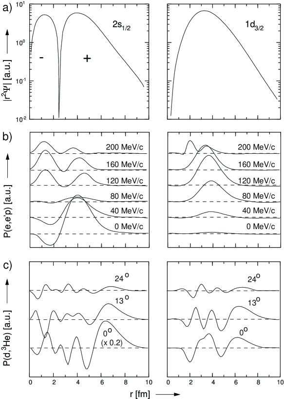
Figure 3: a) The BSWF as obtained from the present (e,e^′p) experiment for the 1d_3/2 and 2s_1/2 orbitals. b) The sensitivity P (see text) of the (e,e^′p) momentum distributions to these BSWF. c) The sensitivity P (see text) of the (d,³He) differential cross sections to these BSWF.

For the above mentioned transitions the sensitivity to the BSWF was also determined for the (d,³He) reaction. The DWBA calculations were performed with the parameters as given in Section 4 and the same BSWF as for the (e,e^′p) experiment was used. The results of these calculations are presented in the lower part of Fig. 3. Here it can be seen that apart from strong interferences between the incoming and outgoing distorted waves in the interior of the nucleus, the (d,³He) reaction is most sensitive to the region between $r$=5 and 10 fm. Therefore, the (d,³He) reaction is not sensitive to the details of the BSWF inside the nucleus. In the region where the (d,³He) reaction is sensitive the BSWF has the global form : $\nu\exp(-\kappa r)$, where $\kappa$ depends on the (measured) binding energy of the proton, and the normalization $\nu$ depends on the depth and shape of the potential that generates the BSWF. As the spectroscopic factor is the integral of the BSWF over the total radial region, one can only determine spectroscopic factors from the (d,³He) reaction by assuming some shape for the BSWF.

The conclusion is that with the (e,e^′p) reaction the BSWF is probed in the whole radial region whereas, with the (d,³He) reaction only the exponential tail of the BSWF is probed. This tail is very sensitive to the exact shape of the used proton-binding potential. The shape of the BSWF introduces thus a large model dependence, sometimes up to 50% [4], in spectroscopic factors deduced from (d,³He) experiments.

Given this sensitivity, it is even questionable whether ratios of spectroscopic factors for different isotopes can be determined accurately in the (d,³He) reaction [36], as it is not certain that the radius of the BSWF well scales with A^1/3.

4 Analysis of the ⁴⁸Ca data

4.1 Analysis of the ⁴⁸Ca(e,e^′p) experiment

The experimental (e,e^′p) momentum distributions were obtained with the coincidence set-up at NIKHEF [37]. Two metal foils with a thicknesses of 7.3 and 15.0 mg/cm², enriched to 95.2 % in ⁴⁸Ca were used. Reduced cross sections were obtained under parallel kinematic conditions in the range between -60 and 260 MeV/c. The electron beam energy was 440 MeV and the outgoing proton kinetic energy was 100 MeV. The experimental systematic error on the extracted distributions is 4 %. Further details can be found in Ref. [13]. The CDWIA calculations were performed with the code DWEEPY [27]. The proton optical-potential parameters were obtained from the work of Schwandt et al. [38]. A non-locality correction according to the prescription of Perey [31] (see also Eq. (6)) was applied with a range parameter $\beta$ of 0.85 fm. The bound state wave function was calculated in a Woods-Saxon well with a diffuseness $a_{0}$ of 0.65 fm and a Thomas spin-orbit parameter $\lambda$ of 25. A non-locality correction was also applied to the BSWF with a $\beta_{nloc}$ of 0.85 fm. The well depth $V_{0}$ and the radius parameter r₀ were adjusted with the separation energy as a constraint to get the best description of the measured momentum distributions. In Fig. 4 these reduced cross sections are shown for the transitions to the first three positive parity states together with the results of the CDWIA calculations, while in Table 1 the deduced spectroscopic factors and radii of the BSWF are given.

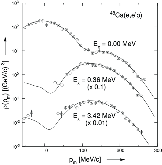
Figure 4: Momentum distributions for the first three positive-parity transitions in the reaction ⁴⁸Ca(e,e^′p) together with curves obtained from the CDWIA calculations as mentioned in the text.

Table 1: Spectroscopic factors for proton pick up from ⁴⁸Ca deduced from (e,e^′p) and from (d,³He) experiments.

$E_{x}$	$J^{\pi}$	$r_{0}$	$r_{\rm rms}$ +)	$S$ (e,e′p)	S(d,3He)[15]		$S$(d,3He)[16]
[MeV]		[fm]	[fm]		LZR	NLFR	NLFR
0.00	$1/2^{+}$	1.228(47)	3.58(10)	1.07 ( 7)	1.55	0.96	0.94(25)
0.36	$3/2^{+}$	1.254(48)	3.54(10)	2.26 (16)	4.16	2.39	2.31(65)
3.42	$5/2^{+}$	1.128(44)	3.39( 9)	0.683(49)	1.02	1.28	1.07(31)
3.85	$1/2^{+}$	1.294(51)	3.59(10)	0.167(14)	0.28	0.12
3.95	$3/2^{+}$	1.288	3.54	0.323(27)	0.70	0.32
5.24	$5/2^{+}$	1.192(48)	3.49( 8)	0.288(21)	0.32	0.27
5.49	$5/2^{+}$	1.182(46)	3.47( 9)	0.746(52)	0.94	0.84
6.51	$5/2^{+}$	1.265(56)	3.62(12)	0.160(14)	0.22	0.11
6.87	$5/2^{+}$	1.162(65)	3.41(14)	0.070( 7)	0.14	0.14
7.81	$5/2^{+}$	1.243(49)	3.56( 9)	0.434(32)	0.71	0.42
8.13	$5/2^{+}$	1.299(54)	3.46(12)	0.228(19)	0.33	0.26
+) rms radius in the proton A-1 system.

4.2 Re-analysis of the ⁴⁸Ca(d,³He) experiments

For the comparison with the data from the (e,e^′p) experiment a re-analysis of two ($\vec{\rm d},^{3}$He) experiments was performed. The first (d,³He) experiment [15] was performed with an incoming deuteron energy of 79.2 MeV. Further details of this experiment can be found in the original paper [15]. In the analysis in that paper a local zero-range DWBA calculation was used for the extraction of the spectroscopic factors together with a BSWF potential well with $r_{0}$=1.25 fm, $a_{0}$=0.60 fm and $V_{0}$ adjusted to get the correct binding energy. Non-locality corrections were not applied to the BSWF. The ratio of the spectroscopic factors given in [15] to those deduced from the present (e,e^′p) experiment for several discrete states is shown in Fig. 5a as a function of the excitation energy. The (d,³He) spectroscopic factors calculated this way are on the average 50% higher than those obtained from the (e,e^′p) experiment.

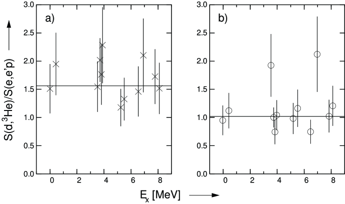
Figure 5: a) The ratio of the spectroscopic factors given in Ref. [15] derived from a local zero-range analysis of the ⁴⁸Ca(d,³He) experiment and those obtained from the present ⁴⁸Ca(e,e^′p) experiment for various transitions observed in both reactions as a function of excitation energy. The solid line represents the average. b) The same ratio after including non-locality and finite-range corrections in the (d,³He) analysis and using the BSWF’s obtained from the (e,e^′p) experiment. A 30% error was assigned to the (d,³He) spectroscopic factors in both cases.

In the present re-analysis, performed with the code DWUCK4 [41], non-locality corrections and finite range corrections via the LEA approach were included together with the BSWF obtained from the present (e,e^′p) experiment. The same optical model parameter sets for the deuteron and ³He waves were used as in Ref. [15]. Spectroscopic factors deduced with this re-analysis are given in Table 1. In order to estimate realistic errors on the spectroscopic factors deduced from the (d,³He) experiment the following sources of uncertainties were taken into account : i) a total experimental systematic error of 5% which includes the error on the target thickness; ii) the effect of the uncertainty (about 3%) in the rms radii obtained from the (e,e^′p) experiment, which yields 25% for the transition to the 1/2⁺, 28% for the transition to the 3/2⁺ and 29% for the transition to the 5/2⁺state; iii) a 10% uncertainty due to the $<{\rm d}|^{3}$He$>$ overlap function (the value of $D_{0}$); and iv) at least a 10% uncertainty due to different possible parameterizations of the deuteron and ³He optical potentials. The latter number is taken from [4], where the sensitivity of the spectroscopic factors to different optical potential parameterizations was investigated for the reaction ⁵¹V(d,³He)⁵⁰Ti at 53 MeV.

The ratio of the spectroscopic factors obtained from the present analysis of the (d,³He) data to those obtained from the (e,e^′p) experiment is plotted in Fig. 5b. The average ratio is one, so it is concluded that, except for two points, there is a very good agreement between the spectroscopic factors obtained from both reactions. This agreement is obtained by including non-locality and finite-range corrections in the analysis together with experimental BSWF’s obtained from the (e,e^′p) experiment. Finite-range corrections reduce the spectroscopic factors by about 15 % and the use of the BSWF determined from the (e,e^′p) analysis gives a a further reduction of 30 to 40 %.

The deviation of the spectroscopic factors and the relatively small rms radius for the transition leading to the 3.42 MeV excited state in ⁴⁷K might be ascribed to some unresolved 1f_7/2 strength at 3.4 MeV [13] but in the scarce literature on the level scheme of ⁴⁷K no 7/2^- states have been reported so far. The reduced cross section for this transition can also be described well with a BSWF with an rms radius of 3.47 fm, which is the average value for the 1d_5/2 orbital obtained from all the 5/2⁺ transitions observed in the (e,e^′p) experiment. This gives a 3 % lower spectroscopic factor in the (e,e^′p) experiment, but in the (d,³He) analysis the spectroscopic factor drops by 14 %. The deviation for the spectroscopic factor for the very weak transition at 6.87 MeV may be due to the uncertainty in the rms radius that is not well determined from the (e,e^′p) experiment. It is also possible that two-step processes have a different effect on the (e,e^′p) and (d,³He) cross sections for this weak transition.

The second experiment was performed with an incoming deuteron energy of 56 MeV [16]. Angular distributions and asymmetries were measured for the first three positive parity transitions, leading to 1/2⁺, 3/2⁺and 5/2⁺ states in ⁴⁷K, see Fig. 6. The used optical-model potential parameterizations for the deuteron and ³He waves were obtained from elastic deuteron and ³He scattering off ⁴⁸Ca [39] and are listed in Table 2. The non-locality corrections were taken into account according to the prescription of Perey [31] (see also Eq. (6)). For the deuteron and ³He wave-functions the parameters are given in the last column of Table 2. The same BSWF as obtained in the analysis of the (e,e^′p) experiment was employed in the calculation of the (d,³He) cross sections.

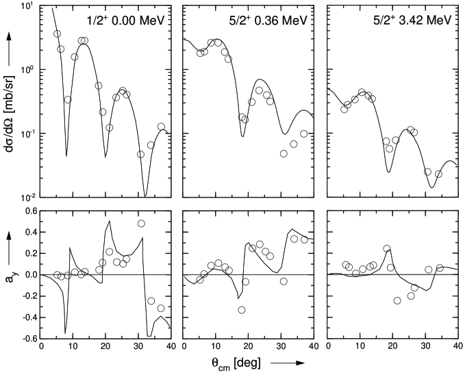
Figure 6: Angular distributions and asymmetries for the transitions leading to the first three positive-parity states in ⁴⁷K in the reaction ⁴⁸Ca(d,³He) at $E_{d}$ = 56 MeV.

Table 2: Optical potential parameters [39] for deuteron and ³He scattering off ${}^{48}\rm Ca$.

particle	$E_{\rm lab}$	$V_{r}$	$r_{0}$	$a_{0}$	$W_{v}$	$W_{d}$	$r_{i}$	$a_{i}$
	[MeV]	[MeV]	[fm]	[fm]	[MeV]	[MeV]	[fm]	[fm]
d	56.0	79.0	1.154	0.755	6.431	4.992	1.490	0.694
3He	45.0	184.6	1.115	0.713	-	21.95	1.217	0.812

particle	$V_{ls}$	$r_{ls}$	$a_{ls}$	$r_{c}$	$\beta_{\rm nloc}$
	[MeV]	[fm]	[fm]	[fm]	[fm]
d	7.60	0.986	0.777	1.30	0.54
3He	-	-	-	1.40	0.2

Finite-range effects were included by applying the LEA correction (Eq. (21)). A finite range distance of 0.77 fm was used together with the Bassel normalization [40] $D_{0}$=2.95 for the overlap between the deuteron and the ³He ejectile. The LEA approach was compared to full finite-range calculations performed with the code DWUCK5 [41]. In the latter calculations the D-state of the deuteron was included and a (d,³He) overlap function was used that yields $D_{0}$=2.95. The cross sections in the full finite range calculations were globally 10 to 15 % larger (and hence the spectroscopic factors smaller) than in the LEA calculation. As the used value of $D_{0}$ has also an uncertainty for convenience all DWBA calculations to be presented were performed in LEA and the presented spectroscopic factors were obtained from those. In Fig. 6 the results of DWBA calculations are shown for the transitions mentioned. Both angular distributions and asymmetries are described well with the used optical potentials and the BSWF’s obtained from the (e,e^′p) experiment. The spectroscopic factors extracted for these three transitions are given in Table 1. An estimate of the errors on the spectroscopic factors from this (d,³He) experiment gives typically numbers between 25 and 35 %.

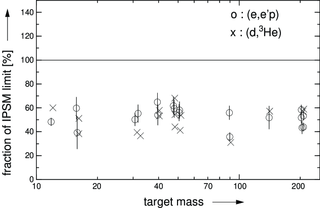
Figure 7: Summed spectroscopic strength of the valence orbit as function of the mass number normalized to the Independent-Particle Shell Model limit according to literature values from (e,e^′p) experiments and from a re-analysis, as discussed in the text, of the (d,³He) data presented in Fig. 1.

Table 3: Spectroscopic factors deduced from the re-analysis of existing (d,³He) data.

target	$E_{x}$	$J^{\pi}$	$S$ (e,e′p)	$r_{0}$	$S$ (d,3He)	$S$ (d,3He)
nucleus	[MeV]			[fm]	literature	re-analysis
12C	0.000	3/2-	1.72 (11) [42]	1.35 (2)	2.98 [43]	1.72
	2.125	1/2-	0.26 (  2)	1.65 (2)	0.69	0.27
	5.020	3/2-	0.20 (  2)	1.51 (2)	0.31	0.11
16O	0.000	1/2-	1.27 (13) [44]	1.37 (3)	2.30 [45]	1.02
	6.320	3/2-	2.25 (22)	1.28 (2)	3.64	1.94
31P	0.000	0+	0.40 (  3) [46]	1.27 (2)	0.62 [47]	0.36
	2.239	2+	0.60 (  5)	1.18 (3)	0.72	0.49
	3.498	2+	0.28 (  2)	1.12 (3)	0.30	0.19
40Ca	0.000	3/2+	2.58 (19) [48]	1.30 (5)	3.70 [49]	2.30
	2.522	1/2+	1.03 (  7)	1.28 (6)	1.65	1.03
51V	0.000	7/2-	0.37 (  3) [2]	1.30 (3)	0.73 [50]	0.30 [4]
	1.554	7/2-	0.16 (  2)	1.31 (4)	0.39	0.15
	2.675	7/2-	0.33 (  3)	1.32 (3)	0.64	0.26
	3.199	7/2-	0.49 (  4)	1.34 (3)	1.05	0.39
	4.410	1/2+	0.28 (  3)	1.22 (3)	0.63	0.22
	6.045	1/2+	0.35 (  3)	1.27 (4)	1.10	0.30
90Zr	0.000	1/2-	0.72 (  7) [2]	1.32 (3)	1.80 [51]	0.60 [52]
	0.909	9/2+	0.54 (  5)	1.31 (2)	1.25	0.30
	1.507	3/2-	1.86 (14)	1.27 (2)	3.90	1.20
	1.745	5/2-	2.77 (19)	1.30 (2)	8.90	2.40
142Nd	0.000	5/2+	1.39 (23) [53]	1.29 (9)	2.53 [54]	1.25
	0.145	7/2+	3.14 (43)	1.26 (8)	6.28	3.79
	1.118	11/2-	0.56 (  7)	1.28 (8)	0.74	0.36
	1.300	1/2+	0.05 (  1)	1.26 (9)	0.11	0.07

Table 4: Spectroscopic factors (continued from Table 3)

target	$E_{x}$	$J^{\pi}$	$S$ (e,e′p)	$r_{0}$	$S$ (d,3He)	$S$ (d,3He)
nucleus	[MeV]			[fm]	literature	re-analysis
206Pb	0.000	1/2+	0.68 (  6) [55]	1.23 (9)	1.15 [56]	1.03
	0.203	3/2+	1.10 (  9)	1.27 (9)	1.77	0.99
	0.616	5/2+	0.32 (  3)	1.23 (8)	0.52	0.44
	1.151	3/2+	0.52 (  5)	1.28 (9)	0.66	0.37
	1.479	11/2-	3.58 (32)	1.25 (9)	6.94	5.21
208Pb	0.000	1/2+	0.98 (  9) [55]	1.25 (8)	1.8   [57]	1.5
	0.350	3/2+	2.31 (22)	1.23 (8)	3.8	2.2
	1.350	11/2-	6.85 (68)	1.16 (9)	7.7	5.4
	1.670	5/2+	2.93 (28)	1.19 (8)	3.5	3.1
	3.470	7/2+	2.06 (20)	1.15 (9)	3.5	2.9

5 (d,³He) spectroscopic factors for other nuclei

A similar comparison as for ⁴⁸Ca has also been made for other nuclei where good (e,e^′p) and (d,³He) data exist. For these nuclei the (d,³He) data were re-analyzed in the same way as described above. The optical potentials were taken from the original papers, non-locality and finite-range corrections were included in the same way as for ⁴⁸Ca and the BSWF’s were taken from the (e,e^′p) work. Only pick-up from the valence shells was considered. The result of this comparison is presented in Table 3, while in Fig. 7 the spectroscopic factors expressed as a fraction of the IPSM limit are shown. The agreement between the spectroscopic factors for these transitions from the (d,³He) experiments and (e,e^′p) experiments is very good. The average ratio of (d,³He) over (e,e^′p) spectroscopic factors is 1.01 with a spread of 0.25. The error on the spectroscopic factors obtained from the (e,e^′p) experiments, typically 10%, was taken from their respective references and a 25% error was assigned to the spectroscopic factors from the (d,³He) experiments. The latter error is mainly due to to the large dependence of the spectroscopic factors on the rms radius of the BSWF : ${\Delta S/S}\approx 7{\Delta r_{rms}/r_{rms}}$.

In view of the above conclusion that the spectroscopic factors deduced from (e,e^′p) and (d,³He) reactions are in agreement, and exhaust only about 60 % of the IPSM value, the question may be asked why previously applied [58] spin-dependent sum rules for hadronic transfer reactions yielded values close to 100 %. As argued earlier by us [59], this sum rule, which connects stripping and pick-up strengths, is only valid if all strength for a given spin is included in the summation. This condition is clearly not fulfilled, as is known both from experimental data and from modern nuclear-structure calculations. In angular-momentum decompositions [2, 44, 46, 48, 55] of spectral functions obtained with the reaction (e,e^′p), it has been shown that spectroscopic strength distributions for a given angular momentum possess long tails extending to large energies. These tails, which may contain up to 20 % of the total strength in the energy distribution, have not been included in the sum-rule analysis. Moreover, calculations of correlated nuclear matter [5] have shown that not only the energy distributions of hole states, but also those of particle states exhibit such tails, which extend to several hundred MeV beyond the quasi-particle pole. Consequently, application of the sum rule will necessarily fail, since appreciable parts of both the hole and the particle strength are lacking in the summation.

6 Conclusion

In this article it has been shown that spectroscopic factors obtained from (e,e^′p) and (d,³He) experiments are mutually consistent, provided that in the DWBA calculations for the analysis of the (d,³He) data non-locality and finite-range corrections are included together with the BSWF obtained from (e,e^′p) experiments. It was also shown that the (e,e^′p) reaction is sensitive to the whole BSWF, whereas the (d,³He) reaction is only sensitive to the exponential tail of the BSWF. This tail is very sensitive to the assumed shape of the potential well used to generate the BSWF. From the consistency of the obtained results it can be concluded that the reaction mechanism for these transitions in (e,e^′p) as well as in the (d,³He) reaction is understood well enough to obtain reliable nuclear structure information. From both reactions a spectroscopic strength of about 50 to 70% of the IPSM limit is found for strong valence transitions.

References

-
[1]
H.P. Blok, Proc. Fifth Mini Conf. Amsterdam (1987) 44;
E.N.M. Quint, H.P. Blok, E. Jans, L. Lapikás, G. van der Steenhoven and P.K.A. de Witt Huberts, Proc. Fifth Mini Conf. Amsterdam, (1987) 138. - [2] J.W.A. den Herder, H.P. Blok, E. Jans, P.H.M. Keizer, L. Lapikás, E.N.M. Quint, G. van der Steenhoven and P.K.A. de Witt Huberts, Nucl. Phys. A490 (1988) 507.
- [3] L. Lapikás, Nucl. Phys. A553 (1993) 297c.
- [4] G.J. Kramer, H.P. Blok, J.F.A. van Hienen, S. Brandenburg, M.N. Harakeh, S.Y. van der Werf, P.W.M. Glaudemans and A.A. Wolters, Nucl. Phys. A477 (1988) 55.
- [5] V.R. Pandharipande, C.N. Papanicolas and J. Wambach, Phys. Rev. Lett. 53 (1984) 1133.
- [6] S.T. Hsieh, X. Ji, R. Mooy and B.H. Wildenthal, Proc. AIP Conf. Nuclear Structure at High Spin, Excitation, and Momentum Transfer. ed. H. Nann, Indiana (1985) 357.
- [7] C. Mahaux and R. Sartor, Nucl. Phys. A484 (1988) 205.
- [8] S.C. Pieper, R.B. Wiringa and V.R. Pandharipande, Phys. Rev. Lett. 64 (1990) 364.
- [9] B.S. Pudliner, V.R. Pandharipande, J. Carlson, S.C. Pieper and R.B. Wiringa, Phys. Rev. C 56 (1997) 1720.
- [10] W.J.W. Geurts, K. Allaart, W.H. Dickhoff and H. Müther, Phys. Rev. C 53 (1996) 2207.
- [11] G.A. Rijsdijk, W.J.W. Geurts, K. Allaart and W.H. Dickhoff, Phys. Rev. C 53 (1996) 201;
- [12] G.A. Rijsdijk, K. Allaart and W.H. Dickhoff, Nucl. Phys, A550 (1992) 159.
- [13] G.J. Kramer, H.P. Blok, H.J. Bulten, E. Jans, L. Lapikás, G. van der Steenhoven, P.K.A. de Witt Huberts, H. Nann and G.J. Wagner, to be published.
- [14] L. Lapikás, J. Wesseling and R.B. Wiringa, Phys. Rev. Lett. 82 (1999) 4404.
- [15] S.M. Banks, B.M. Spicer, G.G. Shute, V.C. Officer, G.J. Wagner, W.E. Dollhopf, Li Qingli, C.W. Glover, D.W. Devins and D.L. Friesel, Nucl. Phys. A437 (1985) 381.
- [16] N. Matsuoka, M. Fujiwara, H. Sakai, H. Ito, T. Saito, K. Hosono, Y. Fujita and S. Kato, RCNP Ann. Rep. (1985) 63.
- [17] S. Frullani and J. Mougey, Adv. Nucl. Phys. 14 (1984) 1.
- [18] J.J. Kelly, Adv. Nucl. Phys. 23 (1996) 75.
- [19] A.E.L. Dieperink and P.K.A. de Witt Huberts, Ann. Rev. Nucl. Part. Sci. 40 (1990) 239.
- [20] S. Boffi, C. Giusti and F.D. Pacati, Phys. Rep. 226, 1 (1993).
- [21] G.R. Satchler, Introduction to nuclear reactions, Macmillan, London, 1980.
- [22] N. Austern, Direct Nuclear Reaction Theories, Wiley, New York, 1970.
- [23] D.F. Jackson, Nuclear Reactions, Methuen & Co Ltd, London, 1970.
- [24] R. Rosenfelder, Ann. Phys. 128 (1980) 188.
- [25] D.R. Yennie, F.L. Boos and D.G. Ravenhall, Phys. Rev. B 137 (1965) 882.
- [26] C. Giusti and F.D. Pacati, Nucl. Phys. A473 (1987) 717.
- [27] C. Giusti and F.D. Pacati, Nucl. Phys. A485 (1988) 461.
- [28] Y. Jin, H. P. Blok and L. Lapikás, Phys. Rev. C 48 (1993) R964.
- [29] J.M. Udias et al., Phys. Rev. C 48 (1993) 2731; Phys. Rev. C 51 (1995) 3246.
- [30] Y. Jin, D.S. Onley and L.E. Wright, Phys. Rev. C 45 (1992) 1311.
- [31] F.G. Perey, Direct Interactions and Nuclear Reaction Mechanism, ed. Clementel and Villi, Gordon and breach, New York, 1963.
- [32] T. de Forest, Nucl. Phys. A392 (1983) 232.
- [33] H.W.L Naus, S.J. Pollock, J.H. Koch and U. Oelfke, Nucl. Phys. A509 (1990) 717.
- [34] H.W.L Naus, Ph-D thesis, University of Amsterdam, 1990.
- [35] P.J.A. Buttle and L.J.B. Goldfarb, Proc. Phys. Soc. 83 (1964) 701.
- [36] G.J. Wagner, Proc. AIP Conf. Nuclear Structure at High Spin, Excitation, and Momentum Transfer, ed. H. Nann, Indiana (1985) 220.
- [37] C. de Vries, C.W. de Jager, L. Lapikás, G. Luijckx, R. Maas, H. de Vries and P.K.A. de Witt Huberts, Nucl. Instr. Meth. 223 (1984) 1.
- [38] P. Schwandt, H.O. Meyer, W.W. Jacobs, A.D. Bacher, S.E. Vigdor, M.D. Kaichuck and T.R. Donoghue, Phys. Rev. C26 (1982) 55.
- [39] N. Matsuoka, private communication.
- [40] R. H. Bassel, Phys. Rev. 149 (1966) 791.
- [41] P.D. Kunz, private communication.
- [42] G. van der Steenhoven, H.P. Blok, E. Jans, M. de Jong, L. Lapikás, E.N.M. Quint and P.K.A. de Witt Huberts, Nucl. Phys. A480 (1988) 547 .
- [43] G. Mairle and G.J. Wagner, Nucl. Phys. A253 (1975) 253.
- [44] M.B. Leuschner, J.R. Calarco, F.W. Hersman, E. Jans, G.J. Kramer, L. Lapikás, G. van der Steenhoven, P.K.A. de Witt Huberts, H.P. Blok, N. Kalantar-Nayestanaki and J. Friedrich, Phys. Rev. C 49 (1994) 955.
- [45] J.C. Hiebert, E. Newman and R.H. Bassel, Phys. Rev. 154 (1967) 898.
- [46] J. Wesseling, C.W. de Jager, L. Lapikás, H. de Vries, M.N. Harakeh, N. Kalantar-Nayestanaki, L.W. Fagg, R.A. Lindgren and D. Van Neck, Nucl. Phys. A547 (1992) 519.
- [47] H. Mackh, G. Mairle and G.J. Wagner, Z. Phys. 269 (1974) 353.
-
[48]
G.J. Kramer,
Ph-D thesis, University of Amsterdam, 1990,
G.J. Kramer, H.P. Blok, J.F.J. van den Brand, H.J. Bulten, R. Ent, E. Jans, J.B.J.M. Lanen, L. Lapikás, H. Nann, E.N.M. Quint, G. van der Steenhoven, P.K.A. de Witt Huberts and G.J. Wagner, Phys. Lett. B227 (1989) 199 - [49] P. Doll, G.J. Wagner, K.T. Knöpfle and G. Mairle, Nucl. Phys. A263 (1976) 210.
- [50] F. Hinterberger, G. Mairle, U. Schmidt-Rohr, P. Turek and G.J. Wagner, Z. Phys. 202 (1967) 236.
- [51] A. Stuirbrink, G.J. Wagner, K.T. Knöpfle, Liu Ken Pao, G. Mairle, H. Riedsel, K.Schindler, V. Bechtold and L. Friedrich, Z. Phys. 297 (1980) 307.
- [52] G.J. Wagner, Private communication.
- [53] J.B.J.M. Lanen, H.P. Blok, H.J. Bulten, J.A. Caballero, E. Moya de Guerra, M.N. Harakeh, G.J. Kramer, L. Lapikás, M. van der Schaar, P.K.A. de Witt Huberts and A. Zondervan, Nucl. Phys. A560 (1993) 811
- [54] H.W. Baer and J. Bardwick, Nucl. Phys. A129 (1969) 1.
- [55] E.N.M. Quint, Ph-D thesis, University of Amsterdam, 1988.
- [56] M.C. Radhakrisnha, N.G. Puttaswamy, H. Nann, J.D. Brown, W.W. Jacobs, W.P. Jones, D.W. Miller, P.P. Singh and E.J. Stephenson, Phys. Rev. C37 (1988) 66.
- [57] H. Langevin-Joliot, E. Gerlic, J. Guillot and J. Van der Wiele, J. Phys. G: Nucl. Phys. 10 (1984) 1435.
- [58] C.F. Clement and S.M. Perez, Nucl. Phys. A284 (1977) 469.
- [59] J.W.A. den Herder, H.P. Blok, E. Jans, L. Lapikás and P.K.A. de Witt Huberts, Phys. Rev. Lett. 60 (1988) 1343.