Level density and thermal properties in rare earth nuclei

Abstract

A convergent method to extract the nuclear level density and the $\gamma$-ray strength function from primary $\gamma$-ray spectra has been established. Thermodynamical quantities have been obtained within the microcanonical and canonical ensemble theory. Structures in the caloric curve and in the heat capacity curve are interpreted as fingerprints of breaking of Cooper pairs and quenching of pairing correlations. The strength function can be described using models and common parameterizations for the E1, M1 and pygmy resonance strength. However, a significant decrease of the pygmy resonance strength at finite temperatures has been observed.

1 Introduction

Investigation of nuclear level density is an old problem in nuclear physics. The first theoretical attempt to describe nuclear level density was done by Bethe in 1936 [1]. In order to do so, he introduced thermodynamical quantities like temperature and entropy, showing how closely related nuclear level density and thermodynamics in nuclei are. With the discovery of pairing correlations, their effect on nuclear level density, temperature and heat capacity has been explored early in schematic calculations [2]. Today, the Monte-Carlo shell model technique [3] can estimate nuclear level density [4] reliably for heavy mid-shell nuclei like dysprosium [5].

On the experimental side, the main sources of information on nuclear level density have been counting of discrete levels in the vicinity the ground state (see e.g. [6]) and neutron resonance spacing data (see e.g. [7]). Recently, the Oslo group has reported on a new method to extract level density and $\gamma$-ray strength function from primary $\gamma$-ray spectra [8].

Important applications of nuclear level densities are Hauser-Feshbach type of calculations [9] of nuclear reaction cross-sections. These reaction cross-sections are important input parameters in large network calculations of stellar evolution [10]. The reaction cross-sections can also be used to estimate the efficiency of accelerator-driven transmutation of nuclear waste.

Also radiative strength functions have been examined since long time. The first estimate of $\gamma$-ray strength functions within the single-particle shell model was done by Weisskopf in 1951 [11]. However, this model of energy-independent strength functions failed particularly badly with E1 transitions. First some ten years later [12], experimental data on electric dipole transitions over a large energy range could be explained consistently within one model. Today, refined schematic models of the giant dipole resonance, taking into account temperature dependence, are available [13, 14], while low-lying dipole strength can be reliably estimated within microscopic random-phase approximation calculations for rare earth nuclei [15, 16].

Experimentally, the total radiative strength function can be measured by absorption methods [17]. At energies below the neutron separation energy it can be estimated from radiative neutron capture, usually assuming a model for the nuclear level density. These experiments involve either the total $\gamma$-ray spectrum [18] or two-step $\gamma$ cascades [19] (see also the talk of A. M. Sukhovoj in this Volume). Our newly developed method [8] gives now for the first time the opportunity to extract level density and radiative strength function simultaneously without assuming any model for either of them.

Applications of radiative strength functions can again be found in nuclear astrophysics. Especially the existence of a soft dipole mode in neutron rich nuclei can have a large impact on the $(n,\gamma)$ reaction rates of r-process nuclei [20].

In Sect. 2, we discuss the experimental details and the main assumptions of our data analysis method. In Sect. 3, results for the level density and thermodynamical quantities are shown. In Sect. 4, the radiative strength function is discussed, and we conclude the talk in Sect. 5.

2 Experimental details and data analysis

The experiments were carried out at the Oslo Cyclotron Laboratory at the University of Oslo, using an MC35 Scanditronix cyclotron with a ³He beam energy of 45 MeV and a beam intensity of typically 1 nA. The experiments were usually running for two weeks. The targets consist of self-supporting, isotopically enriched ($\sim$95%) metal foils of $\sim$2.0 mg/cm² thickness, glued on an aluminum frame. Particle identification and energy measurements were performed by a ring of 8 Si(Li) particle telescopes mounted at 45^∘ with respect to the beam axis. The telescopes consist of a front and end detector with thicknesses of some 150 and 3000 $\mu$m respectively and can effectively stop $\alpha$ particles with energies up to 60 MeV. The $\gamma$ rays were detected by an array of 28 5”$\times$5” NaI(Tl) detectors (CACTUS) [21] covering a solid angle of $\sim$15% of $4\pi$. Three 60% Ge(HP) detectors were used to monitor the selectivity of the reaction and the entrance spin distribution of the product nuclei. During one experimental run, data can be recorded and sorted out simultaneously for the (³He,³He’) and the (³He,$\alpha$) reaction on the same target.

In the data analysis, the ejectile energy can be transformed into excitation energy of the product nucleus, since the reaction kinematic is uniquely determined. In the next step, the $\gamma$-ray spectra are unfolded [22], using measured response functions of the CACTUS detector array. Afterwards, the primary $\gamma$-ray spectra can be extracted, using the subtraction technique of Ref. [23]. In order to be able to apply this technique, the entrance point in excitation energy of the product nucleus has to be known and all excitation energies up to a certain limit have to be scanned in the experiment. The basic assumption behind the first-generation method is that the $\gamma$-ray spectrum of any excitation energy bin is independent of the way how states in this bin are populated (e.g. direct population by a nuclear reaction, or population by the same nuclear reaction at some higher entrance energy and followed by one or several subsequent $\gamma$ rays). This assumption is not completely valid at low excitation energies where $\gamma$ decay competes effectively with thermalization processes and the nuclear reactions applied exhibit a more direct than compound character. Also possibly different spin and parity distributions of levels populated at different excitation energies by the same nuclear reaction can violate this assumption. However, in a recent investigation of this matter, we could not find any severe problems with the first-generation method [24].

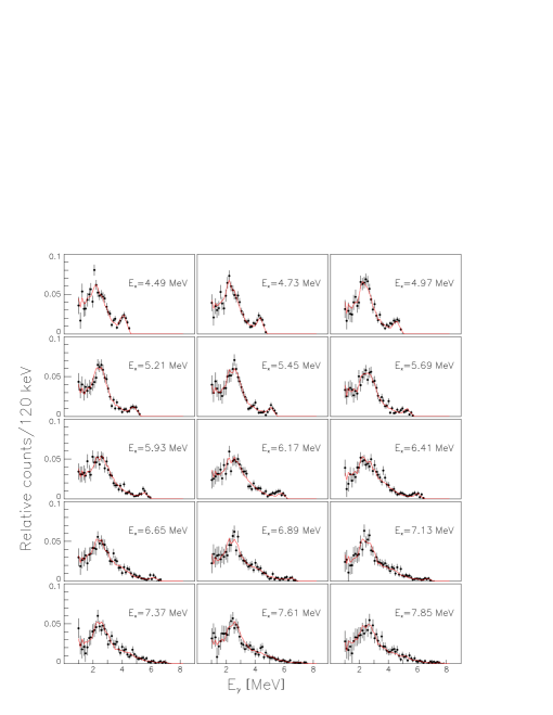
Figure 1: Normalized experimental primary $\gamma$-ray spectra with estimated errors (data points) and fit using the factorization of Eq. (1) (solid lines). The data are taken from the ¹⁶²Dy(³He,³He’)¹⁶²Dy reaction.

The primary $\gamma$-ray spectra (see Fig. 1) are the starting point of the discussion in this talk. According to the Brink-Axel hypothesis [25, 12], the primary $\gamma$-ray matrix can be factorized into two functions of one variables using

$$\Gamma(E,E_{\gamma})\propto\rho(E-E_{\gamma})\,F(E_{\gamma}),$$ (1)

where $\rho$ is the level density and $F$ is a $\gamma$-ray energy-dependent factor, proportional to the total radiative strength function i.e.

$$F(E_{\gamma})\propto\sum_{XL}E_{\gamma}^{(2L+1)}\,f_{XL}(E_{\gamma}).$$ (2)

In Eq. (1), a temperature-independent radiative strength function $f$ is assumed. Today, we know that at least the E1 strength function is temperature dependent, a fact which has already been incorporated in several models [13, 14]. However, we found for our data that the factorization according to Eq. (1) works remarkably well (see Fig. 1) which indicates that for low and slowly varying temperatures as in our case, the Brink-Axel hypothesis is approximately valid.

The details of the method to extract level density and radiative strength function from primary $\gamma$-ray spectra can be found in [8]. An extension of this method to temperature-dependent radiative strength function is discussed in Sect. 4. One detail of the method should be mentioned here. The method does not yield absolute values of the level density and the radiative strength function. Also the slope of these two functions is undetermined. Actually, all functions $\tilde{\rho}$ and $\tilde{F}$ obtained by the transformation

$$\tilde{\rho}(E-E_{\gamma}) = A\,\exp(\alpha\,[E-E_{\gamma}])\,\rho(E-E_{\gamma})$$ (3)

$$\tilde{F}(E_{\gamma}) = B\,\exp(\alpha\,E_{\gamma})\,F(E_{\gamma})$$ (4)

of any particular solution $(\rho,F)$ will fit our primary $\gamma$-ray matrix equally, since the area of the first-generation spectrum are normalized to unity for every excitation energy bin $E$, i.e.

$$\Gamma(E,E_{\gamma})=\frac{\rho(E-E_{\gamma})\,F(E_{\gamma})}{\sum_{E_{\gamma}}\rho(E-E_{\gamma})\,F(E_{\gamma})}.$$ (5)

In order to determine the parameters $A$ and $\alpha$, i.e. the absolute value and the slope of the level density, we fit our extracted level density curve to the known number of discrete levels in the vicinity of the ground state [6] and to the level density estimate obtained from neutron resonance spacing data [7] at the neutron binding energy. The only remaining free parameter then is the absolute value of the $\gamma$-ray energy-dependent factor $F$, which can be determined from the average total radiative widths of neutron capture resonances [26] by

$$\langle\Gamma_{\gamma}(E,I,\Pi)\rangle=\frac{1}{\rho(E,I,\Pi)}\sum_{XL}\sum_{I_{f},\Pi_{f}}\int_{E_{\gamma}=0}^{E}{\mathrm{d}}E_{\gamma}E_{\gamma}^{2L+1}f_{XL}(E_{\gamma})\,\rho(E-E_{\gamma},I_{f},\Pi_{f})$$ (6)

(see e.g. [27]).

In this talk, we will discuss level density and radiative strength function of ^161,162Dy and ^171,172Yb obtained from (³He,$\alpha$) reaction data and radiative strength function of ¹⁶²Dy obtained from (³He,³He’) reaction data.

3 Level density and thermodynamical quantities

Figure 2: Level density and $\gamma$-ray energy-dependent factor $F(E_{\gamma})$ of ^161,162Dy and ^171,172Yb from (³He,$\alpha$) reaction data. The error bars show the experimental uncertainties. The solid lines are extrapolations based on a shifted Fermi-gas model. The isolated points at the neutron binding energy were obtained from neutron resonance spacing data.

In Fig. 2, the nuclear level density and the $\gamma$-ray energy-dependent factor $F(E_{\gamma})$ for the nuclei ^161,162Dy and ^171,172Yb are shown. In this section, we will mainly discuss the physics of the nuclear level density. First of all, the experimental curves can be compared to popular parameterizations of the nuclear level density, like those of Gilbert and Cameron [28] or of von Egidy et al. [29]. This has been done in [30] and the conclusion is that neither of the two parameterizations can describe our data well. However, the data favor the concept of a composite level density formula as proposed in [28] with a constant-temperature level density part from above 1–2 MeV and up to approximately the neutron binding energy $B_{n}$. Another important aspect is that the experimental data of the odd and even nuclei show a relative shift in the order of the effective pairing energy $\Delta^{\mathit{eff}}(N,Z)=\Delta_{p}(N,Z)+\Delta_{n}(N,Z)-\Delta_{p}(N-1,Z)$ [30], thus the data support the concept of shifted level density formulas.

From level densities, one can easily calculate thermodynamical quantities like entropy $S$, temperature $T$, heat capacity $C_{V}$, the canonical partition function $Z$ and the average excitation energy in the canonical ensemble $\langle E\rangle$. Within the microcanonical ensemble, one obtains (in this work $k_{B}$=1)

$$S(E) = \ln\rho(E)+S_{0}$$ (7)

$$T(E) = \left(\frac{\partial S(E)}{\partial E}\right)_{V}^{-1}$$ (8)

$$C_{V}(E) = \left(\frac{\partial T(E)}{\partial E}\right)_{V}^{-1}$$ (9)

and in the canonical ensemble, one gets

$$Z(T) = \int_{0}^{\infty}N\rho(E)\exp(-E/T){\mathrm{d}}E$$ (10)

$$S(T) = \frac{\partial}{\partial T}[T\ln Z(T)]$$ (11)

$$\langle E(T)\rangle = T^{2}\frac{\partial}{\partial T}\ln Z(T)$$ (12)

$$C_{V}(T) = \left(\frac{\partial\langle E(T)\rangle}{\partial T}\right)_{V}.$$ (13)

The quantities $S_{0}$ and $N$ are necessary, since the level density is only proportional to the energy surface in the phase space $W$.

Figure 3: Caloric curve of ^161,162Dy and ^171,172Yb in the microcanonical ensemble (data points) and the canonical ensemble (line). The straight line indicates the critical temperature $T_{c}$.

In principle, one should only consider the microcanonical ensemble, since the nucleus is a closed system. However, the canonical and even the grand-canonical ensemble have often been used [1, 3] to describe thermodynamical properties of nuclei. In [31], the microcanonical and canonical entropy is discussed and compared to a simple model. One result of this discussion is that the small bumps in the experimental level density curves (see Fig. 2) can be interpreted in terms of breaking of Cooper pairs. These bumps can even be enhanced by derivating, see Eq. (8), yielding the experimental caloric curve in the microcanonical ensemble (see data points in Fig. 3 and discussion in [32]). Another important result is that the entropy excess of the odd nuclei relative to the even nuclei can be used to calculate the entropy of one quasiparticle. It is surprising that the quasiparticle entropy is constant $1.70(15)\,k_{B}$ over the whole excitation energy region investigated in [31].

When calculating the partition function in the canonical ensemble (see Eq. (10)), a strong smoothing is introduced due to the Laplace transformation involved. It is also worth noting that in order to calculate thermodynamical quantities reliably up to $T\sim 1$ MeV, one has to know the level density up to $\sim 40$ MeV. Since the experimental level density curves are only known up close to the neutron binding energy, they had to be extrapolated by a model. We have chosen the shifted Fermi-gas parameterization of von Egidy et al. [29] multiplied by a constant factor in order to match the neutron resonance spacing data.

Figure 4: Semi-experimental heat capacity as function of temperature in the canonical ensemble for ^161,162Dy and ^171,172Yb. The dashed lines describe the approximate Fermi-gas heat capacity. The arrows indicate the first local maxima of the experimental curve relative to the Fermi-gas estimates. The dashed-dotted lines describe estimates according to a constant-temperature level density formula, where $T$ is set equal to the critical temperature $T_{c}$ (vertical lines).

Due to this strong smoothing over a huge range of excitation energies, one does not expect to see fine structures in the canonical ensemble. This is clearly demonstrated in Fig. 3, where the canonical caloric curve is smooth and the breaking of individual Cooper pairs is completely washed out. However, the quenching of pairing correlations is manifested in the canonical heat-capacity curves (see Fig. 4). Deviating from a Fermi-gas estimate, the heat-capacity curves show pronounced S-shapes with local maxima relative to the smooth Fermi-gas estimate. This behavior can be explained by the fact that the level density exhibits a constant-temperature part at low excitation energies. Therefore the canonical heat capacity curve $C_{V}=(1-T/\tau)^{-2}$ for a constant-temperature level density $\rho=C\exp(E/\tau)$ has been fitted to the data at low temperatures, and the parameter $\tau$ is interpreted as the critical temperature for the quenching of pairing correlations [33]. The resulting critical temperatures are given as horizontal and vertical lines in Figs. 3 and 4 respectively. We interpret the S-shape of the heat capacity as a fingerprint of a second-order phase-transition-like phenomenon in finite systems, where the transition goes from a phase with strong pairing correlations (usually referred to as a superfluid phase) to a phase with weak pairing correlations (normal fluid phase). This phase-transition-like phenomenon has been anticipated by many theoretical works [2, 4, 34, 35].

4 Radiative strength function

Figure 5: Radiative strength function of ^161,162Dy and ^171,172Yb (data points). The absolute normalization of the data is still preliminary. The error bars show the experimental uncertainties only. The solid lines are strength function models (see text) where all parameters are taken from other experimental systematics and nothing was fitted to our data beside $k\sigma_{p}$ (see text).

Fig. 5 shows the radiative strength functions of ^161,162Dy and ^171,172Yb compared to model calculations. For the theoretical calculation, we have used the E1 model of Sirotkin [14], where we take the expression for the temperature-dependent width of Kadmenskiĭ et al. [13]. The parameters are taken from an interpolation of the experimental systematics of [17]. The temperature has been assumed as constant with $T\sim 500$ keV. For the M1 model we simply take a Lorentzian, where the parameters for the centroids and widths are taken from [27] and the parameters for the resonance strengths are taken from $f_{M1}/f_{E1}$ systematics [36], evaluated at $E_{\gamma}=B_{n}-1$ MeV. For the pygmy resonance, we use again a Lorentzian with parameters from an interpolation based on the experimental systematics [18]. It is amazing that the model calculation can fit our data so well. Both, the absolute value as well as the slope of the experimental strength functions could be reproduced without fitting any parameter from the models except $k\sigma_{p}$. Here we had to reduce the parameters for the pygmy resonance strength $k\sigma_{p}$ by 30–70% as the only compromise to our data.

In the following, we want to investigate the strength of the pygmy resonance, which is the only parameter we had to fit in order to describe our data. For this reason, we divide our primary $\gamma$-ray matrix into four subsets of distinct excitation energy bins. Each excitation energy bin is 1 MeV broad, thus we can assume that the nuclear temperature within every excitation energy bin is constant and the Brink-Axel hypothesis remains valid. However, for the different excitation energy bins the nuclear temperature is in general different. We extract radiative strength functions from those four excitation energy bins. In that way we obtain radiative strength functions for four different nuclear temperatures. This provides an easy way to investigate the temperature dependence of the radiative strength function.

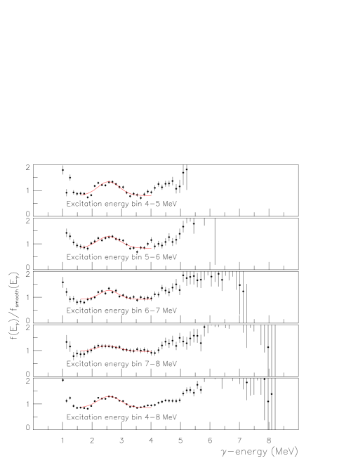
Figure 6: Relative radiative strength functions extracted from different excitation energy bins. The data here and in the following discussion are from the ¹⁶²Dy(³He,³He’)¹⁶²Dy reaction. The radiative strength functions are all divided by the same smooth strength function $CE_{\gamma}^{n}$ with $n\approx 1.2$ in order to enhance the pygmy resonance structure.

Figure 7: Fit parameters from a Gaussian fit to the pygmy resonance structure (see Fig. 6 for different excitation energy bins. The centroid and the width are constant and fit nicely into the systematics of Ref. [18]. The relative strength is decreasing with increasing excitation energy. The lines indicate average values, taking into account the whole data set.

Figure 8: Temperature dependence of the relative pygmy resonance strength.

In Fig. 6, the relative radiative strength functions from the different excitation energy bins are plotted. One can see immediately that the pygmy resonance strength is highly temperature dependent. On the other hand, the general slope of the radiative strength function is constant, thus the gross features of the strength function are rather independent of nuclear temperature, justifying the use of the Brink-Axel hypothesis for our data analysis. The fit parameters of the pygmy resonance for the different excitation energy bins are shown in Fig. 7. Obviously, only the resonance strength of the pygmy resonance shows a pronounced temperature dependence, whereas the centroid and the width are nearly independent of temperature. The temperature dependence becomes even much more obvious when we actually translate the excitation energy bins into nuclear temperature using the canonical caloric curve of Fig. 3. The result is given in Fig. 8, where the temperature dependence of the pygmy resonance strength is shown. A clear quenching of the pygmy resonance strength as function of temperature is observed.

We have to speculate on the physical origin of the observed quenching. In the first place, it is not at all clear if the pygmy resonance is a phenomenon in the electric or magnetic dipole strength function. Igashira et al. [18] favor electric dipole strength without measuring the parity of the transition, whereas in other works, spin-flip [37] or orbital [38] (scissors mode) M1 strength has been proposed. Anyhow, we might assume a strong dependence of the pygmy resonance strength on the deformation parameter $\delta$ (like it is observed for the scissors mode [39]). A quenching of the pygmy resonance strength would then correspond to a shape transition of the nucleus from deformed to spherical. This temperature-induced shape transition was indeed anticipated for ¹⁷⁰Dy in [3] at temperatures around 500 keV. Therefore, we speculatively interpret the quenching of the pygmy resonance strength as a fingerprint for a temperature-induced shape transition.

5 Conclusion

A method to extract simultaneously level density and radiative strength function from primary $\gamma$-ray spectra without assuming any model for either of them has been presented. Thermodynamical quantities have been deduced within the microcanonical and the canonical ensemble. We observe structures in these quantities which can be interpreted as breaking of Cooper pairs and quenching of pairing correlations and we observe a fingerprint of the phase-transition-like phenomenon from a superfluid-like phase to a normal-fluid-like phase. Further on, the critical temperature of this transition has been determined. We are able to reproduce our experimental strength functions by the use of models, where all parameters except the pygmy resonance strength are taken from other experimental systematics. The temperature dependence of the pygmy resonance strength has been investigated and a significant quenching around $T\approx 500$ keV has been observed, which we interpret tentatively as the result of a temperature-induced shape transition.

6 Acknowledgments

The authors are grateful to E. A. Olsen and J. Wikne for providing the excellent experimental conditions. We thank A. Voinov for many interesting discussions. We wish to acknowledge the support from the Norwegian Research Council (NFR).

References

- [1] H. A. Bethe, Phys. Rev. 50, 332 (1936).
- [2] M. Sano, and S. Yamasaki, Prog. Theor. Phys. 29, 397 (1963).
- [3] S. E. Koonin, D. J. Dean, and K. Langanke, Phys. Rep. 278, 1 (1997).
- [4] H. Nakada, and Y. Alhassid, Phys. Rev. Lett. 79, 2939 (1997).
- [5] J. A. White, S. E. Koonin, and D. J. Dean, Phys. Rev. C 61, 034303 (2000).
- [6] R. B. Firestone, and V. S. Shirley, Table of Isotopes, edition, Vol. II (New York: John Wiley & Sons, Inc., 1996).
- [7] A. S. Iljinov, M. V. Mebel, N. Bianchi, E. De Sanctis, C. Guaraldo, V. Lucherini, V. Muccifora, E. Polli, A. R. Reolon, and P. Rossi, Nucl. Phys. A543, 517 (1992).
- [8] A. Schiller, L. Bergholt, M. Guttormsen, E. Melby, J. Rekstad, and S. Siem, Nucl. Instrum. Methods Phys. Res. A 447, 498 (2000).
- [9] W. Hauser, and H. Feshbach, Phys. Rev. 87, 366 (1952).
- [10] Thomas Rauscher, Friedrich-Karl Thielemann, and Karl-Ludwig Kratz, Phys. Rev. C 56, 1613 (1997).
- [11] V. Weisskopf, Phys. Rev. 83, 1073 (1951).
- [12] P. Axel, Phys. Rev. 126, 671 (1962).
- [13] S. G. Kadmenskiĭ, V. P. Markushev, and V. I. Furman, Yad. Fiz. 37, 277 (1983) [Sov. J. Nucl. Phys. 37, 165 (1983)].
- [14] V. K. Sirotkin, Yad. Fiz. 43, 570 (1986) [Sov. J. Nucl. Phys. 43, 362 (1986)].
- [15] V. G. Soloviev, A. V. Sushkov, N. Yu. Shirikova, and N. Lo Iudice, Nucl. Phys. A613, 45 (1997).
- [16] V. G. Soloviev, A. V. Sushkov, and N. Yu. Shirikova, Phys. Rev. C 56, 2528 (1997).
- [17] G. M. Gurevich, L. E. Lazareva, V. M. Mazur, S. Yu. Merkulov, G. V. Solodukhov, and V. A. Tyutin, Nucl. Phys. A351, 257 (1981).
- [18] M. Igashira, H. Kitazawa, M. Shimizu, H. Komano, and N. Yamamuro, Nucl. Phys. A457, 301 (1986).
- [19] F. Bečvář, P. Cejnar, J. Honzátko, K. Konečný, I. Tomandl, and R. E. Chrien, Phys. Rev. C 52, 1278 (1997).
- [20] S. Goriely, Talk at the ECT∗ Workshop on ’Advances in Shell-Model Studies in Nuclei far from Stability’, Trento (Italy), 14-25 June 1999.
- [21] M. Guttormsen, A. Atac, G. Løvhøiden, S. Messelt, T. Ramsøy, J. Rekstad, T. F. Thorsteinsen, T. S. Tveter, and Z. Zelazny, Phys. Scr. T32, 54 (1990).
- [22] M. Guttormsen, T. S. Tveter, L. Bergholt, F. Ingebretsen, and J. Rekstad, Nucl. Instrum. Methods Phys. Res. A 374, 371 (1996).
- [23] M. Guttormsen, T. Ramsøy, and J. Rekstad, Nucl. Instrum. Methods Phys. Res. A 255, 518 (1987).
- [24] A. Schiller, M. Guttormsen, E. Melby, J. Rekstad, and S. Siem, Phys. Rev. C 61, 044324 (2000).
- [25] D. M. Brink, Ph.D. thesis, Oxford University, 1955.
- [26] S. F. Mughabghab, Neutron cross sections, Vol. 1, Part B (New York: Academic Press, 1984).
- [27] J. Kopecky and M. Uhl, Phys. Rev. C 41, 1941 (1990).
- [28] A. Gilbert and A. G. W. Cameron, Can. J. Phys. 43, 1446 (1965).
- [29] T. von Egidy, H. H. Schmidt, and A. N. Behkami, Nucl. Phys. A481, 189 (1987).
- [30] M. Guttormsen, M. Hjorth-Jensen, E. Melby, J. Rekstad, A. Schiller, and S. Siem, Phys. Rev. C 61, 067302 (2000).
- [31] M. Guttormsen, A. Bjerve, M. Hjorth-Jensen, E. Melby, J. Rekstad, A. Schiller, S. Siem, and A. Belic, Phys. Rev. C 62, 024306 (2000).
- [32] E. Melby, L. Bergholt, M. Guttormsen, M. Hjorth-Jensen, F. Ingebretsen, S. Messelt, J. Rekstad, A. Schiller, S. Siem, and S. W. Ødegård, Phys. Rev. Lett. 83, 3150 (1999).
- [33] A. Schiller, A. Bjerve, M. Guttormsen, M. Hjorth-Jensen, F. Ingebretsen, E. Melby, S. Messelt, J. Rekstad, S. Siem, and S. W. Ødegård, Preprint nucl-ex/9909011 (http://xxx.lanl.gov/).
- [34] D. J. Dean, S. E: Koonin, K. Langanke, P. B. Radha, and Y. Alhassid, Phys. Rev. Lett. 74, 2909 (1995).
- [35] S. Rombouts, K. Heyde, and N. Jachowicz, Phys. Rev. C 58, 3295 (1998).
- [36] J. Kopecky and M. Uhl, in Proceedings of a Specialists’ Meeting on Measurement, Calculation and Evaluation of Photon Production Data, Bologna, Italy 1994 (NEA/NSC/DOC(95)1) p. 119.
- [37] M. Guttormsen, J. Rekstad, A. Henriquez, F. Ingebretsen, and T. F. Thorsteinsen, Phys. Rev. Lett. 52, 102 (1984).
- [38] C. Wesselborg, P. von Brentano, K. O. Zell, R. D. Heil, H. H. Pitz, U. E. P. Berg, U. Kneissl, S. Lindenstruth, U. Seeman, and R. Stock , Phys. Lett. B 207, 22 (1988).
- [39] N. Pietralla, P. von Brentano, R.-D. Herzberg, U. Kneissl, N. Lo Iudice, H. Maser, H. H. Pitz, and A. Zilges, Phys. Rev. C 58, 184 (1998).