New Limit on the $D$ Coefficient in Polarized Neutron Decay

Abstract

We describe an experiment that has set new limits on the time reversal invariance violating $D$ coefficient in neutron beta-decay. The emiT experiment measured the angular correlation $\langle\mathbf{J}\rangle\cdot({\mathbf{p}}_{e}\times{\mathbf{p}}_{p})$ using an octagonal symmetry that optimizes electron-proton coincidence rates. The result is $D=[-0.6\pm 1.2({\rm stat})\pm 0.5({\rm syst})]\times 10^{-3}$. This improves constraints on the phase of $g_{A}/g_{V}$ and limits contributions to $T$ violation due to leptoquarks. This paper presents details of the experiment, data analysis, and the investigation of systematic effects.

]

I Introduction

$CP$ violation has been observed so far only in the decays of neutral kaons [1]. Recently evidence for the implied $T$ violation in the neutral kaon system has been reported [2]. These effects could be due to the Kobayashi-Maskawa phase in the Standard Model [3]. However, these observations could also be due to new physics, and it is well-established that new sources of $CP$ violation are required by the observed baryon asymmetry of the universe [4]. Many extensions of the Standard Model contain new sources of $CP$ violation and can be probed in observables for which the contribution of the Kobayashi-Maskawa phase in the Standard Model is small. The present experiment searches for $CP$ violation in one such observable, a $T$-odd correlation in the decay of free neutrons.

The differential decay rate for a free neutron can be written [5]

$$dW\propto S(E_{e})dE_{e}d\Omega_{e}d\Omega_{\nu}\left[1+a\frac{\mathbf{p}_{e}\cdot\mathbf{p}_{\nu}}{E_{e}E_{\nu}}\right.$$ (1)

$$\left.+\frac{\langle\mathbf{J}\rangle}{J}\cdot\left(A\frac{\mathbf{p}_{e}}{E_{e}}+B\frac{\mathbf{p}_{\nu}}{E_{\nu}}+D\frac{\mathbf{p}_{e}\times\mathbf{p}_{\nu}}{E_{e}E_{\nu}}\right)\right],$$ (2)

where $p_{e}$, $E_{e}$ and $p_{\nu}$, $E_{\nu}$ are the momentum and energy of the outgoing electron and neutrino, respectively, $S(E_{e})$ is a phase space factor, and $\langle\mathbf{J}\rangle$ is the neutron spin. The triple-correlation $D\langle\mathbf{J}\rangle\cdot(\mathbf{p}_{e}\times\mathbf{p}_{\nu})$ is odd under motion reversal, and can be used to measure time reversal invariance violation when final state interactions are taken into account. Note that in the rest frame of the neutron, conservation of momentum allows the transformation of the triple-correlation term into

$$-D\frac{\langle\mathbf{J}\rangle}{J}\cdot\frac{\mathbf{p}_{e}\times\mathbf{p}_{p}}{E_{e}E_{\nu}}$$

where $\mathbf{p}_{p}$ is the momentum of the recoil proton.

The $D$ coefficient is sensitive only to $T$-odd interactions with vector and axial vector currents. In a theory with such currents, the coefficients of the correlations depend on the magnitude and phase of $\lambda=|\lambda|e^{-i\phi}$, where $|\lambda|=|g_{A}/g_{V}|$ is the magnitude the ratio of the axial vector to vector form factors of the nucleon. In this notation, the coefficients are given by

$$a=\frac{1-|\lambda|^{2}}{1+3|\lambda|^{2}},\quad A=-2\frac{|\lambda|\cos\phi+|\lambda|^{2}}{1+3|\lambda|^{2}},$$ (3)

$$B=-2\frac{|\lambda|\cos\phi-|\lambda|^{2}}{1+3|\lambda|^{2}},\quad D=2\frac{|\lambda|\sin\phi}{1+3|\lambda|^{2}}.$$ (4)

The most accurate determinations of $|\lambda|$ (current world average $|\lambda|=1.2670\pm 0.0035)$ come from measurements of $A$ [6]. The coefficients $a$, $A$, and $B$, respectively, are measured to be $-0.102\pm 0.005$, $-0.1162\pm 0.0013$, and $0.983\pm 0.004$ [6]. Several previous experiments found the value of $D$, and thus $\sin\phi$, to be consistent with zero at a level of precision well below 1%. The three most recent such measurements found $D=(-1.1\pm 1.7)\times 10^{-3}$ [7] and $D=(2.2\pm 3.0)\times 10^{-3}$ [8], and $D=(-2.7\pm 5.0)\times 10^{-3}$ [9], constraining $\phi$ to $180.07^{\circ}\pm 0.18^{\circ}$ [6].

Final state interactions give rise to phase shifts of the outgoing electron and proton Coulomb waves that are time reversal invariant but motion reversal non-invariant. Thus $D$ has terms that arise from phase shifts due to pure Coulomb and weak magnetism scattering. The Coulomb term vanishes in lowest order in V-A theory [5], but scalar and tensor interactions could contribute. The Fierz interference coefficient measurements [10, 11] can be used in limiting this possible contribution to

$$|D^{EM}|<(2.8\times 10^{-5})\frac{m_{e}}{p_{e}}.$$ (5)

Interference between Coloumb scattering amplitudes and the weak magnetism amplitudes produces a final state effect of order (${{E_{e}}^{2}}/{p_{e}m_{n}}$). This weak magnetism effect is predicted to be [12]

$$D^{WM}=1.1\times 10^{-5}.$$ (6)

The $D$ coefficient has also been measured for ¹⁹Ne decay, with the most precise experiment finding $D_{Ne}=(4\pm 8)\times 10^{-4}$ [13]. The predicted final state effects for ¹⁹Ne are approximately an order of magnitude larger than those for the neutron and may be measured in the next generation of ¹⁹Ne experiments. For ⁸Li, a triple-correlation of nuclear spin, electron spin and electron momentum has been measured, with the most precise measurement at $R=(0.9\pm 2.2)\times 10^{-3}$ [14]. Unlike $D$, a nonzero $R$ requires the presence of scalar or tensor couplings and thus is a tool to search for such couplings. The electric dipole moments (EDMs) of the electron [15], neutron [16], and ¹⁹⁹Hg atom [17] are arguably the most precisely-measured $T$-violating parameters and bear on many of the same theories as $D$. Table I summarizes the current constraints on $D$ from analyses of data on other $T$-odd observables for the Standard Model and extensions [18]. For lines 2-5 these limits are derived from the measured neutron or ¹⁹⁹Hg EDM.

Theory	$D$
1. Kobayashi-Maskawa Phase	$<10^{-12}$
2. Theta-QCD	$<10^{-14}$
3. Supersymmetry	$\lesssim 10^{-7}-10^{-6}$
4. Left-Right Symmetry	$\lesssim 10^{-5}-10^{-4}$
5. Exotic Fermion	$\lesssim 10^{-5}-10^{-4}$
6. Leptoquark	$\leq$present limit

TABLE I.: Constraints on $D$ from analyses of other $T$-odd observables for the Standard Model and extensions.

In the nearly two orders of magnitude between the present limit on $D$ and the final state effects lies the opportunity to directly observe or limit new physics. Moreover, accurate calculations of magnitude and energy dependence of the final state effects can be made to extend the range of exploration still further.

II Overview of the emiT Detector

In the emiT apparatus, a beam of cold neutrons is polarized and collimated before it passes through a detection chamber with electron and proton detectors (four each). A schematic of the experiment is shown in Figure 1.

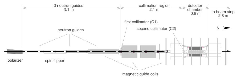
FIG. 1.: The emiT experimental apparatus beamline layout. The neutrons traveled through 8.8 meters of guides and vacuum components before reaching the beam stop.

The most significant improvements over previous experiments are the achievement of near-unity polarization ($>93\%$ compared to 70% in [7]) and the construction of a detector with greater acceptance and greater sensitivity to the $D$ coefficient. The octagonal arrangement of the eight detector segments gives them nearly full coverage of the 2$\pi$ of azimuthal angle around the beam, nearly twice the angular acceptance in previous experiments, and the detector segments are longer than in previous experiments. The placement of the two types of detectors at relative angles of 135^∘ is also an improvement over previous experiments, in which the coincidences were detected at 90^∘. While the cross product is greatest at 90^∘, the preference for larger electron-proton angles in the decay makes placement of the detectors at 135^∘ the best choice to achieve greater symmetry, greater acceptance, and greater sensitivity to $D$ (see Figure 2).

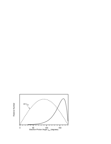
FIG. 2.: Although the cross-product (dashed line) is maximized at electron-proton detection angles of 90^∘, the overall sensitivity to $D$ (solid line) is enhanced at larger angles due to the phase space for the decay. Placing the detectors at 135^∘ allows for an octagonal geometry that combines greater symmetry, acceptance, and sensitivity when compared to placement of the detectors at 90^∘. The solid curve in this figure is the sensitivity for a zero-radius beam, which would exhibit a factor of 7 enhancement for 135^∘ as compared to 90^∘. For our nearly 3 cm-radius beam, the enhancement factor is close to 3.

Combined with the higher neutron polarization from the supermirror polarizer our geometry provides for an overall sensitivity to $D$ that is a factor of $\approx 7$ greater than previous measurements, assuming the same cold neutron beam flux.

The first run of the experiment was conducted at the NIST Center for Neutron Research (NCNR) in Gaithersburg, MD. The experimental apparatus is outlined below, while more detailed descriptions can be found in [19, 20].

A Polarized Neutron Beam

The NCNR operates a 20-MW, heavy-water-moderated research reactor. Neutrons from the reactor pass through a liquid hydrogen moderator to make cold neutrons with an approximately Maxwellian velocity distribution at a temperature of about 40 K. The average neutron velocity is about 800 m/s. The neutrons are transported 68 meters to the apparatus via a ⁵⁸Ni-lined neutron guide. Neutrons are totally internally reflected if they enter with an angle of incidence less than 2 mrad for each Å of de Broglie wavelength. The capture flux of the neutrons was measured using a gold foil activation technique to be $\rho_{n}v_{0}=1.4\times 10^{9}$n/cm²/s (where $v_{0}$ = 2200 m/s) at the end of the neutron guide. (The capture flux quantifies the neutron density in the detector for the polychromatic beam.) The beam passes through a cryogenic beam filter of 10-15 cm of single crystal bismuth which filters out residual fast neutrons and gamma-rays.

The neutrons are polarized with a double-sided bender-type supermirror polarizer obtained from the Institut Laue-Langevin in Grenoble, France [21]. The supermirror consists of 40 Pyrex [22] plates coated on both sides with cobalt, titanium, and gadolinium layers that maximize the reflection of neutrons with the desired spin state while absorbing nearly all neutrons of the opposite spin state. The supermirror was measured to polarize a 4.5 cm by 5.5 cm beam with 24% transmission relative to the incident unpolarized flux. The neutron polarization was determined to be $>93\%$ ($95\%$ CL).

The neutrons travel the one meter from the polarizer to the spin-flipper inside a Be-coated glass flight tube in which a small helium overpressure is maintained to minimize beam attenuation via air scattering. The neutrons, which have spins that are transverse to their motion, then pass through two layers of aluminum wires which comprise the current-sheet spin flipper. When the current in the second layer is antiparallel to that in the first there is no net magnetic field and the neutron polarization is unaffected. When the currents are parallel, the neutron spin does not adiabatically follow the rapid change in field orientation and thus the sense of $\langle\mathbf{J}\rangle\cdot\mathbf{B}$ is reversed. Downstream of the spin flipper, weak magnetic fields adiabatically rotate the spin to longitudinal, i.e. parallel or antiparallel to the neutron momentum. The longitudinal guide fields are 2.5 mT upstream and 0.5 mT within the detector. Figure 3 shows the spin transport system. The polarization direction is reversed every 5 seconds.

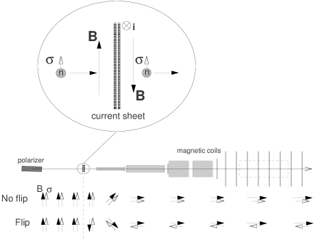
FIG. 3.: Two sheets of current-carrying wires create a magnetic field of opposite orientation on each side. The field orientation changes so rapidly that the spin of a neutron passing through the current sheets cannot follow the field reversal, and the neutron polarization is reversed with respect to the magnetic guide field. Downstream the magnetic field and polarization are rotated adiabatically from transverse in orientation to longitudinal.

In the detection region, the longitudinal field is produced by eight 50 amp-turn current loops of 1 m diameter. The loops are aligned to within 10 mrad of the detector axis using a sensitive field probe and an AC lock technique. Additional coils canceled the transverse components of the Earth’s field and local gradients of 7.5 $\mu$T/m.

The vacuum chamber begins at the spin flipper with two meters of Be-coated flight tubes, through which the neutrons travel toward the collimator region. Two collimators of 6 cm and 5 cm diameter openings separated by 2 m define the beam. These and 5 additional “scrapers” between them consist of rings of ⁶LiF which absorb the neutrons. Behind each ring is a thick ring of high-purity lead which absorbs the gamma-rays from the reactor and those produced by neutron captures upstream. Between scrapers, the walls of the beam tube are lined with ⁶Li-loaded glass to absorb stray neutrons.

A fission chamber mounted behind a sheet of ⁶Li-glass with a 1 mm pinhole aperture was scanned across the beam to obtain a cross-sectional profile of the intensity as shown in Figure 4. The neutron intensity was measured before and after the experiment. To determine the polarization at the entrance to the detector, the beam passed through a second, single-sided, analyzing supermirror directly in front of the scanning detector, and the ratio of intensities with the spin flipped and unflipped was measured. The resulting flippng ratio measures a combination of the neutron-spin-dependent transmission efficiencies of the two supermirrors and the neutron spin flipping eficiency. From this, and assumptions about the spin flipping efficiency, we can determine the product of polarization efficiencies for the two supermirrors (polarizer and analyzer). When the upper limit of 100% spin flipping efficiency is used, a lower limit of the neutron beam polarization of $93\%$ ($95\%$ CL) is found. This lower limit also includes the assumption that the flipping ratio for a pair of supermirrors identical to our analyzer would be less than that of a pair of supermirrors identical to our polarizer by a factor of $2\pm 0.5\%$[21].

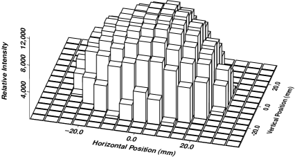
FIG. 4.: Neutron beam intensity profile at the entrance to the detection region obtained from a scan across the beam face.

Downstream of the detection region the vacuum chamber diameter increases to 40.6 cm, terminating with a ⁶Li-glass beam stop 2.8 m from the end of the detector. A 1 mm diameter pinhole at the center of the beamstop allows about 1% of the beam to pass through a silicon window into a fission chamber detector that continuously monitors the neutron flux.

B Detector System

Eight detectors surround the beam, each 10 cm from the beam axis as shown in Figure 5. The octagonal geometry places electron and proton detectors at relative angles of 45 and 135 degrees. Coincidences are counted between detectors at relative angles of 135 degrees.

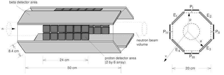
FIG. 5.: Basic detector geometry - an octagonal array of four each proton and electron detectors.

1 Electron Detectors

The electron detectors are slabs (8.4 cm x 50 cm x 0.64 cm) of BC408 plastic scintillator connected on each end to curved lucite light-guides that channel the light to Burle 8850 photomultiplier tubes. Each photomultiplier tube is surrounded by a mu-metal magnetic shield and a pair of nested solenoids acting as an active magnetic shield. This combination of active and passive magnetic shielding had a factor of 10 less impact (0.5 $\mu$T) on the guide field at the beam center than the mu-metal alone.

The scintillator thickness of 0.64 cm is just greater than that necessary to stop the most energetic (782 keV) of the electrons from neutron. The scintillators are wrapped with aluminized mylar and aluminum foil to prevent charging and to shield the detectors from x-rays and field-emission electrons in the vacuum chamber. For each segment, the energy response was calibrated with cosmic-ray muons and conversion electrons from ²⁰⁷Bi and ¹¹³Sn (see Figure 6.)

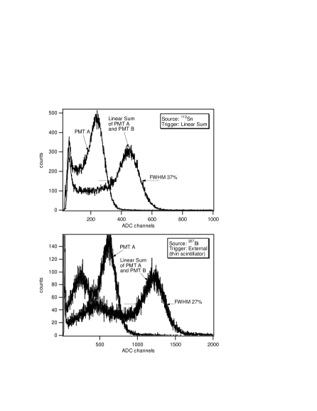
FIG. 6.: Spectra produced during the energy calibration of the electron detectors. Shown are histograms of the charge collected in an individual phototube (PMT A) and of the total charge in the analog hardware sum of the two phototube signal. The spectrum in PMT B (not shown) is roughly identical to that in PMT A. For the ¹¹³Sn, a level-crossing discriminator triggers on the analog sum signal. The peak visible is the 364 keV conversion electron. To suppress the contribution of gamma-rays in the ²⁰⁷Bi spectra the data acquisition is triggered on a thin scintillator placed between the source and the detector. The largest feature in these spectra falls at an energy of 882 keV (the 976 keV conversion electron energy minus the energy loss in the thin scintillator.)

2 Proton Detectors

Each proton detector has an array of 12 PIN diodes of 500 micrometer thickness arranged in two rows of 6. The diodes are held within a stainless steel high voltage electrode. Over each diode an open cylinder protrudes from the face of the electrode, shaping the field to focus and accelerate the protons as shown in Figure 7. Thus each diode collects protons focused from a region 4 cm $\times$ 4 cm even though it has an active area of only 1.8 cm $\times$ 1.8 cm.

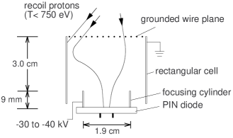
FIG. 7.: Geometry of the electrodes that accelerate and focus the protons onto a PIN diode.

The diodes and their electronics are held at -30 to -40 kV. Between the electrode and the beam is a frame strung with 80 0.08-mm gold-plated tungsten wires that define a plane of electrical ground. Protons drift in a field-free region until they pass this plane, and then are accelerated by the high voltage and focused onto the nearest PIN diode below. Near both ends of the detector array are two cryopanels held at liquid nitrogen temperature. Water vapor, released predominantly by the scintillators and other plastic components, is pumped onto the cryopanels to prevent condensation on the cooled PIN diodes.

The charge in the PIN diode produced by each proton is amplified by 10 V/pC with a preamplifier mounted directly behind the PIN diode. These circuits and the PIN diodes are cooled with liquid nitrogen to about 0^∘C to decrease electronic noise. Preamplifier signals are processed in a custom VME-format shaper/ADC board with programmable gain and operating mode parameters. The PIN diodes were calibrated with x-rays from an ²⁴¹Am source as shown in Figure 8.

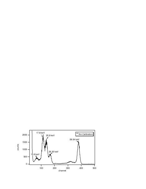
FIG. 8.: Energy calibration spectrum of a PIN diode detector using an ²⁴¹Am source. The FWHM is 2.9 keV at the 59.5 keV line.

3 Background

The background in the detectors was primarily related to the beam or to the high voltage bias. Closing the beam shutter upstream of the neutron filter stops virtually all neutrons and about 1/3 of the gamma-rays coming from the reactor along the beamline. With the shutter closed, the rates in each detector were less than 100 Hz, primarily from dark current, reactor gamma-rays, and cosmic rays. With the shutter open, the detectors see an increased gamma-ray flux primarily from neutron captures in the apparatus, triggering the detectors at less than 1 kHz per electron detector and less than 1 kHz for all PIN diodes combined. This results in deadtime less than 3% for the beam-related background. At its worst, the high-voltage-related background, consisting of x-rays, light, electrons, and ions, led to rates in the hundreds of kHz in the detectors. It was reduced at times by conditioning and cleaning of electrodes but varied by orders of magnitude during the run.

C Data Acquisition

A block diagram of the data acquisition system is shown in Figure 9. The identification of neutron decay events is simplified by the fact that the proton signal is observed 0.5 $\mu$s to 2 $\mu$s after the electron signal. The recoil protons, with maximum energies of only 750 eV, require this time to drift from the point of decay to the face of the proton detector. Events are accepted by the coincidence trigger when the electron signal arrives within a coincidence time window $\pm\tau_{coinc}/2$ of a proton signal. The duration $\tau_{coinc}$ of this window was originally 14 $\mu$s and was shortened to 7 $\mu$s midway through the experiment to reduce the system deadtime. Each stored event contains the location (PIN diode) and energy for the proton event, location (electron detector), energy of the electron event, relative time between individual signals from the two phototubes in the electron detector, relative time of arrival of the proton and electron signals, and the orientation of the neutron polarization. Every 30 seconds during the data collection, information is recorded from the system monitors which include system livetime, magnet currents, neutron flux at the beam stop, vacuum pressure, proton detector high voltage, and high voltage leakage current. Periodically, the data acquisition collects singles spectra from all of the individual detectors.

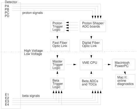
FIG. 9.: Data acquisition components.

III Experimental Run

A Data Collection

The experiment was installed at the NCNR during December 1996 and January 1997. From February through August 1997, 50 GB of data were collected and stored. The data are divided into 626 files representing continuous runs, typically four hours in duration. These are grouped into 125 series, within which running conditions varied little. For one week in August a systematic test was run in which the beam was distorted and the polarization guide field direction changed. The purpose and results of this test will be described in Section IV.

Instabilities in the proton detector high voltage made it impossible to operate all channels of the detectors at all times. Sometimes the electrodes simply would not hold the necessary voltage, and at other times a large spark or series of sparks would damage the electronics held at high voltage. Less than half of the data were collected when all four proton detectors were functioning. Another limitation to the detector uniformity were variations in the measured proton energy deposited in the PIN diodes. In preliminary tests, the surface dead-layers of the PINs were measured to be 20$\pm 2$ $\mu$g/cm² as specified by the manufacturer, Hamamatsu. In a dead-layer of this thickness a 35 keV proton loses 10 keV of energy. The proton energies measured during the experiment, however, were 12-18 keV, an average of 20 keV below the energy imparted to them by acceleration through 34-38 kV (see Figure 10.) With widths (FWHM) of approximately 10 keV, these peaks are not well separated from the background.

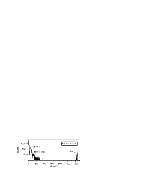
FIG. 10.: Energy spectrum in PIN diode III14, near which is mounted a weak ¹¹⁹Sn source producing a 24 keV x-ray. The protons, accelerated to 36 keV but measured at less than 20 keV, are visible between the background and the x-ray peak. The peak on the far right from a low-rate pulser input directly into the preamplifier is used to monitor gain and resolution.

High background rates necessitated the setting of thresholds at levels such that some neutron decay events were also rejected. This and the data acquisition deadtime were the primary limitations to the statistics of the experiment. A deadtime per event of 2 ms was necessary for stability of the system. Even with the reduction in length of the coincidence window, the high rate of background kept the system at 40-60% deadtime for most of the data collection period.

B Event Selection

Figure 11 shows an example of the relative time spectrum for the coincidence data. The large center spike, originating mainly from multiple gamma rays produced by neutron captures in the apparatus, defines zero time difference. The neutron decay events are accepted within a window 0.35 $\mu$s to 0.9 $\mu$s after the prompt peak. This window contains the majority of the neutron decay protons, while excluding the tail of the prompt peak and the low-signal-to-background tail of the proton peak. The background to be subtracted from these events is estimated using the rates in regions to either side of the decay and zero-time peaks.

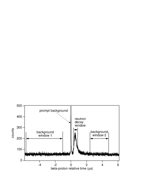
FIG. 11.: Time windows used to find the signal and estimate the background.

Events are also selected on the basis of measured proton energy to reduce the amount of background to be subtracted. The energy range accepted is chosen solely by minimizing the fractional statistical uncertainty in the number of neutron decay events for each PIN diode-electron detector pair. Specifically, if $N_{\Delta}$ is the number of coincidences counted by subtracting the background from the coincidences in the 0.35 to 0.9 $\mu$s window, the energy range is chosen to minimize

$$\frac{\sigma_{N_{\Delta}}}{N_{\Delta}}\approx\frac{\sqrt{1+1/f}}{\sqrt{N_{\Delta}}},$$ (7)

where $f$ is the signal to background ratio in this energy range. This increases the overall signal to background on the 15 million good events from 0.8 to 2.5.

IV Data Analysis and Uncertainty Estimation

A Determination of $D$ from Coincidence Events

For each PIN diode-electron detector pair in a given data series, the count rate can be expressed as

$$N_{\pm}^{\alpha i}=N_{0}\epsilon^{\alpha}\epsilon^{i}\big{[}K^{\alpha i}_{1}+aK^{\alpha i}_{a}\pm P{\hat{\sigma}}\cdot$$ (8)

$$(A{\mathbf{K}}^{\alpha i}_{A}+B{\mathbf{K}}^{\alpha i}_{B}+D{\mathbf{K}}^{\alpha i}_{D})\big{]},$$ (9)

where $N_{0}$ is a constant proportional to the beam flux, the $\epsilon^{\alpha}$ and $\epsilon^{i}$ are detector efficiencies for a PIN diode and electron detector respectively. The average of the neutron polarization vector over the detector volume, given by $P\hat{\sigma}$,is assumed to be uniform and constant over time, lying along the direction of the 0.5 mT guide field. The $\pm$ signs correspond to the two signs of the polarization. The factors $K_{1}^{\alpha i}$ and $K_{a}^{\alpha i}$ are geometric factors derived from Equation 2 by integrating $1$ and ${{\mathbf{p}}_{e}\cdot{\mathbf{p}}_{\nu}}/E_{e}E_{\nu}$, respectively, over the beta-decay phase space, the neutron beam volume, and the acceptance of each electron-detector–PIN-diode detector pair. Similarly, the factors ${\mathbf{K}}_{A}^{\alpha i}$, ${\mathbf{K}}_{B}^{\alpha i}$, and ${\mathbf{K}}_{D}^{\alpha i}$, are obtained by integrating the vectors: ${{\mathbf{p}}_{e}}/{E_{e}}$, ${\mathbf{p}}_{\nu}/{E_{\nu}}$, and $({\mathbf{p}}_{e}\times{\mathbf{p}}_{\nu})/{E_{e}E_{\nu}}$.

We produce the following efficiency-independent asymmetries

$$w^{\alpha i}={N_{+}^{\alpha i}-N_{-}^{\alpha i}\over N_{+}^{\alpha i}+N_{-}^{\alpha i}}.$$ (10)

From Equation 9 we get

$$w^{\alpha i}=P{\hat{\sigma}}\cdot(A{\tilde{\mathbf{K}}}^{\alpha i}_{A}+B{\tilde{\mathbf{K}}}^{\alpha i}_{B}+D{\tilde{\mathbf{K}}}^{\alpha i}_{D}),$$ (11)

where we use the definitions

$${\tilde{\mathbf{K}}}^{\alpha i}_{A}=\frac{{\mathbf{K}}^{\alpha i}_{A}}{K^{\alpha i}_{1}+aK^{\alpha i}_{a}}\ \ {\rm etc.}$$ (12)

Consider the two detector pairings PIN_a-E₁ and PIN_b-E₂ indicated in Figure 12. The corresponding values of ${\mathbf{K}}_{D}^{\alpha i}$ have opposite sign while ${\mathbf{K}}_{A}^{\alpha i}$ and ${\mathbf{K}}_{B}^{\alpha i}$ have the same sign. We therefore combine asymmetries from two proton-electron detector pairings to produce the combination

$$v^{b2:a1}=\frac{1}{2}[w^{b2}-w^{a1}]$$ (13)

$$=\frac{1}{2}P\hat{\sigma}\cdot\Big{[}D\big{(}{\tilde{\mathbf{K}}}^{b2}_{D}-{\tilde{\mathbf{K}}}^{a1}_{D}\big{)}$$ (14)

$$+A\big{(}{\tilde{\mathbf{K}}}^{b2}_{A}-{\tilde{\mathbf{K}}}^{a1}_{A}\big{)}+B\big{(}{\tilde{\mathbf{K}}}^{b2}_{B}-{\tilde{\mathbf{K}}}^{a1}_{B}\big{)}\Big{]}.$$ (15)

For uniform detection efficiency the difference $({\tilde{\mathbf{K}}}^{b2}_{D}-{\tilde{\mathbf{K}}}^{a1}_{D}\big{)}$ lies along the detector axis, $\hat{z}$, while the differences $({\tilde{\mathbf{K}}}^{b2}_{A}-{\tilde{\mathbf{K}}}^{a1}_{A}\big{)}$ and $({\tilde{\mathbf{K}}}^{b2}_{B}-{\tilde{\mathbf{K}}}^{a1}_{B}\big{)}$ lie perpendicular to the detector axis. For a polarized neutron beam with perfect cylindrical symmetry aligned with the detector axis, $\tilde{\mathbf{K}}^{b2}_{D}\cdot\hat{z}=-\tilde{\mathbf{K}}^{a1}_{D}\cdot\hat{z}$, and

$$v^{b2:a1}=PD{\tilde{\mathbf{K}}}^{b2}_{D}\cdot\hat{z}=-PD{\tilde{\mathbf{K}}}^{a1}_{D}\cdot\hat{z}.$$ (16)

Departures from perfect symmetry and perfect alignment of the neutron polarization require that the $A$ and $B$ correlation terms be retained in Equation 15. The resulting systematic effects are discussed in Section IV C.

Additionally, as shown in Figure 12, there are two classes of electron-PIN pairs: those that make an angle smaller than 135^∘ ($b2:a1$) or an angle larger than 135^∘ ($a2:b1$).

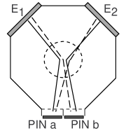
FIG. 12.: The data from two PINs at the same $z$-position in a proton segment can be used to cancel the effects due to the electron and neutrino asymmetries. The coincidences shown by solid lines (${\rm E}_{1}{\rm PIN}_{a}$ and ${\rm E}_{2}{\rm PIN}_{b}$) have approximately the same angle, a little less than 135^∘. These are referred to as “small-angle” coincidences. The “large-angle” coincidences for this pair of PINs (${\rm E}_{1}{\rm PIN}_{b}$ and ${\rm E}_{2}{\rm PIN}_{a}$) are the dashed lines.

We thus separate our data into a small-angle group and a large-angle group giving two statistically independent results for each PIN-diode–electron-detector pairing.

B Monte Carlo Methods

We use two Monte Carlo calculations to determine the values of ${K_{1}}$, ${K_{a}}$, ${{\mathbf{K}}_{A}}$, ${{\mathbf{K}}_{B}}$, and ${{\mathbf{K}}_{D}}$. The results from these two completely independent calculations are in excellent agreement. In both calculations neutron decay events are generated randomly within a trapezoid-cylindrical geometry (i.e. a tube with divergence) that can be offset with respect to the detector axis. A realistic beam profile, representative of Figure 4, can be modeled by combining results from several different trapezoids. In one of the Monte Carlo calculations the tracking of protons and electrons is done with the CERN Library GEANT3 Monte Carlo package [23], while in the other tracking is implemented within the code itself. In both, the emiT detector geometry is specified with uniform efficiency over the active area of each scintillator and over the square focusing region of each PIN diode.

The constants defined in Equation 9 are given by

$$K^{\alpha i}_{x}=\sum\delta^{\alpha i}X$$ (17)

where $X=1$, ${{\mathbf{p}}_{e}\cdot{\mathbf{p}}_{\nu}}/E_{e}E_{\nu}$, ${{\mathbf{p}}_{e}}/{E_{e}}$, ${{\mathbf{p}}_{\nu}}/{E_{\nu}}$, and ${{\mathbf{p}}_{e}\times{\mathbf{p}}_{\nu}}/{E_{e}E_{\nu}}$ for $x=1,~{}a,~{}A,~{}B,$ and $D$, respectively. We have studied systematic uncertainties associated with potential non-uniformities in the beta efficiencies and included them in the final uncertainty for the constants $K^{\alpha i}_{x}$. These constants (a total of 11, taking into account the three directions for each vector) are accumulated in a file that is read to calculate the factors $v$ (Equation 15) for different orientations of the polarization.

Values of $|{\tilde{\mathbf{K}}}^{\alpha i}_{D}\cdot{\hat{z}|}$ are used directly in the interpretation of the result for $D$. Variations among the PIN diode pairs of individual values of ${\tilde{\mathbf{K}}}^{\alpha i}_{D}$ within a given proton segment are negligible, and average values ($|\tilde{\mathbf{K}}_{D}\cdot\hat{z}|$) can be used. They are found to be $0.424\pm 0.010$ and $0.335\pm 0.020$, for the small- and large-angle coincidences, respectively. The uncertainties are primarily from uncertainties in the geometry of the beam. Values for the other $K^{\alpha i}_{x}$ are used in the estimation of systematic uncertainties described in the following section.

C Discussion of Systematic Uncertainties

The largest of the systematic effects can be shown to be the contributions to the $v$ (Equation 18) that arise due to the misalignment of the neutron polarization with respect to the detector axis. A transverse component of the polarization produces a significant contribution to $v^{b2:a1}$ because the vector differences ${{\tilde{\mathbf{K}}}^{b2}_{A}}-{\tilde{\mathbf{K}}}^{a1}_{A}$ and ${{\tilde{\mathbf{K}}}^{b2}_{B}}-{\tilde{\mathbf{K}}}^{a1}_{B}$ are predominantly perpendicular to the detector axis. (For example, ${{\tilde{\mathbf{K}}}^{b2}_{A}}-{\tilde{\mathbf{K}}}^{a1}_{A}$ is proportional to the integral of ${\mathbf{p}}_{e}(E_{1})-{\mathbf{p}}_{e}(E_{2})$ and is directed horizontally to the left in Figure 12. The difference ${{\tilde{\mathbf{K}}}^{b2}_{B}}-{\tilde{\mathbf{K}}}^{a1}_{B}$ is antiparallel to ${{\tilde{\mathbf{K}}}^{b2}_{A}}-{\tilde{\mathbf{K}}}^{a1}_{A}$.) For an azimuthally symmetric neutron beam, it can be shown that for each proton detector segment (labeled with subscripts $\eta$= I, II, III, IV) the weighted average of the $v^{\alpha i:\beta j}$ for all large or small detector pairs can be expressed as

$$v_{\eta}^{l/s}=PD(\tilde{\mathbf{K}}_{D}^{l/s}\cdot\hat{\sigma})+\alpha_{\eta}^{l/s}\sin\theta_{\sigma}\sin(\phi_{\eta}-\phi_{\sigma}),$$ (18)

where $\theta_{\sigma}$ and $\phi_{\sigma}$ are the polar and azimuthal angles of $\hat{\sigma}$, and $\phi_{\eta}$=0^∘, 90^∘, 180^∘, and 270^∘ respectively for detectors I, II, III, and IV. This dependence can be derived analytically for zero beam radius and is confirmed by Monte Carlo simulations for symmetric beams of finite radius. The coefficients $\alpha_{\eta}$ measure the combined effects of the $A$ and $B$ correlations for each proton detector segment.

If the symmetry of the four sets of proton detectors were perfect, i.e. $\alpha_{\rm I}=\alpha_{\rm II}=\alpha_{\rm III}=\alpha_{\rm IV}$, the contributions due to the $A$ and $B$ coefficients would average to zero, and Equation 16 would be valid, even with a polarization misalignment. In the absence of perfect symmetry, these contributions do not cancel when the four proton detectors are combined, and a false $D$ contribution would result from the application of Equation 16. This false $D$ is proportional to the product of two effects that are both small: the misalignment of the neutron polarization with respect to the detector axis ($\theta_{\sigma}$) and the departure from perfect symmetry of the proton detectors ($\Delta\alpha=1/2(\alpha_{\rm I}-\alpha_{\rm III})+1/2(\alpha_{\rm II}-\alpha_{\rm IV})$). Such an effect is called the “tilting asymmetric transverse polarization” effect, or “Tilt ATP”[9, 24].

The ATP effect was intentionally amplified for a systematic test, run with transverse polarization ($\theta_{\sigma}=90^{\circ}$ $\phi_{\sigma}=\phi_{\rm IV}=270^{\circ}$) and a distorted neutron beam. The neutron beam was distorted by blocking half of the beam with a neutron absorber placed upstream near the spin flipper. The results of this test are shown in Figure 13.

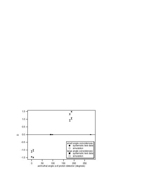
FIG. 13.: During the systematic test with a 90^∘ polarization tilt, the false $D$ in each proton segment is clearly visible. (The proton detector segment IV at $\phi_{\rm IV}$ = 270^∘ was not operational.) Also shown are the results of Monte Carlo simulations of the systematic test conditions. The error bars shown are purely statistical, and are not an accurate estimate of the total uncertainty in the calculation, of which the largest contribution is uncertainty about the shape of the beam.

This demonstration that the experiment can measure an asymmetry consistent with the Monte Carlo calculation serves as a strong check on both the operation of the detector and the validity of the analysis method.

A false $D$ also arises if the polarization has transverse components not described by a simple tilt. The form of Equation 18 shows that a net azimuthal component of $\hat{\sigma}$ also results in a contribution to $v_{\eta}$ that does not average to zero when data from proton segments I-IV are combined. This effect, referred to as a “twisting asymmetric transverse polarization” (“Twist ATP”) is shown by Monte Carlo simulations to be less than $10^{-4}$ for azimuthal polarizations of less than 1 mrad. For this reason, all sources of guide field distortion are kept to less than 1 mrad, and materials of low magnetic permeability (less than 0.005 $\mu_{0}$) were used in the detection region. There are exceptions to this requirement, however the net effect of all additional permeability was measured to produce less than 1 mrad of distortion of the guide field anywhere in the detector region.

Variations in the neutron flux ($\Phi$) and polarization ($P$) that depend on neutron helicity yield a false $D$. For this experiment the effects due to misalignment of the neutron spin are small[25], so that these systematic effects, to first order in $\Delta\Phi/\bar{\Phi}$ and $\Delta P$ are

$$D_{false}(\Delta\Phi)=\frac{\Delta\Phi}{\bar{\Phi}}PD{\hat{\sigma}}\cdot(A\langle{{\tilde{\mathbf{K}}}_{A}}\rangle+B\langle{{\tilde{\mathbf{K}}}_{B}}\rangle),$$ (19)

and

$$D_{false}(\Delta P)=\Delta PD{\hat{\sigma}}\cdot(A\langle{{\tilde{\mathbf{K}}}_{A}}\rangle+B\langle{{\tilde{\mathbf{K}}}_{B}}\rangle).$$ (20)

Here $\Delta\Phi=\Phi_{\uparrow}-\Phi_{\downarrow}$, and $\Delta P=P_{+}-P_{-}$. ($P$ in Equations 15 and 16 would be replaced by $\bar{P}=(1/2)[P_{+}+P_{-}]$.) The $\langle{{\tilde{\mathbf{K}}}_{A}}\rangle$ and $\langle{{\tilde{\mathbf{K}}}_{B}}\rangle$ are average values for all PIN-diode–electron-detector pairings.

Our data provide an upper limit of 0.002 for $P{\hat{\sigma}}\cdot(A\langle{{\tilde{\mathbf{K}}}_{A}}\rangle+B\langle{{\tilde{\mathbf{K}}}_{B}}\rangle)$. We combine this with neutron flux monitor data for $\Delta\Phi/\Phi<0.004$, concluding that $D_{false}(\Delta\Phi)<8\times 10^{-6}D$. The flipping ratio measurement has been used to derive a lower limit on the spin flipper efficiency of 82% so that $\Delta P<0.2$, and $D_{false}(\Delta P)<4\times 10^{-4}D$. We conclude that both effects are negligible in this measurement.

D Results

A final value of $D_{\eta}^{l/s}=v_{\eta}/(P\tilde{\mathbf{K}}_{D}^{l/s}\cdot\hat{z})$ is found separately for large angle and small angle pairings of each proton segment. The quantities $v_{\eta}$ are the weighted averages of all PIN-electron detector pairs, $v^{l/s}(\alpha i:\beta j)$, within each proton detector segment. Use of the weighted averages is justified because the systematic uncertainties described above have negligible variations among the PIN diode pairs in a given detector. The individual proton segment data ($v_{\eta}$) are then combined in an arithmetic average so that the sinusoidal variation given in Equation 16 cancels to first order in misalignments, i.e.

$$\sum_{\eta={\rm I}}^{\rm IV}v_{\eta}^{l/s}=4D^{l/s}(P{\tilde{\mathbf{K}}_{D}^{l/s}\cdot\hat{z}})+{\cal O}(\theta_{\sigma}\Delta\alpha).$$ (21)

The error for $D^{l/s}$ includes the uncertainty in the values of ${{\tilde{\mathbf{K}}}^{l/s}_{D}}\cdot\hat{z}$.

$$\sigma_{D^{l/s}}^{2}=\frac{1}{4P\tilde{\mathbf{K}}^{l/s}\cdot\hat{z}}\sum_{\eta={\rm I}}^{\rm IV}\sigma^{2}_{v^{l/s}}+D^{l/s}\bigg{(}\frac{\sigma_{|\tilde{\mathbf{K}}^{l/s}_{D}\cdot\hat{z}|}}{|\tilde{\mathbf{K}}^{l/s}_{D}\cdot\hat{z}|}\bigg{)}^{2}$$ (22)

Data for each proton segment are displayed in Figure 14, where we plot values for the eight individual $D_{\eta}^{l/s}$.

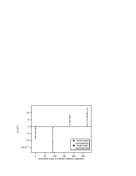
FIG. 14.: Results from each of the four proton segments for small-angle and large-angle PIN-electron detector pairs. $D_{\eta}^{l/s}=v_{\eta}/(P\tilde{\mathbf{K}}_{D}^{l/s}\cdot\hat{z})$. Error bars are statistical.

(The sinusoidal variation is predicted by Equation 18 and also seen in the test data of Figure 13, where the amplitude is 100 times larger.)

The two independent measurements for small angle and large angle PIN-electron detector pairs can be combined in a weighted average.

$$D=\frac{D^{s}/\sigma^{2}_{D^{s}}+D^{l}/\sigma^{2}_{D^{l}}}{1/\sigma^{2}_{D^{s}}+1/\sigma^{2}_{D^{l}}}$$ (23)

The full uncertainty includes the uncertainty from the average neutron beam polarization.

$$\sigma_{D}^{2}=\Big{(}\frac{1}{1/\sigma^{2}_{D_{(s)}}+1/\sigma^{2}_{D_{(l)}}}\Big{)}+\Big{(}D\frac{\sigma_{\bar{P}}}{\bar{P}}\Big{)}^{2}$$ (24)

The data are also analyzed by breaking each series up into individual runs and combining PIN-electron detector pairings in the same way. The results of these analyses are consistent. The final result is $(-0.6\pm 1.2)\times 10^{-3}$, where we have assumed the neutron polarization is $\bar{P}=(96\pm 2)$%. This is derived from our measurement of flipping ratio described in Section II A, with the assumption that the allowed range ($93\%\leq P\leq 100\%$) spans $2\sigma_{\bar{P}}$.

Finally, we use the scaled results from the systematic test data (Figure 13) combined with Monte Carlo simulation studies to estimate the uncertainty of the Tilt-ATP systematic effect. For the test data, proton detector IV ($\phi_{\rm IV}=270^{\circ}$) was not operational. In calculating $D$ for the test data, only values from detectors I and III can therefore be used in Equation 21 with a result of ${1\over 2}(D_{\rm I}+D_{\rm III})=(-6.5\pm 1.4)\times 10^{-2}$. Monte Carlo simulations show that for a beam of radius 3 cm, the $\sin(\phi_{\eta}-\phi_{\sigma})$ behavior of Equation 18 is modified so that $D_{test}={1\over 2}(D_{\rm I}+D_{\rm III})/1.6=(-4.1\pm 0.9)\times 10^{-2}$. This can be scaled by $\sin\theta_{\sigma}$, the ratio of polarization misalignments for the data and test runs. The individual values of $D_{\eta}^{l/s}$ shown in Figure 14 are used to determine $\theta_{\sigma}=(9\pm 3)\times 10^{-3}$ radians for the data run. This provides an upper limit for the uncertainty on the Tilt-ATP systematic effect of $D$(Tilt ATP)$<D_{test}\sin\theta_{\sigma}\leq 5.2\times 10^{-4}$. Though we use the test results to estimate this false $D$ effect, we expect the cancellation due to beam symmetry to be more complete for the data run because the test beam was intentionally distorted. We therefore consider this upper limit to be a conservative estimate of the largest possible false $D$ effect [26] The contributions to the statistical and systematic uncertainties are given in Table II.

Sources of uncertainty	Contribution ($\times 10^{-4}$)
Statistics	12
Tilt ATP	5
Twist ATP	$<$1
Flux variations	negligible
Polarization variations	negligible

TABLE II.: Contributions to the uncertainty.

V Summary and Conclusions

The apparatus used to perform a measurement of the $D$-coefficient in the beta-decay of polarized neutrons has been described. The data using the emiT detector have been analyzed using a technique that is insensitive to the nonuniform detection efficiency over the proton detectors. The initial run produced a statistically limited result of $D=[-0.6\pm 1.2({\rm stat})\pm 0.5({\rm syst})]\times 10^{-3}$. This result can be combined with earlier measurements to produce a new world average for the neutron $D$ coefficient of $-5.5\pm 9.5\times 10^{-4}$, which constrains the phase of $g_{A}/g_{V}$ to $180.073^{\circ}\pm 0.12^{\circ}$. This represents a 33% improvement (95% C.L.) over limits set by the current world average, and correspondingly further constrains standard model extensions with leptoquarks [18]. The result is also interesting in light of upper limits provided by the neutron and ¹⁹⁹Hg electric dipole moments on T-odd, P-even interactions such as left-right symmetric models and exotic fermion models.

A second run is being planned with strategies to improve the statistical limitations related to background experienced in the first run. Our study of systematic effects presented here shows that the largest is the tilt-ATP effect. The uncertainty on this effect can be reduced significantly with more data taken in the transverse polarization mode described in Section IV C. With the planned improvements in place, it will be feasible to improve the sensitivity to $D$ to $3\times 10^{-4}$ or less.

REFERENCES

- [1] J. H. Christenson, J. W. Cronin, V. L. Fitch, and R. Turlay, Phys. Rev. Lett. 13, 138 (1964); V. Fanti et al., Phys. Lett. B465, 335 (1999); A. Alavi-Harati et al., Phys. Rev. Lett. 84, 408 (2000).
- [2] A. Angelopoulos et al., Phys. Lett. B444 43 (1998); L. Alvarez-Gaume, C. Kounnas, S. Lola, P. Pavlopuolos, Phys. Lett. B458, 347 (1999).
- [3] M. Kobayashi and T. Maskawa, Prog. Theor. Phys. 49, 652 (1973).
- [4] A. Riotto and M. Trodden, Annu. Rev. Nucl. Part. Sci. 49, 35 (1999).
- [5] J. D. Jackson, S. B. Treiman, and H. W. Wyld, Jr, Nucl. Phys. 4, 206 (1957).
- [6] C. Caso et al., Eur. Phys. J. C 3 (1998) 1 and 1999 off-year partial update for the 2000 edition available on the PDG WWW pages (URL: http://pdg.lbl.gov/).
- [7] R. I. Steinberg, P. Liaud, B. Vignon, and V. W. Hughes, Phys. Rev. Lett. 33, 41 (1974).
- [8] B. G. Erozolimskii, Yu. A. Mostovoi, V. P. Fedunin, A. L. Frank, and O. V. Khakhan, Sov. J. Nucl. Phys. 28, 98 (1978).
- [9] B. G. Erozolimskii, Yu. A. Mostovoi, V. P. Fedunin, A. L. Frank, and O. V. Khakhan, JETP Lett. 20, 345 (1974).
- [10] H. Wenninger, J. Stiewe, and H. Luetz, Nucl. Phys. A109, 561 (1968).
- [11] A. S. Carnoy, J. Deutsch, and P. Quin, Nucl. Phys. A568, 265 (1994).
- [12] C. G. Callan and S. B. Treiman, Phys. Rev. 162, 1494 (1967).
- [13] A. L. Hallin, F. B. Calaprice, D. W. MacArthur, L. E. Piilonen, M. B. Schneider, and D. F. Schreiber, Phys. Rev. Lett. 52, 337 (1984).
- [14] J. Sromicki, M. Allet, K. Bodek, W. Hajdas, J. Lang, R. M ller, S. Navert, O. Naviliat-Cuncic, and J. Zejma, Phys. Rev. C 53, 932 (1996).
- [15] E. D. Commins, S. B. Ross, D. DeMille, B. C. Regan, Phys. Rev. A 50, 2960 (1994).
- [16] P. G. Harris et al., Phys. Rev. Lett. 82, 904 (1999).
- [17] J. P. Jacobs, W. M. Klipstein, S. K. Lamoreaux, B. R. Heckel, E. N. Fortson, Phys. Rev. A 52, 3521 (1995).
- [18] P. Herczeg, in Proc. of the 6th Int. PASCOS-98, ed. P. Nath, World. Sci., Singapore, (1998); For the limit in the Minimal Supersymmetric Standard Model see E. Christova and M. Fabbrichesi, Phys. Lett. B315, 113, (1993).
- [19] L. J. Lising, Ph.D. thesis, University of California at Berkeley (1999).
- [20] S. R. Hwang, Ph.D. thesis, University of Michigan (1998).
- [21] O. Schaerpf, Physica B 156-157, 631 (1989) and O. Schaerpf, Physica B 156-157 639 (1989).
- [22] Certain trade names and company products are mentioned in the text or identified in illustrations in order to adequately specify the experimental procedure and equipment used. In no case does such identification imply recommendation or endorsement by National Institute of Standards and Technology, nor does it imply that the products are necessarily the best available for the purpose.
- [23] Application Software Group, CERN Program Library Long Writeup W5013, CERN, Geneva (1993).
- [24] E. G. Wasserman, Ph.D. thesis, Harvard University (1994).
- [25] Exact expressions that do not require polarization misalignment effects to be small are and Here is given by equation 15, , and and would be measured with and .
- [26] The beam profiles were mapped at the entrance to the detector by measuring the flux through a pinhole as it was scanned in two dimensions across the beam. In both cases the beam profiles are highly symmetric. Even with half of the beam blocked, mixing in the downstream guide tubes gives a beam density with a center of mass displaced by only 2 mm from the beam axis. For the data run, the beam was centered to within 0.6 mm.