Measurements of Light Nuclei Production in 11.5 A GeV/c Au + Pb Heavy-Ion Collisions

Abstract

We report on measurements by the E864 experiment at the BNL-AGS of the yields of light nuclei in collisions of ${}^{197}Au$ with beam momentum of 11.5 A GeV/c on targets of ${}^{208}Pb$ and ${}^{197}Pt$. The yields are reported for nuclei with baryon number A=1 up to A=7, and typically cover a rapidity range from $y_{cm}$ to $y_{cm}+1$ and a transverse momentum range of approximately $0.1\leq p_{T}/A\leq 0.5$GeV/c. We calculate coalescence scale factors $B_{A}$ from which we extract model dependent source dimensions and collective flow velocities. We also examine the dependences of the yields on baryon number, spin, and isospin of the produced nuclei.

25.75.-q

I Introduction

Relativistic heavy ion collisions are believed to reach energy densities an order of magnitude greater than that of normal nuclear matter. These collisions allow the examination of the strong interaction in a novel environment as well as providing a possible doorway to new states of matter. In order to understand the dynamics of the collision system, one must use the only available tools-the species and momenta of the particles which exit the collision region. The use of emitted hadrons to probe the collision system is complicated because these hadrons rescatter many times as they traverse the collision region, and consequently lose some of their direct information about the earlier stages of the time evolution. However, the final space-time extent of the system at freeze-out (the time when strong interactions cease) and position-momentum correlations of the emitted particles contain much information about the entire time evolution. In principle, these carry information about the equation-of-state of the early collision region.

In order to extract information about both the momentum and position distributions of the source at freeze-out, it is necessary to measure multi-particle correlations. One widely used technique is Hanbury-Brown-Twiss interferometry [13] for which the correlations between particles are due to quantum statistics. Another method is through the measured yields of light nuclei, which are formed by the coalescence of individual nucleons.

Because of the violence of heavy ion collisions, it is highly improbable for a nuclear cluster near center-of-mass rapidity $y_{cm}$=1.6 in a collision at these energies to be a fragment of the beam or target nucleus [14] [15]. This would involve a cluster suffering a momentum loss of several GeV/c per nucleon that does not destroy the cluster, which is typically bound by only a few MeV per nucleon. These nuclei then are formed by coalescence and so represent correlations of several nucleons. As the mass of measured nuclei increases, of course, so does the number of particles involved in the correlation, and so does the sensitivity to features of the freeze-out distribution.

In part due to the fragility of these states, the observed light nuclei are believed to be formed only near freeze-out of the collision system, at which time the mean free path of a bound cluster is long enough for it to escape without further collision. It is this notion that gives rise to a class of models of light nuclei production, the coalescence models (for example, [16, 17, 18]). In general, these models assume a phase space distribution of nucleons at freeze-out and impose some coalescence conditions on the freeze-out positions and momenta of the nucleons in order to calculate the yields of nuclei. These models differ both in their assumptions about the phase space profiles and coalescence conditions. Their differences are often characterized by their predictions of the invariant coalescence, or $B_{A}$, parameters which are defined as

$$B_{A}\equiv\frac{(E\frac{d^{3}N_{A}}{dP^{3}})}{(E\frac{d^{3}N_{neutron}}{dp^{3}})^{N}(E\frac{d^{3}N_{proton}}{dp^{3}})^{Z}}$$ (1)

where a nucleus with baryon number $A$ and momentum $P=pA$ is formed out of $Z$ protons and $N$ neutrons.

In the simplest momentum space coalescence models, coalescence is assumed to take place between any nucleons with a small enough momentum difference. Early experimental results at the Bevalac with beam energies of $\approx 500A$MeV and high energy proton induced reactions revealed $B_{A}$ parameters which were approximately constant for these different collision systems ([19, 18] contain useful summaries). The assumption of such simple models is that if the collision spatial volume is similar to size of the cluster, all nucleons whose momentum difference is less than a fixed value will fuse to form a nuclear cluster. Thus the experimentally observed constant $B_{A}$ values may indicate collision volumes in these systems that are not substantially larger than the RMS size of a deuteron.

In more advanced models, assuming a quantum mechanical sudden approximation [17] and using a density matrix formalism, accounting for both the positions and momenta of the nucleons [16], the $B_{A}$ parameters take on a relationship with the source volume $V$ of $B_{A}\propto(1/V)^{(A-1)}$. Heavy-ion experimental results at higher energies at the AGS ($\approx 10AGeV$) and CERN ($\approx 160AGeV$) revealed $B_{A}$ values that decreased with beam energy. This observation was understood to be a sign of significant expansion in the collision volume before freeze-out. This larger source volume creates a situation where some nucleons with small relative momentum will have too large a spatial separation to coalesce, thus reducing $B_{A}$.

The density matrix formalism [16] assumes that although the collision volume can expand significantly, there is no correlation between the momentum and the position of a given particle. This assumption then leads to a prediction of no kinematic dependence of the $B_{A}$ parameter. However, there is a great deal of evidence that collective motion is present leading to expansion of the collision volume and significant position-momentum correlations [20] [21]. Although the overall expansion of the system tends to decrease $B_{A}$ values by spatially isolating nucleons from each other, collective motion makes it more likely that nucleons that are spatially close together also have similar momenta, which to some extent works in the opposite direction by increasing $B_{A}$. Other coalescence models have made an effort to include the effects of both larger source volumes and collective motion, by including coalescence as a ’afterburner’ in collision cascade models such as RQMD [22, 18] and by analytical calculations [23] [24].

Light nuclei production can also be calculated from thermal models [25] [26, 20] which assume at least local thermal equilibrium of the system and thus that particle production (including, in this case, composite particles) is governed by a single temperature and chemical potentials. This gives rise to expressions for the $B_{A}$ with the same $(1/V)^{(A-1)}$ dependence found in some coalescence models. Collective expansion can be included in these models ; it affects only the amount of energy available in local rest frames for particle production.

There has been much experimental effort in the measurement of light nuclei in heavy ion reactions. Previous measurements at AGS energies, including clusters of $A\leq 4$, show values for $B_{A}$ that are considerably lower than at Bevalac energies [27], indicating a much greater expansion of the system. This is also consistent with AGS results showing that the $B_{A}$ become smaller with more central collisions and larger target nuclei [28] [29]. At CERN-SPS energies, production of secondary particles (chiefly pions) is several times as large as at the AGS, leading to a larger expansion before hadronic freeze-out. Coalescence of high mass clusters is thus much less probable, as indicated by yet lower values for the $B_{A}$ as measured for example by experiment NA52 [19].

In this paper we describe and report the results of measurements by E864 of the yields of light nuclei in collisions of ${}^{197}Au$ with beam momentum of 11.5 A GeV/c on targets of ${}^{208}Pb$ and ${}^{197}Pt$. The yields are measured for nuclei from baryon number A=1-7. In Section II we briefly describe the experimental apparatus and the analyses used to produce our final invariant multiplicities. In Section III we report the results and compare them with measurements of other experiments where such measurements overlap. Finally in Section IV we examine trends in the data and discuss interpretations in the context of several different models of light nuclei production.

II Experiment 864

A Apparatus

Brookhaven AGS Experiment 864 is an open geometry, high data rate spectrometer which was chiefly designed to search for rarely produced objects in Au+Pb collisions. Figure 1 shows a schematic view of the experimental apparatus, a thorough description of which is given in [30]. Event centrality (impact parameter) is characterized by the charged particle multiplicity measured in an annular scintillator counter [31] located approximately 10 cm downstream of the target, which subtends an angular region from 16.6^o to 45^o in azimuth when viewed from the target. The products of an interaction travel downstream through two dipole spectrometer magnets, M1 and M2. Charged particle identification is performed using information from the scintillator hodoscope walls (H1, H2, and H3) and the straw tube stations (S2 and S3). The hodoscopes walls each consist of 206 1cm thick scintillator slats placed vertically. They provide information about the charge, time-of-flight, and position of each charged particle hit, and this information is used to identify candidate charged particle tracks. These tracks are then rejected or confirmed and further refined by spatial hit information provided by the straw tube stations. Under the assumption that the track originates in the target, a rigidity is assigned to the track by a look-up table generated from a GEANT simulation of the experimental apparatus (using a technique described in [32] as applied for the PHENIX experiment at RHIC). With information on rigidity, time-of-flight, and charge, a mass can then be assigned to the track, providing particle identification. A typical charge one mass distribution with a field of 0.45 Tesla in our spectrometer magnets is shown in Figure 2. Mass resolutions of 3 to 7% RMS are typical for particles with velocity $\beta\leq.985$.

At the downstream end of the apparatus is our hadronic calorimeter [33]; an array of 754 towers, each measuring 10cm x 10cm on the front face, each of which provides energy and time information. This is the essential piece of the apparatus in our analyses of yields of neutral particles, for which the tracking detectors serve only to provide a veto. In addition, the energy and timing information from each tower is used to provide the input for a level II high mass trigger (the Late-Energy Trigger or LET [34]), which provides an enhancement of approximately a factor of 50 in our searches for rare high mass states.

Measurements reported in this paper are from a variety of experimental conditions, including different trigger conditions and different magnetic field settings in M1 and M2. The different data sets and their experimental conditions are listed in Table I. Because of the large acceptance open geometry design of the experiment, the different data sets often have significant regions of overlap with one another, allowing a consistency check on the measurements-see for example the measurements of alpha particles introduced in Section III.

B Data Analysis

In order to measure the yield of a given species, a mass plot analogous to Figure 2 is made for each kinematic bin. The number of tracks which lie within its mass peak are determined. Background under each peak is then estimated, generally with fits to signal plus background, and subtracted away from this count. The invariant multiplicity in a given kinematic bin is then determined by correcting this number of raw counts for the geometric acceptance, trigger efficiency, charge cut efficiency, track quality cut efficiency, and detector efficiency.

Geometric acceptances are generally 25% or lower as shown in Figure 3 for protons. Charge cut and track quality cut efficiencies are typically 90 to 95%. The three redundant charge measurements for each track allow easy calculation of the charge cut efficiency in each hodoscope simply by examining charge measurements made in each hodoscope against results from the other two; charge misidentification in each of the three hodoscopes is less than one percent, so fewer than one track in a million is assigned an incorrect charge. In general, the track quality cuts are determined by comparison with monte-carlo simulations. In cases where the efficiencies are particularly high, they are determined directly from the data. The total track detector efficiency is 85 to 90%; this is determined by excluding each detector in turn from the track-finding process.

The trigger efficiency is significant only for those measurements which were made using the LET. This mass and momentum dependent efficiency ranges from approximately 40% to 90% for the measurements reported here. The LET efficiency is determined by two methods. The first, used mainly for slow, high mass states for which the efficiency is very high, is done simply using a monte-carlo simulation of the shower generated by the object and knowledge of the LET look-up table in each tower. The second method is from the equation $\epsilon_{LET}=N_{LET}/(N_{LET}+R\times N_{nonLET})$ where R is the rejection factor provided by the LET (i.e. number of events which fire the LET divided by the total number of events). $N_{LET}$ and $N_{nonLET}$ are the numbers of particles of interest which do and do not produce LET triggers in LET triggered events, respectively.

Sources of systematic error that we have quantified include possible error in the determination of the efficiencies listed above as well as error in background subtraction (particularly relevant for the deuterons and alpha particles at their highest rapidities). Also examined were the effects of changing the assumed input distribution for each particle species in the determination of geometrical acceptances and efficiencies and effects of possible differences in the magnetic field with the field maps that were used in reconstruction of tracks.

Overall errors are generally dominated by systematics, particularly for the lighter states. Statistical errors can be significant for the heavier states, particularly in the determination of LET efficiencies in which the number of particles of interest which do not fire the LET generally has the largest statistical error.

III results

Measurements of invariant multiplicities for protons, neutrons, deuterons, ${}^{3}He$, and ${}^{4}He$ are shown in Figures 4 through  9, and the values of the data shown in these figures are listed in tables in the Appendix. Figure 4 displays proton invariant multiplicities for three different bins of collision centrality. Figure 5 shows only proton yields from 10% most central Au+Pb collisions along with neutron multiplicities measured by E864 (see Reference [35]) for comparison. Figures 6 and 7 display deuteron and ${}^{3}He$ invariant multiplicities for the same centrality bins used for the proton measurements. Tritons, ${}^{4}He$, ${}^{6}He$, ${}^{6}Li$, ${}^{7}Li$, and ${}^{7}Be$ are measured by E864 only in 10% most central collisions; yields for tritons and alpha particles are shown in Figure 8 and Figure 9, respectively, while yields for the heavier nuclei are listed in tables in the Appendix. Added detail concerning most of these measurements may be found in the Ph.D. theses listed in Reference [36].

A Contributions from Hyperon Decays

For comparison to other experimental results and calculations of coalescence parameters, it is important to quantify the contribution to proton yields that is made by protons which come from decays of hyperon states, which to E864 are indistinguishable from primordial protons. There are three dominant hyperon decays which produce protons: $\Lambda\rightarrow p+\pi^{-}$, $\Sigma^{0}\rightarrow\Lambda+\gamma\rightarrow p+\pi^{-}+\gamma$, and $\Sigma^{+}\rightarrow p+\pi^{0}$. The contributions from these decays were evaluated using a GEANT simulation of the experiment with an input distribution taken from measurements of E891 for the Lambda [37] and an input distribution from RQMDv2.3 [22] for the Sigma. From this simulation it was determined that protons from hyperon decays account for approximately 12% of the measured yields of protons with only a slight kinematic dependence. The proton and neutron yields from E864 shown in Figures 4 and 5 have not been corrected for hyperon feed-down (nor have the values listed in the appendix tables).

B Comparisons with Other Experimental Results

Figure 10 shows a comparison of the light nuclei measurements from AGS experiments E864, E877 [38], and E878 [28]. Because of the different beam momenta of the experiments (10.8 A GeV/c in E878), the yields are plotted versus beam normalized rapidity. The yields shown for E864 and E877 are average yields at approximately $p_{T}/A$ = 150 MeV/c, while the E878 yields are measurements at $p_{T}\simeq 0$. Other caveats to the comparisons of the yields shown in Figure 10 are noted in the figure caption.

Proton yields measured by E864 are clearly higher than measurements by E878. Some of this difference can be attributed to protons which are feed-down from hyperon decay. The acceptance of E878 for these feed-down protons is only about 10% of what it is for primordial protons, while in E864 the two acceptances are nearly the same. When this difference is taken into account (see Section III A) and the E864 yields of primordial protons are lowered by approximately 12%, the results of the two experiments are different by approximately 25% at midrapidity; this lies within the range of systematic errors for the two experiments. At higher rapidities, the agreement is better.

Comparison of the three experiments’ measurements of deuterons and tritons shows close agreement and the measurements of E864 and E878 of alpha particle yields also agree within errors.

IV Discussion

A General Trends of the Spectra

1 Transverse Dependence of Yields

E864 has sufficient coverage in transverse momentum for us to extract measurements of inverse slope parameters of the different light nuclei yields in the rapidity range $2.2\leq y\leq 2.4$. Shown in Figure 11 are yields of protons, deuterons, ${}^{3}He$, and ${}^{4}He$ as a function of transverse mass $m_{T}-m_{0}=\sqrt{p_{T}^{2}+m_{0}^{2}}-m_{0}$ in this rapidity slice. Overlayed on the measurements are fits of each species to a Boltzmann distribution in transverse mass, from each of which we extract an inverse slope parameter, $T$, as noted in Figure 11. The fits from which we extract $T$ are linear fits to the log of the invariant multiplicities divided by $m_{T}$; this is the same fitting method used for determining the slope parameters for neutrons in [35]. The $\chi^{2}$ values are less than one per degree of freedom for all these fits.

These slope parameters, as well as those for neutrons in this same rapidity range, are displayed in Figure 12 as a function of mass number. Polleri et. al. [24] have demonstrated the sensitivity of these trends in the inverse slopes to the density and velocity profiles of the nucleons at the time when coalescence occurs. To make this point, they have performed calculations of the behaviour of these trends for different assumptions about the source distributions. Two of these assumptions give rise to the two curves shown overlayed on the data in Figure 12. The first has a ’box’ spatial profile and a linear velocity profile, and the second has a Gaussian spatial distribution and a velocity profile $v(r_{T})\propto r_{T}^{(1/2)}$. In determining the curves shown in Figure 12 we have fit the data to these two different functional forms with the numerical constraint of T=100 MeV for zero mass. Neither of these sets of model parameters provides an adequate description of the data. These curves are meant only to illustrate the sensitivity of these measurements: clearly, the sensitivity to the differences in these assumptions increases with increasing mass of the measured nuclei.

Shown in Figure 13 are these same trends in light nuclei slope parameters including centralities other than the 10% most central collisions. For the more peripheral events, the trends are consistent with a linear dependence of slope parameter on mass (matching the calculation in Reference [24] including box density profiles). Only for the most central events is there a clear rollover in the slope as a function of mass.

2 Longitudinal Dependence of Yields

In order to examine the rapidity dependence of the yields of light nuclei, we observe the trends in multiplicities in the $p_{T}/A$ range from 100 to 200 MeV/c. (Our transverse coverage is not sufficient to integrate in transverse momentum for a full measurement of dN/dy over this entire rapidity range.) In Figure 14 we show the invariant multiplicities of deuterons for this low $p_{T}$ range for three different centralities as a function of rapidity. The yields are concave as a function of rapidity (i.e. they are lowest at center-of-mass and increase toward beam or target rapidity) and become more concave for the more peripheral events. We can parameterize this concavity by fitting each set of yields to a quadratic $a+b(y-y_{cm})^{2}$. These fits are shown overlayed on the data in Figure 14. The ratio of coefficients, $b/a$, from this parameterization serves as a measure of the relative concavity of a species’ spectrum as a function of rapidity at low $p_{T}$ [39].

Values of this ratio $b/a$ are plotted in Figure 15 as a function of mass number $A$ for protons, deuterons and ${}^{3}He$ in three different collision centralities. We observe that the concavity of a spectrum increases with the mass of a species and with collision centrality. This can be understood as some form of collective motion in the longitudinal direction, either expansion or incomplete stopping, which increases in peripheral events. It also is consistent with a rapidity dependent transverse expansion which pushes the nuclei out of the transverse momentum range measured here.

B $B_{A}$ parameters

The trends noted in Section  IV A will also be observable in a study of the behaviour of the $B_{A}$ parameters. For simplicity, we can from our neutron measurements [35] characterize the neutron spectrum as a factor of 1.19$\pm$.08 greater than the proton spectrum (feed-down from hyperons is taken into account in determining this ratio), and so we evaluate $B_{A}$ as

$$B_{A}\equiv\frac{(E\frac{d^{3}N_{A}}{dP^{3}})}{(1.19)^{N}(E\frac{d^{3}N_{proton}}{dp^{3}})^{A}}.$$ (2)

for a nucleus of baryon number $A$ with $N$ neutrons and $Z$ protons. Again, all invariant yields are evaluated at a common velocity.

In Figures 16 and 17 we show measurements of $B_{2}$ and $B_{3}$ as a function of rapidity and transverse momentum. Because nucleons which are feed-down from weak decays are not available as nucleons for coalescence, we have subtracted the contribution to proton and neutron invariant yields from hyperon feed down for the calculation of $B_{A}$.

The values of the $B_{A}$ in Figures 16 and 17 are clearly not momentum independent as is assumed in many early coalescence models ([16] and [17], for example). This is expected given the large amount of evidence for collective flow in heavy-ion collisions [20]. The values of the $B_{A}$ parameters seem to increase slightly with increasing transverse momentum and there is a clear increase away from center-of-mass rapidity. Both of these increases in $B_{A}$ away from center-of-mass momentum are consistent with expectations from an expanding source, although the longitudinal dependence can also be interpreted as a sign of incomplete stopping. Indeed the fact that the invariant yields of antiprotons near $p_{T}$=0 are strongly peaked near center-of-mass rapidity as measured by E864 [40] while the proton yields are essentially flat may be taken as further evidence of incomplete stopping.

C Source Size Calculations

The $B_{A}$ parameters can be related through coalescence models to source sizes. Following the model of Sato and Yazaki [16] which uses a density matrix representation of the source distribution and projects it onto a representation of the deuteron wave function, we can relate the $B_{A}$ parameters to the RMS source radius through

$$B_{A}=(\frac{2J_{A}+1}{2^{A}})\frac{A^{5/2}}{m^{(A-1)}}(4\pi\frac{\nu_{A}\nu}{\nu_{A}+\nu})^{(3/2)(A-1)}$$ (3)

with $\nu_{A}$ the size parameter for a cluster with baryon number $A$ and spin $J_{A}$ ($m$ represents the nucleon mass). This model assumes the absence of collective motion of the nucleons, and therefore a radius (given by $R_{RMS}=\sqrt{3/2\nu}$) which is independent of momentum. We evaluate the source size using $B_{2}$, $B_{3}$, $B_{4}$, $B_{6}$, and $B_{7}$ values from our measurements nearest the collision center-of-mass (again assuming a neutron to proton ratio of 1.19) and list the results in Table II. We have used values for the $\nu_{A}$ from [16] for $A$ = 2,3 and 4 and following [41] have done a polynomial extrapolation to determine $\nu_{6}$ and $\nu_{7}$. This extrapolation for $\nu_{A}$ may be suspect particularly for the halo nucleus ${}^{6}He$, but the final value for $R_{RMS}$ is quite insensitive to the value for $\nu_{6}$. The extracted radius for deuterons $A$=2 is considerably larger than the initial size of the colliding nuclei, and the radius parameters decrease for clusters of increasing mass.

A model by Scheibl and Heinz [23] which includes the effect of collective flow in a density matrix prescription for coalescence leads to an expression for source dimensions:

$$B_{2}=\frac{3\pi^{3/2}<C_{d}>}{2m_{T}R_{\perp}^{2}(m_{T})R_{\parallel}(m_{T})}e^{2(m_{T}-m)(\frac{1}{T_{p}^{*}}-\frac{1}{T_{d}^{*}})}$$ (4)

where $R_{\perp}$ and $R_{\parallel}$ are the transverse and longitudinal dimensions of the fraction of the source which contributes to deuteron emission (comparable to the radius parameters extracted in the YKP parameterization of HBT interferometry), $<C_{d}>$ is a quantum mechanical correction factor for the finite size of the deuteron which is evaluated by the authors under various assumptions about the source, and $T_{p}^{*}$ and $T_{d}^{*}$ are the inverse slope parameters for protons and deuterons. Equation 4 as written assumes a box density profile for the source; a Gaussian profile would result in the absence of the final exponential factor. Plugging in our results for $B_{2}$, we can extract values for $(R_{\perp}^{2}(m_{T})R_{\parallel}(m_{T}))^{1/3}$ which are shown in Figure 18 as the solid circles. For the calculations shown here we have used 0.75 for $<C_{d}>$ and the values for $T_{d}^{*}$ and $T_{p}^{*}$ as measured at rapidity 2.3.

Shown also in Figure 18 as hollow circles are the results of source size calculations with the similar fragment coalescence model of Llope et. al. [41] via the equation

$$R_{c}^{3}=\pi^{3/2}\frac{(2J_{c}+1)}{(2J_{a}+1)(2J_{b}+1)}\frac{m_{c}}{m_{a}m_{b}}\frac{E_{a}\frac{d^{3}N_{a}}{dp_{a}^{3}}E_{b}\frac{d^{3}N_{b}}{dp_{b}^{3}}}{E_{c}\frac{d^{3}N_{c}}{dp_{c}^{3}}}$$ (5)

which relates the effective source radius $R$ in the frame of a cluster $c$ which may be formed through the coalescence of smaller clusters $a$ and $b$. (Note that the radius parameters $R$ shown in Figure 18 are meant to describe sources of the form $\rho(r)\propto exp(-r^{2}/2R^{2})$ and so correspond to RMS radii of $R_{RMS}=\sqrt{3}R$.)

We observe in Figure 18 that there is a decrease in source size with increasing distance away from the center-of-mass (again, as expected for a source with radial expansion), but our measurements do not give a clear picture concerning scaling of the source size with transverse mass [39] such as has been noted in results for sizes from HBT two-particle correlations and in measurements of $B_{2}$ at the CERN SPS [42].

D Comparison with RQMD

We can also compare our results with predictions from the cascade model RQMD [22] version 2.3. The complex many-body processes by which light nuclei are formed are not included in RQMD, rather an afterburner [43] is used to calculate the coalescence of these states based upon an input of the positions and momenta of the nucleons at freeze-out. This model then explicitly includes the position-momentum correlations due to expansion, etc. that are present in RQMD.

Figure 19 displays the E864 measurements along with predictions from RQMD with the coalescence afterburner for comparison over the transverse momentum range $0.1\leq\ p_{T}/A\leq 0.2$ GeV/c as a function of rapidity. For comparison, RQMDv2.3 was run under two different conditions, one including the effect of repulsive mean-field potentials (potentials mode) and one not (cascade mode). We note that there is an increasing disagreement with increasing mass as noted previously in Reference [28]. Calculations of ${}^{4}He$ production in cascade mode are at a level of approximately 100 lower than our measurements; with potentials on, the discrepancy is still larger by about a factor of two. The level of disagreement varies somewhat in with transverse momentum (the slopes are in fact generally better predicted with potentials on than off) but particularly for the heavier states the change is slight compared to the overall level of disagreement.

E Scaling of Yields Versus Mass

Shown in Figure 20 are the invariant yields in a small kinematic region at or near $y=1.9,p_{T}\leq 300MeV$. Over ten orders of magnitude, the yields in this kinematic bin fit very closely to an exponential dependence with a penalty factor of approximately 48 for each nucleon added (see [44] and references therein for a discussion of such exponential behavior of cluster yields at lower collision energies). Of course, as we have seen above, the yields for different species have different kinematic dependences due to collective motion, and so this should not be taken as a penalty factor which governs the integrated yields of the various species, which from the kinematic dependences of the $B_{A}$ parameters discussed in Section IV B can clearly be different.

We can make a crude estimate of the difference in these two penalty factors by parameterizing the rapidity and mass dependences of the inverse slope parameters as follows: from our neutron measurements [35] which extend up to beam rapidity, we can roughly parameterize the distribution of T in rapidity as a Gaussian with a width of 1.1 units. From Figure 13, we also can make a rough parameterization of the mass dependence of the inverse slope as $T\propto(A+1.0)$ With these two parameterizations and our penalty factor of 48 at $y=1.9,p_{T}\leq 300MeV$, we calculate a penalty factor of 25 in the integrated yields for the addition of an extra baryon to a coalesced state. This should be considered as a lower limit on such a penalty factor since as previously noted the inverse slope parameter rolls over as a function of mass rather than following the linear dependence we have used in this estimate [45].

We can also estimate this penalty factor in overall yields by following section VI of Reference [23]. Equation 6.10 in this reference allows us effectively to make an estimate of the difference between the penalty factor near $p_{T}$ = 0 and the overall penalty factor in two limiting cases: a static, homogeneous fireball (which would translate our penalty factor of 48 at $p_{T}$ =0 to an overall penalty factor of 72) and a rapidly expanding system (which would result in an overall penalty factor of 39).

F Spin and Isospin Dependences of Yields

In Figure  21, we display three ratios as a function of transverse momentum in the rapidity ranges y=1.8-2.0 and y=2.0-2.2. The three ratios are the ratios of invariant yield of neutrons over invariant yield of protons, the ratio of yield of tritons over yield of ${}^{3}He$ and the ratio of ${}^{6}He$ to ${}^{6}Li$. The $n/p$ and $t/^{3}He$ ratios are consistent with a value of approximately 1.2 (in Reference [35], we extract values of $1.19\pm.08$ and $1.23\pm.04$, respectively, for the two ratios in the range $1.6\leq y\leq 2.4$.). In contrast, the ${}^{6}He/^{6}Li$ is much nearer to a value of 0.3. $p$, $n$, ${}^{3}He$ and $t$ are all spin J=1/2 states while ${}^{6}He$ is spin 0 and ${}^{6}Li$ is spin 1. We take this as evidence that the yields scale as the degeneracy factor 2J+1 which is commonly predicted in thermal and coalescence models.

With the dependences upon mass number, isospin and spin divided away one can examine the yields for other dependences. This topic, including a possible dependence on binding energy per nucleon with an inverse slope parameter dependence of a few MeV, is discussed in Reference [46].

V Summary

We have shown results of measurements of light nuclei from $A$=1 to $A$=7. The increase with mass of light nuclei inverse slope parameters appears to roll over at approximately $A$=3 in central events but not necessarily in more peripheral events. Also we have shown that the yields near $p_{T}$=0 are concave as a function of rapidity and that this relative concavity increases in more peripheral events and in higher mass nuclei, consistent with both radial expansion and incomplete stopping. These trends are also evident from our observations of the kinematic dependences of the $B_{A}$ parameters. From these parameters we have extracted source dimensions from various models. Efforts to extract more quantitative information about the source from these measurements using the cascade model RQMD with a coalescence afterburner were unsuccessful as predictions of the model differ from our results by an amount that increases with mass and reaches a level of 100 or more by $A$=4.

We have also examined the overall scaling of the yields up to $A$=7, extracting a penalty factor of about 48 to add a nucleon to a coalesced state near midrapidity at low transverse momentum. This likely translates into a somewhat smaller penalty factor in overall yields for the addition of a nucleon, but we have argued that this is unlikely to differ by as much as a factor of two from our measured penalty of 48.

VI Acknowledgements

We gratefully acknowledge the efforts of the AGS staff in providing the beam. This work was supported in part by grants from the Department of Energy (DOE) High Energy Physics Division, the DOE Nuclear Physics Division, and the National Science Foundation.

VII APPENDIX

Shown in Table III through Table XVI are results of measurements by E864 of invariant multiplicities of light nuclei from $A$=1 through $A$=7 in 10% most central Au+Pb collisions. Results for less central data are also listed for protons, deuterons and ${}^{3}He$.

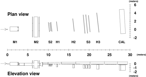
FIG. 1.: The E864 spectrometer in plan and elevation views, showing the dipole magnets (M1 and M2), hodoscopes (H1, H2, and H3), straw tube arrays (S2 and S3) and hadronic calorimeter (CAL). The vacuum chamber is not shown in the plan view.

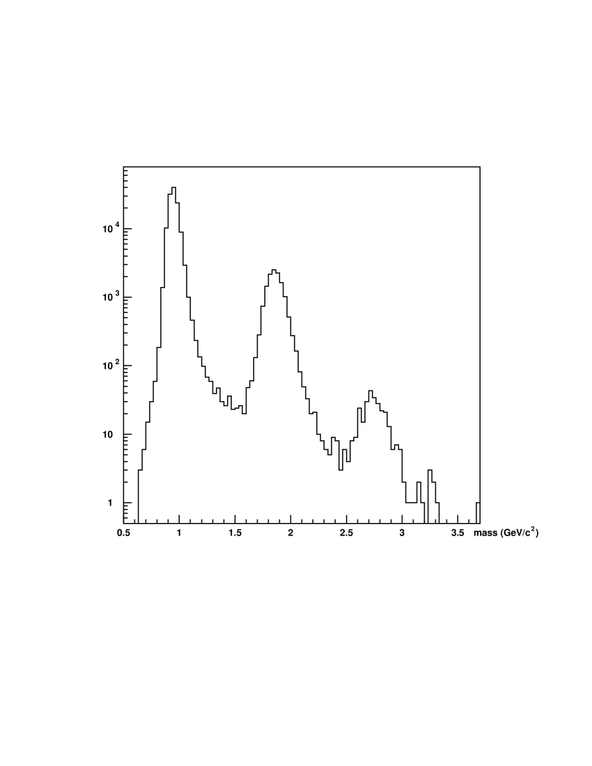
FIG. 2.: Typical reconstructed mass spectrum for charge one species in the rapidity slice $2.0\leq y\leq 2.2$ with a magnetic field of .45 T.

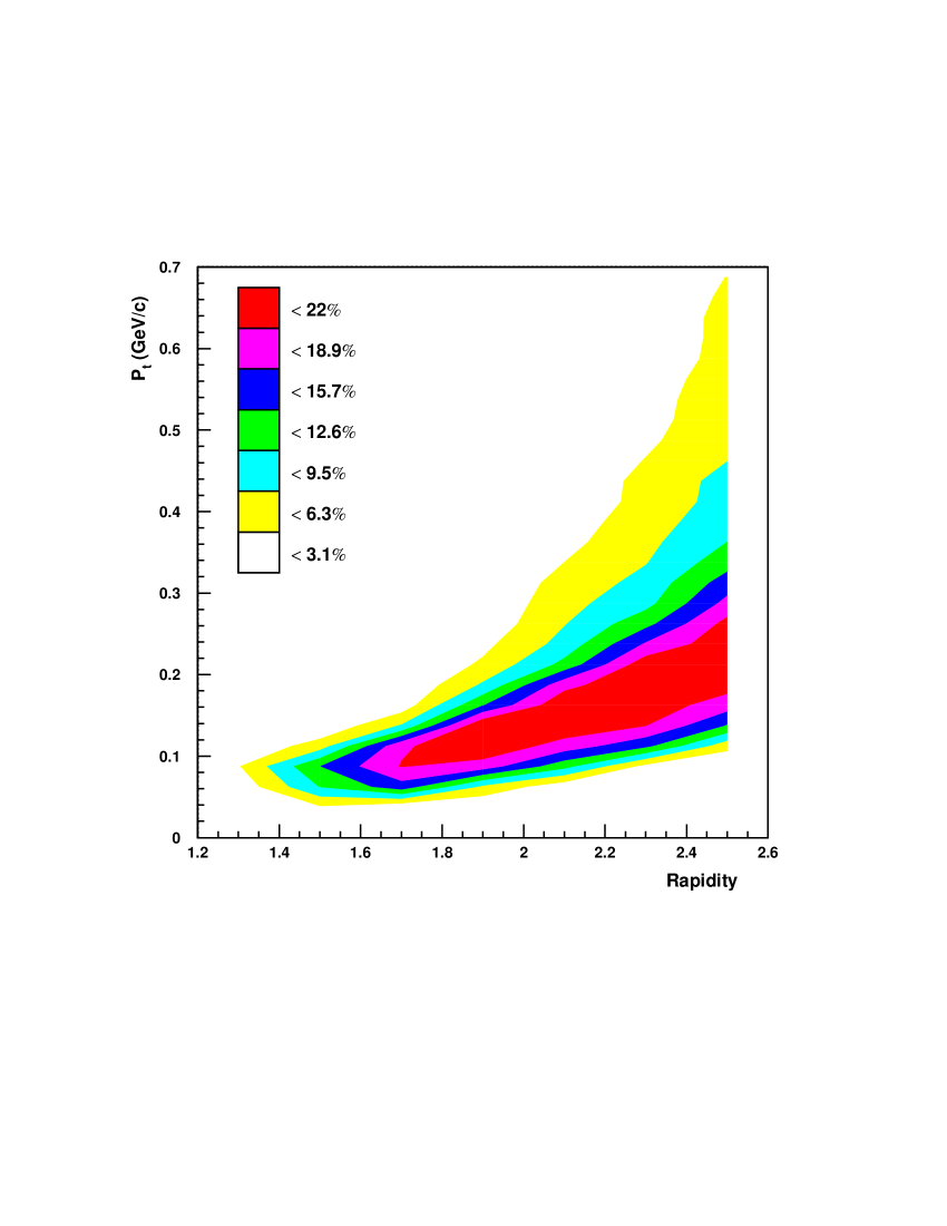
FIG. 3.: Geometric acceptance efficiency for protons in the B=.45 T field setting.

FIG. 4.: Panel (a) displays invariant yields for protons in 10% most central Au+Pb collisions. Panels (b) and (c) display the same for 10-38% and 38-66% central collisions, respectively.

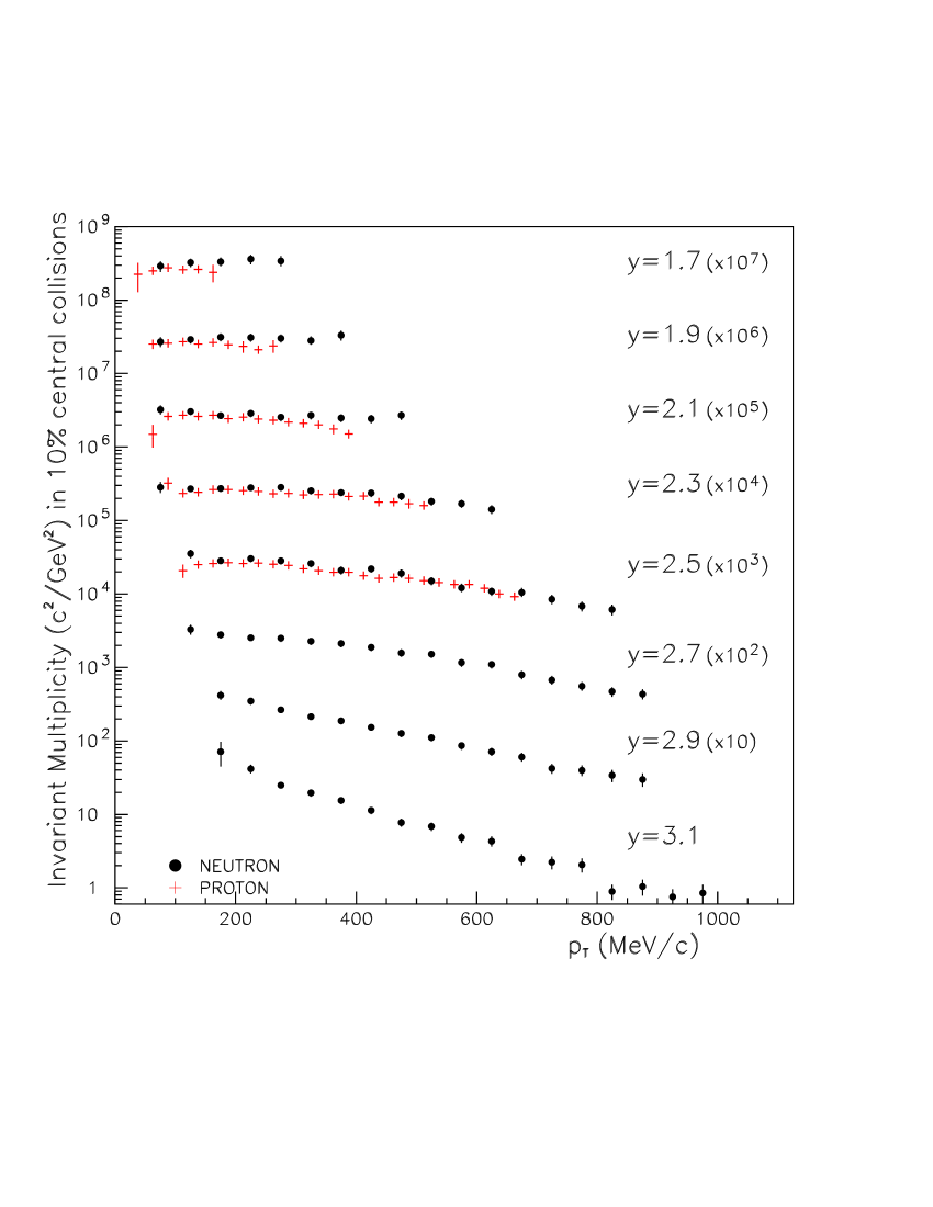
FIG. 5.: Invariant yields of protons and neutrons in 10% most central Au+Pb collisions.

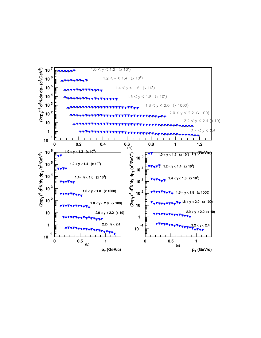
FIG. 6.: Panel (a) displays invariant yields for deuterons in 10% most central Au+Pb collisions measured by E864. Panels (b) and (c) display E864 measurements of deuteron invariant yields for 10-38% and 38-66% central collisions, respectively.

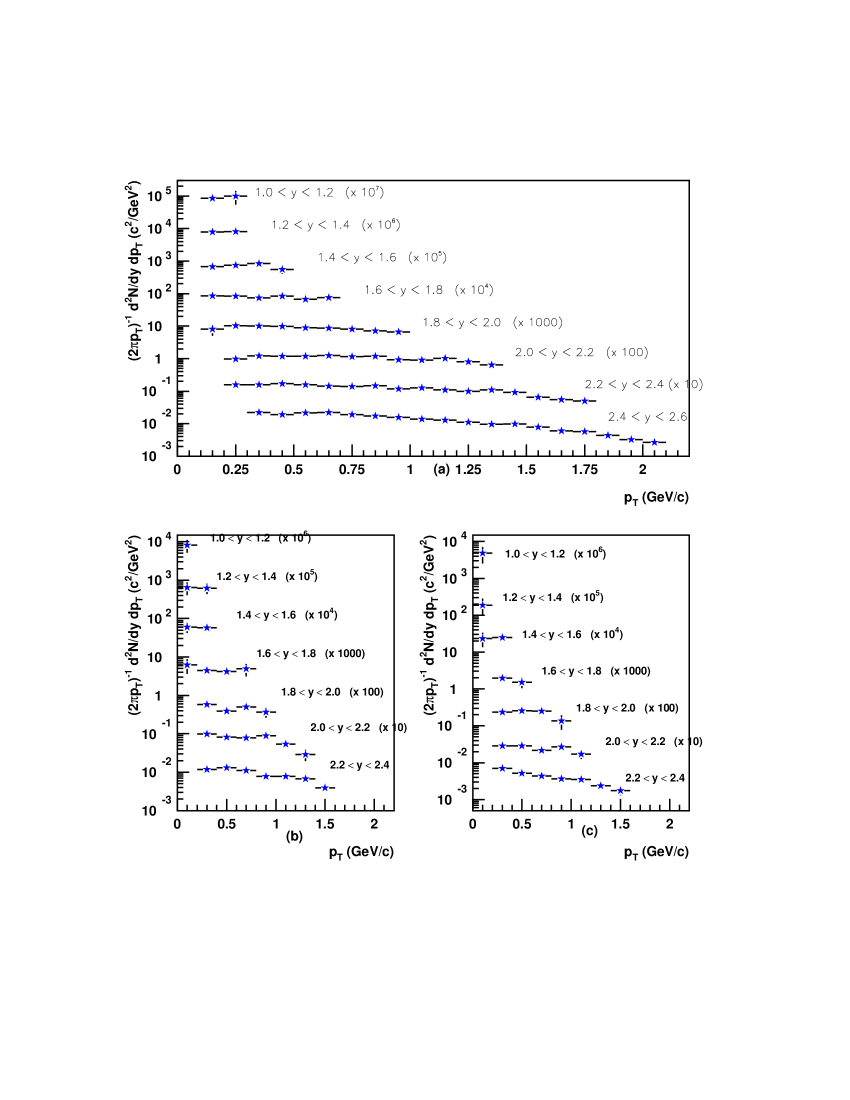
FIG. 7.: Panel (a) displays invariant yields for ${}^{3}He$ nuclei in 10% most central Au+Pb collisions. Panels (b) and (c) display the same for 10-38% and 38-66% central collisions, respectively.

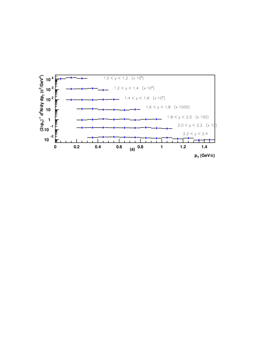
FIG. 8.: Invariant yields for tritons in 10% most central Au+Pb collisions.

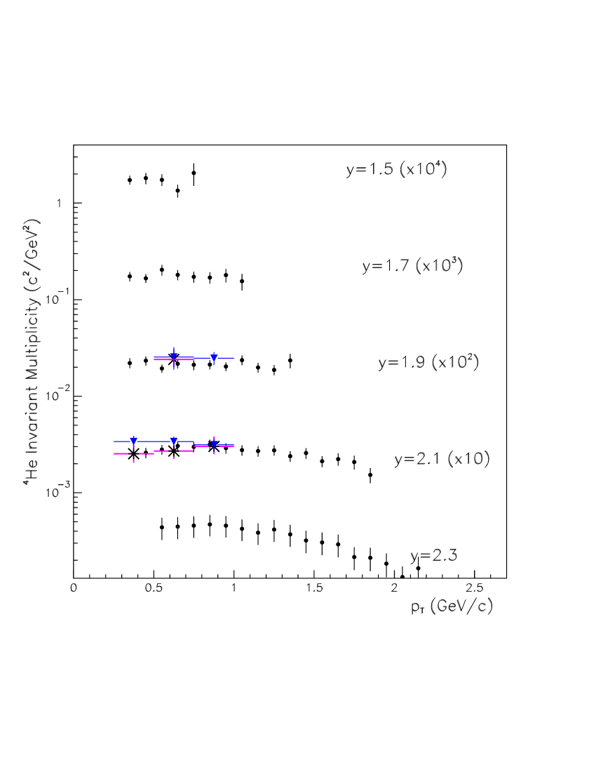
FIG. 9.: Invariant yields for alpha particles in 10% most central collisions. Solid circles represent measurements from data taken in the 1998 run (with a +.45 T field in M1 and M2) , triangles are measurements from the 1996 run (+1.5T field) and stars are measurements from the 1995 run (+1.5 T field). The larger uncertainties in the data points at rapidity 2.3 are due to increased contamination from ${}^{3}He$ at this rapidity. 1995 data is from Au+Pb while 1996 and 1998 data are from Au+Pt.

FIG. 10.: Comparison of light nuclei yields measured by E864, E877 and E878. The E864 results (solid circles) are the average of the yields over the transverse momentum range $.1\leq\frac{p_{T}}{A}\leq.2$ GeV/c. The E878 results (hollow squares) are the yields measured at $p_{T}\simeq 0$. The E877 points (hollow triangles) are measurements at $.15\leq\frac{p_{T}}{A}\leq.16$ GeV/c for deuterons and $.11\leq\frac{p_{T}}{A}\leq.22$ for tritons. E864 and E878 points represent yields in 10% most central collisions while E877 points are from 4% most central collisions. The E878 error bars are total errors including systematic errors except for the alpha particle yields which contain an additional 25% systematic error which is not shown. E864 error bars include both statistical and systematic errors.

FIG. 11.: Invariant yields of protons, deuterons, tritons, ${}^{3}He$ and ${}^{4}He$ in the rapidity range $2.2\leq y\leq 2.4$. Shown overlayed on each species is a fit to the spectrum assuming a Boltzmann distribution in transverse mass, with the extracted effective temperatures as noted.

FIG. 12.: Inverse slope parameters in the rapidity bin $2.2\leq y\leq 2.4$ shown as a function of mass number for protons, neutrons, deuterons, tritons, ${}^{3}He$, and ${}^{4}He$. Overlayed on the points are curves generated by assuming (i) a box density profile which gives rise to the straight line and (ii) a Gaussian profile with velocity profile $v_{\perp}\propto(r/R)^{(1/2)}$.

FIG. 13.: Inverse slope parameters for protons, deuterons, and ${}^{3}He$ in the rapidity bin $2.2\leq y\leq 2.4$ for three different collisions centralities.

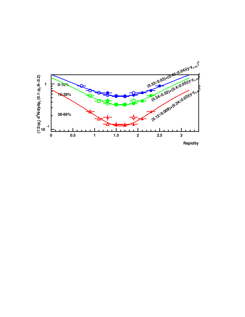
FIG. 14.: Invariant yields of deuterons in the range of transverse momentum $100\leq\frac{p_{T}}{A}\leq 200$ MeV/c as a function of rapidity for three different event centralities.

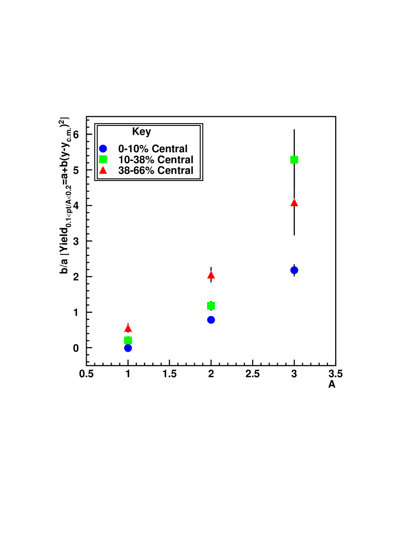
FIG. 15.: Relative concavity of light nuclei spectra as a function of rapidity plotted versus mass number $A$ for three different collision centralities.

FIG. 16.: Coalescence $B_{2}$ parameters, with an assumed neutron to proton ratio of 1.19, shown (a) as a function of transverse momentum in several rapidity slices and (b) as a function of rapidity near $p_{T}=0$. In panel (a), error bars include only point-to-point errors (a rapidity dependent error of 5% and a global 6% error are not included). In panel (b), hollow points represent reflections about center-of-mass rapidity. Here, the rapidity-dependent errors are included but the 6% global systematic error is not.

FIG. 17.: Coalescence $B_{3}$ parameters, with an assumed neutron to proton ratio of 1.19, shown (a) as a function of transverse momentum in several rapidity slices and (b) as a function of rapidity near $p_{T}=0$. In panel (a), error bars include only point-to-point errors (a rapidity dependent error of 8% and a global 11% error are not included). In panel (b), hollow points represent reflections about center-of-mass rapidity. Here, the rapidity-dependent errors are included but the 11% global systematic error is not.

FIG. 18.: Radius parameters extracted from measurements of $B_{2}$ within the context of two different models. The solid circles are to be understood as $(R_{\perp}^{2}(m_{T})R_{\parallel}(m_{T}))^{1/3}$ in the context of the model of Scheibl and Heinz, while the hollow circles are the extracted radii from the cluster coalescence model of Llope et. al.

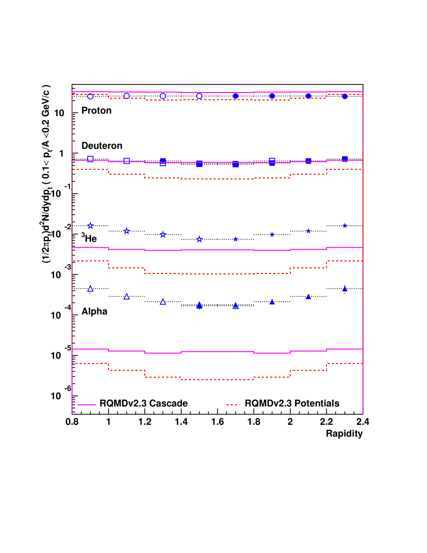
FIG. 19.: Yields measured by E864 near $p_{T}=0$ (in units of $c^{2}/GeV^{2}$) as a function of rapidity for protons (circles), deuterons (squares), ${}^{3}He$ nuclei (stars) and alpha particles (triangles). For comparison, the predictions of the model RQMDv2.3 with a coalescence afterburner are shown for the four species both for RQMD in cascade mode (solid histogram lines) and with mean-field potentials (dashed histogram lines). Hollow symbols represent reflections of E864 data points about midrapidity.

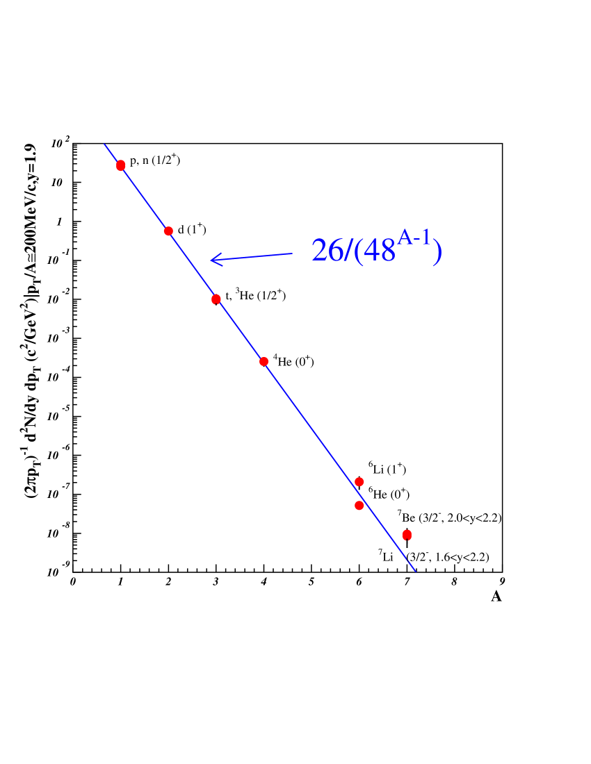
FIG. 20.: Mass dependence of invariant yields of light nuclei from A=1 up to A=7. Yields are measured at $y$=1.9, $p_{T}/A\leq$ 300 MeV/c except where otherwise noted in the plot.

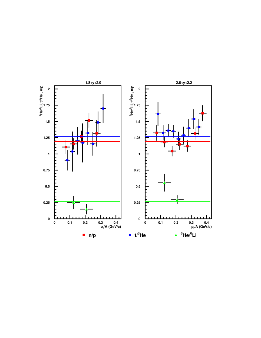
FIG. 21.: $n/p$, $t/^{3}He$, and ${}^{6}He/^{6}Li$ ratios as a function of transverse momentum in two different rapidity slices.

TABLE I.: Summary of experimental conditions under which the light nuclei measurements were made. Events refers to the number (in millions) of sampled events in a given data set.

Year	Field (T)	Trigger	Events (M)	Species	Rapidity	Centrality
1994	+.75	MULT	24	p,d,${}^{3}He$,${}^{4}He$	$1.2\leq y\leq 2.0$	0-10%
1995	+.45	MULT	6	p,d,${}^{3}He$	$1.2\leq y\leq 2.4$	0-10,10-38,38-66%
1996	+1.5	MULT	7	n	$1.6\leq y\leq 3.2$	0-10.10-38,38-66%
1996	+1.5	MULT+LET	13000	${}^{4}He$,${}^{6}He$,${}^{6}Li$, ${}^{7}Li$,${}^{7}Be$	$1.6\leq y\leq 2.2$	10%
1998	+.45	MULT+LET	2000	${}^{4}He$	$1.4\leq y\leq 2.4$	10%

TABLE II.: $B_{A}$ parameters in units of ($GeV^{2}/c^{3})^{(A-1)}$ near collision center-of-mass and source sizes extracted from them from the model of Sato and Yazaki.

A	species	$B_{A}$	$R_{RMS}(fm)$	$y,p_{T}$
2	d	$8.7\pm 1.4\times 10^{-5}$	14.8$\pm$ .7	$1.4\leq y\leq 1.8,\frac{p_{T}}{A}\leq 200MeV$
3	${}^{3}He$	$5.1\pm 1.1\times 10^{-7}$	12.2$\pm$ .5	$1.4\leq y\leq 1.8,\frac{p_{T}}{A}\leq 200MeV$
4	${}^{4}He$	$4.9\pm 1.3\times 10^{-10}$	10.1$\pm$ .3	$1.4\leq y\leq 1.8,\frac{p_{T}}{A}\leq 200MeV$
6	${}^{6}He$	$1.9\pm 0.8\times 10^{-16}$	9.9$\pm$ .3	$1.6\leq y\leq 1.8,\frac{p_{T}}{A}\leq 170MeV$
7	${}^{7}Be$	$1.4\pm 0.7\times 10^{-18}$	9.2$\pm$ .3	$1.6\leq y\leq 2.2,\frac{p_{T}}{A}\leq 250MeV$

TABLE III.: Invariant yields for protons in 10% most central Au+Pb collisions in units of $c^{2}/GeV^{2}$ Errors listed are systematic and statistical combined in quadrature.

Rapidity	1.4-1.6	1.6-1.8	1.8-2.0	2.0-2.2	2.2-2.4	2.4-2.6
$p_{T}$(MeV/c)
25-50	17.9$\pm$ 3.5	22.4$\pm$ 9.6
50-75	28.0$\pm$ 3.5	25.0$\pm$ 2.2	25.2$\pm$ 3.5	14.9$\pm$ 5.1
75-100	26.0$\pm$ 2.2	27.5$\pm$ 2.4	25.8$\pm$ 2.2	26.2$\pm$ 2.5	32.1$\pm$ 6.1
100-125	25.2$\pm$ 3.7	25.9$\pm$ 1.9	27.1$\pm$ 2.0	27.0$\pm$ 2.5	23.3$\pm$ 2.4	20.8$\pm$ 4.3
125-150		26.2$\pm$ 3.0	25.4$\pm$ 1.7	26.2$\pm$ 1.9	24.2$\pm$ 1.9	25.2$\pm$ 2.3
150-175		23.8$\pm$ 6.4	26.4$\pm$ 2.0	27.0$\pm$ 1.9	26.4$\pm$ 1.9	26.1$\pm$ 2.1
175-200			24.6$\pm$ 1.9	24.3$\pm$ 1.8	26.3$\pm$ 1.9	26.5$\pm$ 2.1
200-225			23.4$\pm$ 4.1	25.4$\pm$ 1.9	25.4$\pm$ 1.8	26.0$\pm$ 1.9
225-250			21.1$\pm$ 2.2	24.1$\pm$ 1.9	24.9$\pm$ 1.7	26.2$\pm$ 1.8
250-275			23.8$\pm$ 4.6	23.1$\pm$ 1.7	23.2$\pm$ 1.7	25.5$\pm$ 1.9
275-300				21.9$\pm$ 1.6	23.5$\pm$ 1.9	24.5$\pm$ 1.7
300-325				21.1$\pm$ 2.0	22.3$\pm$ 1.6	22.0$\pm$ 1.6
325-350				20.0$\pm$ 1.6	22.6$\pm$ 1.6	20.7$\pm$ 1.6
350-375				17.6$\pm$ 2.7	22.8$\pm$ 1.7	19.7$\pm$ 1.5
375-400				15.1$\pm$ 2.0	21.3$\pm$ 1.6	19.7$\pm$ 1.5
400-425					21.6$\pm$ 1.6	17.8$\pm$ 1.5
425-450					17.8$\pm$ 1.3	16.3$\pm$ 1.3
450-475					17.8$\pm$ 1.5	16.7$\pm$ 1.4
475-500					17.0$\pm$ 2.5	16.3$\pm$ 1.4
500-525					15.9$\pm$ 1.4	15.3$\pm$ 1.2
525-550						14.4$\pm$ 1.2
550-575						13.5$\pm$ 1.1
575-600						13.5$\pm$ 1.1
600-625						12.0$\pm$ 1.0
625-650						10.0$\pm$ 0.8
650-675						9.2$\pm$ 0.9

TABLE IV.: Invariant yields for protons in 10 to 38% most central Au+Pb collisions in units of $c^{2}/GeV^{2}$ Errors listed are systematic and statistical combined in quadrature.

Rapidity	1.4-1.6	1.6-1.8	1.8-2.0	2.0-2.2	2.2-2.4
$p_{T}$(MeV/c)
25-50	14.3$\pm$ 2.9
50-75	17.9$\pm$ 2.3	17.7$\pm$ 1.6	16.6$\pm$ 2.3	19.1$\pm$ 7.4
75-100	16.5$\pm$ 1.4	16.2$\pm$ 1.4	16.7$\pm$ 1.5	17.7$\pm$ 1.9	20.0$\pm$ 4.2
100-125	16.8$\pm$ 2.5	16.8$\pm$ 1.3	17.3$\pm$ 1.3	19.2$\pm$ 1.8	17.4$\pm$ 1.8
125-150		16.6$\pm$ 1.9	16.8$\pm$ 1.1	16.6$\pm$ 1.2	17.2$\pm$ 1.4
150-175		14.7$\pm$ 4.0	17.2$\pm$ 1.3	17.1$\pm$ 1.2	18.6$\pm$ 1.4
175-200			14.4$\pm$ 1.1	16.3$\pm$ 1.2	18.2$\pm$ 1.4
200-225			14.9$\pm$ 2.6	16.5$\pm$ 1.2	17.1$\pm$ 1.2
225-250			13.8$\pm$ 1.5	15.1$\pm$ 1.2	17.4$\pm$ 1.2
250-275			13.2$\pm$ 2.6	15.3$\pm$ 1.2	15.5$\pm$ 1.1
275-300				14.5$\pm$ 1.1	14.5$\pm$ 1.2
300-325				13.0$\pm$ 1.2	14.5$\pm$ 1.1
325-350				12.1$\pm$ 1.0	14.9$\pm$ 1.1
350-375				11.3$\pm$ 1.8	14.5$\pm$ 1.1
375-400				10.2$\pm$ 1.4	14.2$\pm$ 1.1
400-425					13.8$\pm$ 1.0
425-450					12.1$\pm$ 0.9
450-475					10.4$\pm$ 0.9
475-500					11.1$\pm$ 1.6
500-525					10.3$\pm$ 0.9

TABLE V.: Invariant yields for protons in 38 to 66% most central Au+Pb collisions in units of $c^{2}/GeV^{2}$ Errors listed are systematic and statistical combined in quadrature.

Rapidity	1.4-1.6	1.6-1.8	1.8-2.0	2.0-2.2	2.2-2.4
$p_{T}$(MeV/c)
25-50	4.4$\pm$ 0.9
50-75	6.9$\pm$ 0.9	7.1$\pm$ 0.7	7.5$\pm$ 1.1	7.5$\pm$ 2.9
75-100	6.9$\pm$ 0.7	7.2$\pm$ 0.7	7.4$\pm$ 0.7	7.6$\pm$ 0.8	9.2$\pm$ 2.1
100-125	6.6$\pm$ 1.0	7.0$\pm$ 0.6	7.3$\pm$ 0.6	8.1$\pm$ 0.8	8.0$\pm$ 0.9
125-150		7.3$\pm$ 0.8	7.0$\pm$ 0.5	7.4$\pm$ 0.6	8.3$\pm$ 0.7
150-175		5.6$\pm$ 1.5	7.1$\pm$ 0.6	7.6$\pm$ 0.6	8.9$\pm$ 0.7
175-200			5.7$\pm$ 0.5	6.8$\pm$ 0.5	8.5$\pm$ 0.7
200-225			6.3$\pm$ 1.1	7.1$\pm$ 0.5	8.1$\pm$ 0.6
225-250			5.1$\pm$ 0.6	6.6$\pm$ 0.6	8.0$\pm$ 0.6
250-275			5.8$\pm$ 1.2	6.5$\pm$ 0.5	7.1$\pm$ 0.5
275-300				6.6$\pm$ 0.5	7.0$\pm$ 0.6
300-325				5.7$\pm$ 0.6	6.8$\pm$ 0.5
325-350				5.3$\pm$ 0.5	7.1$\pm$ 0.5
350-375				4.7$\pm$ 0.7	6.5$\pm$ 0.5
375-400				4.3$\pm$ 0.6	6.3$\pm$ 0.5
400-425					6.0$\pm$ 0.5
425-450					5.2$\pm$ 0.4
450-475					4.6$\pm$ 0.4
475-500					4.8$\pm$ 0.7
500-525					3.9$\pm$ 0.4

TABLE VI.: Invariant yields for deuterons in 10% most central Au+Pb collisions in units of $10^{-2}c^{2}/GeV^{2}$ in bins with low transverse momentum (see also the following table for the high transverse momentum data). Errors listed are systematic and statistical combined in quadrature.

Rapidity	1.0-1.2	1.2-1.4	1.4-1.6	1.6-1.8	1.8-2.0	2.0-2.2	2.2-2.4	2.4-2.6
$p_{T}(MeV/c)$
37.5	74.7$\pm$ 35.7
62.5	76.4$\pm$ 8.8	53.7$\pm$ 11.0
87.5	71.2$\pm$ 6.4	63.1$\pm$ 5.8	48.2$\pm$ 6.4	75.9$\pm$ 26.7
112.5	69.3$\pm$ 6.2	61.7$\pm$ 5.3	52.6$\pm$ 5.8	56.1$\pm$ 9.3	43.0$\pm$ 9.7
137.5	72.5$\pm$ 8.6	66.0$\pm$ 5.9	53.9$\pm$ 5.9	56.6$\pm$ 5.2	54.4$\pm$ 5.6	68.1$\pm$ 14.0
162.5	86.6$\pm$ 16.6	59.3$\pm$ 4.7	53.2$\pm$ 4.9	54.4$\pm$ 5.4	56.4$\pm$ 5.2	70.4$\pm$ 6.9	59.1$\pm$ 18.2
187.5		65.1$\pm$ 5.3	58.0$\pm$ 4.6	56.5$\pm$ 5.0	53.5$\pm$ 4.4	64.5$\pm$ 6.0	70.6$\pm$ 8.6
212.5		67.5$\pm$ 7.2	50.1$\pm$ 4.3	54.5$\pm$ 5.2	56.6$\pm$ 4.9	60.5$\pm$ 4.7	71.0$\pm$ 7.0	89.7$\pm$ 13.7
237.5		56.7$\pm$ 8.4	57.3$\pm$ 5.3	59.4$\pm$ 4.6	58.0$\pm$ 4.5	61.6$\pm$ 4.7	66.5$\pm$ 6.2	91.0$\pm$ 9.6
262.5		67.3$\pm$ 14.3	57.2$\pm$ 5.0	59.4$\pm$ 4.7	58.6$\pm$ 4.2	65.1$\pm$ 4.9	72.9$\pm$ 5.9	98.7$\pm$ 8.2
287.5			56.3$\pm$ 5.0	52.1$\pm$ 5.2	58.0$\pm$ 4.2	61.1$\pm$ 4.3	74.0$\pm$ 5.5	86.3$\pm$ 6.8
312.5			50.8$\pm$ 4.7	51.0$\pm$ 4.5	54.5$\pm$ 4.6	64.3$\pm$ 4.3	75.2$\pm$ 5.5	95.1$\pm$ 8.4
337.5			46.3$\pm$ 5.7	55.1$\pm$ 4.5	56.1$\pm$ 4.8	64.6$\pm$ 4.4	72.2$\pm$ 5.1	89.8$\pm$ 9.3
362.5			52.7$\pm$ 8.7	52.0$\pm$ 4.2	54.8$\pm$ 5.5	66.6$\pm$ 4.4	68.4$\pm$ 6.0	85.8$\pm$ 9.1
387.5			44.1$\pm$ 11.3	53.7$\pm$ 4.5	54.2$\pm$ 4.5	68.2$\pm$ 4.9	70.3$\pm$ 5.1	87.2$\pm$ 8.8
412.5				47.8$\pm$ 4.3	55.1$\pm$ 5.0	61.8$\pm$ 4.7	71.3$\pm$ 5.0	82.0$\pm$ 7.8
437.5				51.3$\pm$ 4.4	56.2$\pm$ 4.6	62.0$\pm$ 5.4	75.9$\pm$ 5.2	88.1$\pm$ 9.1
462.5				48.2$\pm$ 5.0	56.5$\pm$ 4.3	58.3$\pm$ 5.1	66.7$\pm$ 4.8	85.7$\pm$ 8.6
487.5				50.8$\pm$ 7.9	57.2$\pm$ 4.4	57.6$\pm$ 4.5	68.2$\pm$ 5.2	82.0$\pm$ 8.8
512.5				46.1$\pm$ 6.4	55.0$\pm$ 4.3	64.4$\pm$ 5.3	65.2$\pm$ 5.2	80.3$\pm$ 7.1
537.5					54.1$\pm$ 4.3	61.1$\pm$ 5.7	59.5$\pm$ 4.7	75.0$\pm$ 8.0

TABLE VII.: Invariant yields for deuterons in 10% most central Au+Pb collisions in units of $10^{-2}c^{2}/GeV^{2}$ in bins with high transverse momentum (see also the previous table for the low transverse momentum data). Errors listed are systematic and statistical combined in quadrature.

Rapidity	1.0-1.2	1.2-1.4	1.4-1.6	1.6-1.8	1.8-2.0	2.0-2.2	2.2-2.4	2.4-2.6
$p_{T}(MeV/c)$
512.5				46.1$\pm$ 6.4	55.0$\pm$ 4.3	64.4$\pm$ 5.3	65.2$\pm$ 5.2	80.3$\pm$ 7.1
537.5					54.1$\pm$ 4.3	61.1$\pm$ 5.7	59.5$\pm$ 4.7	75.0$\pm$ 8.0
562.5					51.7$\pm$ 4.3	61.2$\pm$ 7.7	64.8$\pm$ 5.6	77.1$\pm$ 8.6
587.5					50.2$\pm$ 4.4	64.4$\pm$ 4.9	62.1$\pm$ 5.3	71.1$\pm$ 7.4
612.5					57.6$\pm$ 4.9	63.5$\pm$ 6.1	60.4$\pm$ 5.2	65.9$\pm$ 7.3
637.5					56.3$\pm$ 8.1	55.9$\pm$ 4.2	63.6$\pm$ 5.6	66.6$\pm$ 8.4
662.5					43.6$\pm$ 4.4	61.8$\pm$ 5.6	58.8$\pm$ 5.2	63.7$\pm$ 7.9
687.5					43.0$\pm$ 10.0	55.7$\pm$ 4.4	61.8$\pm$ 5.8	65.7$\pm$ 9.6
712.5						59.5$\pm$ 4.9	58.1$\pm$ 5.1	58.4$\pm$ 8.2
737.5						57.4$\pm$ 4.6	55.8$\pm$ 4.6	58.0$\pm$ 8.2
762.5						60.2$\pm$ 4.5	53.1$\pm$ 4.5	55.4$\pm$ 8.4
787.5						52.6$\pm$ 4.0	53.8$\pm$ 4.2	58.6$\pm$ 9.2
812.5						50.7$\pm$ 6.9	54.3$\pm$ 4.3	55.8$\pm$ 8.2
837.5						49.3$\pm$ 4.2	55.1$\pm$ 4.7	47.6$\pm$ 6.9
862.5						43.3$\pm$ 4.9	52.8$\pm$ 4.4	45.5$\pm$ 5.8
887.5						51.3$\pm$ 7.0	48.4$\pm$ 4.1	50.4$\pm$ 6.7
912.5						47.0$\pm$ 8.4	50.5$\pm$ 4.4	44.4$\pm$ 6.3
937.5							49.4$\pm$ 4.3	42.6$\pm$ 5.3
962.5							45.7$\pm$ 3.8	46.2$\pm$ 6.9
987.5							44.1$\pm$ 3.9	47.6$\pm$ 7.5
1012.5							48.2$\pm$ 4.0	44.2$\pm$ 6.9
1037.5							42.2$\pm$ 4.0	40.7$\pm$ 6.6
1062.5							38.1$\pm$ 3.6	40.6$\pm$ 6.5
1087.5							37.0$\pm$ 4.6	40.9$\pm$ 5.3
1112.5							39.9$\pm$ 4.1	40.7$\pm$ 5.9
1137.5							37.6$\pm$ 4.3	36.8$\pm$ 4.8
1162.5								32.0$\pm$ 4.7
1187.5								31.9$\pm$ 5.1

TABLE VIII.: Invariant yields for deuterons in 10% to 38%most central Au+Pb collisions in units of $10^{-2}c^{2}/GeV^{2}$. Errors listed are systematic and statistical combined in quadrature.

Rapidity	1.0-1.2	1.2-1.4	1.4-1.6	1.6-1.8	1.8-2.0	2.0-2.2	2.2-2.4
$p_{T}(MeV/c)$
25
75	48.2$\pm$ 5.2	42.5$\pm$ 5.5
125	52.4$\pm$ 5.3	40.6$\pm$ 3.8	36.0$\pm$ 4.2	36.1$\pm$ 4.7	35.2$\pm$ 4.9
175		44.9$\pm$ 4.5	33.6$\pm$ 3.6	36.9$\pm$ 3.5	38.1$\pm$ 3.5	42.7$\pm$ 4.6
225		42.8$\pm$ 5.4	34.6$\pm$ 3.3	35.2$\pm$ 3.0	36.4$\pm$ 3.2	38.5$\pm$ 4.0	52.3$\pm$ 4.9
275			38.2$\pm$ 3.7	34.4$\pm$ 3.3	38.5$\pm$ 2.9	45.3$\pm$ 3.5	57.7$\pm$ 4.3
325			33.4$\pm$ 3.7	37.7$\pm$ 3.2	35.5$\pm$ 3.6	41.3$\pm$ 3.4	52.1$\pm$ 4.7
375			31.4$\pm$ 6.9	33.0$\pm$ 3.1	36.2$\pm$ 3.4	42.3$\pm$ 3.2	56.4$\pm$ 4.1
425				29.9$\pm$ 2.9	37.8$\pm$ 3.7	40.9$\pm$ 3.4	53.0$\pm$ 3.9
475				29.4$\pm$ 4.1	35.9$\pm$ 3.1	37.0$\pm$ 3.3	46.8$\pm$ 3.9
525				25.0$\pm$ 5.1	35.7$\pm$ 3.0	36.9$\pm$ 4.6	45.2$\pm$ 4.1
575					31.5$\pm$ 3.1	41.2$\pm$ 3.5	43.3$\pm$ 4.2
625					33.6$\pm$ 3.9	34.2$\pm$ 4.0	43.3$\pm$ 3.8
675					25.8$\pm$ 4.3	39.3$\pm$ 3.3	38.7$\pm$ 3.5
725						33.6$\pm$ 3.2	42.2$\pm$ 3.7
775						33.1$\pm$ 3.6	36.3$\pm$ 3.1
825						27.1$\pm$ 3.5	36.1$\pm$ 3.9
875						28.3$\pm$ 3.6	34.2$\pm$ 3.5
925						29.6$\pm$ 4.2	30.3$\pm$ 3.9
975							25.7$\pm$ 2.4
1025							27.6$\pm$ 2.5
1075							24.0$\pm$ 2.5
1125							22.8$\pm$ 3.1
1175							17.6$\pm$ 2.8

TABLE IX.: Invariant yields for deuterons in 38% to 66%most central Au+Pb collisions in units of $10^{-2}c^{2}/GeV^{2}$. Errors listed are systematic and statistical combined in quadrature.

Rapidity	1.0-1.2	1.2-1.4	1.4-1.6	1.6-1.8	1.8-2.0	2.0-2.2	2.2-2.4
$p_{T}(MeV/c)$
75	22.3$\pm$ 2.8	19.0$\pm$ 2.8
125	23.4$\pm$ 2.8	18.9$\pm$ 2.0	16.4$\pm$ 2.1	12.5$\pm$ 1.9	17.7$\pm$ 2.9
175		15.9$\pm$ 2.0	13.8$\pm$ 1.6	13.5$\pm$ 1.9	12.4$\pm$ 1.7	17.6$\pm$ 2.0
225		18.1$\pm$ 2.9	14.8$\pm$ 1.7	13.0$\pm$ 1.6	14.3$\pm$ 2.1	18.1$\pm$ 1.9	25.4$\pm$ 2.5
275		22.0$\pm$ 7.5	12.7$\pm$ 1.7	12.8$\pm$ 1.7	13.2$\pm$ 1.4	17.3$\pm$ 1.6	26.8$\pm$ 2.3
325			10.3$\pm$ 1.6	14.0$\pm$ 1.8	12.9$\pm$ 1.5	16.8$\pm$ 1.5	24.3$\pm$ 2.1
375			12.4$\pm$ 3.2	12.2$\pm$ 1.7	12.2$\pm$ 1.6	17.1$\pm$ 1.6	23.2$\pm$ 2.0
425				10.6$\pm$ 1.4	13.4$\pm$ 1.5	15.2$\pm$ 1.5	22.7$\pm$ 1.8
475				12.3$\pm$ 2.1	13.6$\pm$ 1.4	17.0$\pm$ 1.6	20.8$\pm$ 1.8
525				9.2$\pm$ 2.4	13.5$\pm$ 1.4	15.2$\pm$ 1.5	19.1$\pm$ 2.2
575					11.8$\pm$ 1.3	14.7$\pm$ 1.9	17.6$\pm$ 1.8
625					16.6$\pm$ 2.2	14.4$\pm$ 1.5	19.6$\pm$ 1.9
675					14.0$\pm$ 2.6	15.1$\pm$ 1.5	16.2$\pm$ 1.9
725						13.0$\pm$ 1.4	14.4$\pm$ 2.4
775						12.0$\pm$ 1.3	12.8$\pm$ 1.9
825						11.7$\pm$ 1.5	12.7$\pm$ 1.4
875						9.7$\pm$ 1.5	12.1$\pm$ 1.9
925							10.4$\pm$ 2.0
975							7.9$\pm$ 1.4
1025							9.0$\pm$ 1.5
1075							7.9$\pm$ 1.6
1125							7.5$\pm$ 1.1

TABLE X.: Invariant yields for ${}^{3}He$ in 10% most central Au+Pb collisions in units of $10^{-3}c^{2}/GeV^{2}$. Errors listed are systematic and statistical combined in quadrature.

Rapidity	1.0-1.2	1.2-1.4	1.4-1.6	1.6-1.8	1.8-2.0	2.0-2.2	2.2-2.4	2.4-2.6
$p_{T}(MeV/c)$
150	8.6$\pm$ 1.6	7.9$\pm$ 1.0	6.7$\pm$ 1.0	8.6$\pm$ 1.7	8.0$\pm$ 2.9
250	9.9$\pm$ 4.4	8.1$\pm$ 1.0	7.4$\pm$ 0.7	8.4$\pm$ 0.8	10.3$\pm$ 1.1	9.8$\pm$ 1.3	15.7$\pm$ 3.8
350			8.4$\pm$ 1.0	7.4$\pm$ 0.7	10.1$\pm$ 0.8	12.1$\pm$ 1.1	15.8$\pm$ 1.5	22.2$\pm$ 3.2
450			5.6$\pm$ 1.6	8.3$\pm$ 0.9	9.7$\pm$ 0.8	11.7$\pm$ 1.0	16.8$\pm$ 1.3	19.1$\pm$ 1.8
550				6.6$\pm$ 0.8	8.9$\pm$ 0.9	11.7$\pm$ 0.9	15.6$\pm$ 1.2	21.6$\pm$ 1.8
650				7.6$\pm$ 1.4	8.6$\pm$ 0.9	12.4$\pm$ 1.0	14.3$\pm$ 1.1	21.9$\pm$ 1.8
750					8.0$\pm$ 0.9	11.5$\pm$ 1.0	14.0$\pm$ 1.1	19.2$\pm$ 1.6
850					7.2$\pm$ 0.9	11.9$\pm$ 1.2	14.7$\pm$ 1.3	17.2$\pm$ 1.6
950					6.6$\pm$ 1.4	9.2$\pm$ 0.9	11.8$\pm$ 1.1	15.7$\pm$ 1.7
1050						9.1$\pm$ 0.9	12.7$\pm$ 1.1	13.9$\pm$ 1.7
1150						10.2$\pm$ 1.1	10.9$\pm$ 1.0	12.9$\pm$ 1.6
1250						8.1$\pm$ 1.3	9.9$\pm$ 0.9	11.2$\pm$ 1.3
1350						6.3$\pm$ 1.2	10.8$\pm$ 1.0	9.6$\pm$ 1.1
1450							9.3$\pm$ 0.9	9.8$\pm$ 1.0
1550							6.5$\pm$ 0.8	7.9$\pm$ 0.9
1650							5.4$\pm$ 0.9	6.1$\pm$ 0.8
1750							5.0$\pm$ 0.9	5.7$\pm$ 0.7
1850								4.4$\pm$ 0.6
1950								3.2$\pm$ 0.5
2050								2.6$\pm$ 0.4

TABLE XI.: Invariant yields for ${}^{3}He$ in 10% to 38% most central Au+Pb collisions in units of $10^{-3}c^{2}/GeV^{2}$. Errors listed are systematic and statistical combined in quadrature.

Rapidity	1.0-1.2	1.2-1.4	1.4-1.6	1.6-1.8	1.8-2.0	2.0-2.2	2.2-2.4
$p_{T}(MeV/c)$
100	8.2$\pm$ 3.0	6.4$\pm$ 2.3	6.0$\pm$ 1.8	6.2$\pm$ 2.6
300		6.2$\pm$ 1.8	5.8$\pm$ 1.0	4.5$\pm$ 0.7	5.8$\pm$ 0.9	9.8$\pm$ 1.3	11.9$\pm$ 2.0
500				4.2$\pm$ 0.9	3.9$\pm$ 0.6	8.2$\pm$ 0.9	13.2$\pm$ 1.2
700				4.9$\pm$ 1.8	5.0$\pm$ 1.0	7.8$\pm$ 1.0	11.1$\pm$ 1.0
900					3.7$\pm$ 1.0	8.8$\pm$ 1.1	7.7$\pm$ 1.0
1100						5.4$\pm$ 0.9	7.8$\pm$ 0.9
1300						2.9$\pm$ 0.9	6.7$\pm$ 0.8
1500							3.9$\pm$ 0.8

TABLE XII.: Invariant yields for ${}^{3}He$ in 38% to 66% most central Au+Pb collisions in units of $10^{-3}c^{2}/GeV^{2}$. Errors listed are systematic and statistical combined in quadrature.

Rapidity	1.0-1.2	1.2-1.4	1.4-1.6	1.6-1.8	1.8-2.0	2.0-2.2	2.2-2.4
$p_{T}(MeV/c)$
100	4.8$\pm$ 2.3	1.9$\pm$ 0.9	2.4$\pm$ 1.0
300			2.5$\pm$ 0.6	1.9$\pm$ 0.4	2.3$\pm$ 0.5	2.9$\pm$ 0.6	7.0$\pm$ 1.4
500				1.5$\pm$ 0.5	2.5$\pm$ 0.5	2.9$\pm$ 0.4	5.2$\pm$ 0.6
700					2.5$\pm$ 0.6	2.2$\pm$ 0.4	4.4$\pm$ 0.5
900					1.4$\pm$ 0.6	2.7$\pm$ 0.5	3.6$\pm$ 0.6
1100						1.7$\pm$ 0.5	3.5$\pm$ 0.6
1300							2.4$\pm$ 0.5
1500							1.7$\pm$ 0.4

TABLE XIII.: Invariant yields for tritons in 10% most central Au+Pb collisions in units of $10^{-3}c^{2}/GeV^{2}$. Errors listed are systematic and statistical combined in quadrature.

Rapidity	1.0-1.2	1.2-1.4	1.4-1.6	1.6-1.8	1.8-2.0	2.0-2.2	2.2-2.4
$p_{T}$
50	12.5$\pm$ 3.6
150	16.0$\pm$ 1.8	11.8$\pm$ 1.5	9.8$\pm$ 1.5
250	13.6$\pm$ 1.9	12.2$\pm$ 1.5	9.9$\pm$ 2.1	11.8$\pm$ 2.9	9.3$\pm$ 1.3	15.9$\pm$ 2.5
350		13.6$\pm$ 1.7	9.6$\pm$ 1.5	12.2$\pm$ 2.4	10.4$\pm$ 3.2	16.0$\pm$ 1.8	16.1$\pm$ 2.4
450		9.2$\pm$ 2.4	10.2$\pm$ 1.5	10.1$\pm$ 1.7	11.7$\pm$ 2.5	16.0$\pm$ 1.7	18.5$\pm$ 2.1
550			10.6$\pm$ 1.4	10.0$\pm$ 1.5	10.5$\pm$ 3.1	15.8$\pm$ 1.6	18.7$\pm$ 1.9
650				9.0$\pm$ 1.1	11.4$\pm$ 2.0	15.3$\pm$ 1.7	17.5$\pm$ 2.0
750				10.5$\pm$ 1.5	9.3$\pm$ 1.6	14.8$\pm$ 1.9	17.0$\pm$ 1.9
850					10.7$\pm$ 1.5	16.7$\pm$ 2.2	14.8$\pm$ 2.0
950					11.2$\pm$ 1.3	14.1$\pm$ 2.0	13.9$\pm$ 2.5
1050						12.9$\pm$ 1.4	15.7$\pm$ 1.8
1150							12.2$\pm$ 2.0
1250							14.3$\pm$ 1.9
1350							9.1$\pm$ 1.2
1450							9.7$\pm$ 1.3

TABLE XIV.: Invariant yields for ${}^{4}He$ in 10% most central Au+Pt collisions in units of $10^{-5}c^{2}/GeV^{2}$ from data taken in the 1998 run of E864. Errors listed are systematic and statistical combined in quadrature.

Rapidity	1.4-1.6	1.6-1.8	1.8-2.0	2.0-2.2	2.2-2.4
$p_{T}(MeV/c)$
350	17.3$\pm$ 1.9	17.4$\pm$ 2.0	22.1$\pm$ 2.6
450	18.1$\pm$ 2.4	16.7$\pm$ 1.7	23.3$\pm$ 2.5	26.0$\pm$ 3.1
550	17.4$\pm$ 2.4	20.3$\pm$ 2.6	19.4$\pm$ 1.9	28.0$\pm$ 3.3	43.7$\pm$ 11.4
650	13.4$\pm$ 2.1	18.0$\pm$ 2.2	21.7$\pm$ 2.3	30.5$\pm$ 3.5	44.5$\pm$ 11.3
750	20.4$\pm$ 5.4	17.2$\pm$ 2.3	21.1$\pm$ 2.4	29.8$\pm$ 3.5	45.6$\pm$ 11.4
850		16.9$\pm$ 2.3	21.2$\pm$ 2.3	31.7$\pm$ 3.8	47.1$\pm$ 11.8
950		17.9$\pm$ 2.8	20.3$\pm$ 2.2	28.9$\pm$ 3.5	45.8$\pm$ 11.4
1050		15.5$\pm$ 3.0	23.6$\pm$ 2.8	27.6$\pm$ 3.5	42.3$\pm$ 10.6
1150			19.8$\pm$ 2.3	27.1$\pm$ 3.4	38.5$\pm$ 9.7
1250			18.7$\pm$ 2.3	27.6$\pm$ 3.4	41.6$\pm$ 10.6
1350			23.4$\pm$ 4.0	23.9$\pm$ 3.0	37.0$\pm$ 9.5
1450				25.8$\pm$ 3.3	32.0$\pm$ 8.4
1550				21.1$\pm$ 2.8	30.7$\pm$ 8.1
1650				22.3$\pm$ 3.3	29.1$\pm$ 7.6
1750				20.8$\pm$ 3.5	21.5$\pm$ 5.8
1850				15.3$\pm$ 2.7	21.2$\pm$ 5.7
1950					18.5$\pm$ 5.1
2050					13.4$\pm$ 3.9
2150					16.5$\pm$ 5.2

TABLE XV.: Invariant yields for ${}^{6}He$ and ${}^{6}Li$ in Au+Pt collisions in units of $10^{-8}c^{2}/GeV^{2}$. Errors listed are systematic and statistical combined in quadrature.

($y,p_{T}(MeV/c)$)	${}^{6}He$	${}^{6}Li$
(1.6-1.8,500-1000)	6.0 $\pm$ 1.8
(1.8-2.0,0-500)	10.5 $\pm$ 4.6
(1.8-2.0,500-1000)	5.2 $\pm$ 1.2	32 $\pm$ 15
(1.8-2.0,1000-1500)	3.3 $\pm$ 1.2	24.9 $\pm$ 6.1
(2.0-2.2,500-1000)	13.8 $\pm$ 1.2	33.7 $\pm$ 6.9
(2.0-2.2,1000-1500)	10.4 $\pm$ 1.2	37.5 $\pm$ 7.8
(2.0-2.2,1500-2000)		34 $\pm$ 21

TABLE XVI.: Invariant yields for ${}^{7}Li$ and ${}^{7}Be$ in Au+Pt collisions in units of $10^{-8}c^{2}/GeV^{2}$. Errors listed are systematic and statistical combined in quadrature.

($y,p_{T}(GeV/c)$)	${}^{7}Li$	${}^{7}Be$
(1.6-2.2,0-1.8)	.92 $\pm$ .4
(2.0-2.2,0-1.8)		1.3 $\pm^{.35}_{.25}$

REFERENCES

- [1] Present address: Vanderbilt University, Nashville, Tennessee 37235
- [2] Present Address: Istituto di Cosmo-Geofisica del CNR, Torino, Italy / INFN Torino, Italy
- [3] Present Address: Anderson Consulting, Hartford, CT
- [4] Present address: Univ. of Denver, Denver CO 80208
- [5] Deceased.
- [6] Present address: Cambridge Systematics, Cambridge, MA 02139
- [7] Present address: McKinsey & Co., New York, NY 10022
- [8] Present address: Department of Radiation Oncology, Medical College of Virginia, Richmond VA 23298
- [9] Present address: University of Tennessee, Knoxville TN 37996
- [10] Present address: Institut de Physique Nucléaire, 91406 Orsay Cedex, France
- [11] Present Address: Institute for Defense Analysis, Alexandria VA 22311
- [12] Present Address: MIT Lincoln Laboratory, Lexington MA 02420-9185
- [13] S. Pratt, Phys. Rev. Lett. 53(1984)1219.
- [14] L. C. Alexa et. al., Phys. Rev. Lett. 82(1999) 1374. D. Abbott et al., Phys. Rev. Lett. 82(1999) 1379.
- [15] S.C. Johnson, PhD Thesis, SUNY Stony Brook 1997.
- [16] H. Sato and K. Yazaki, Phys. Lett. B 98(1981) 153.
- [17] R. Bond, P.J. Johansen, S.E. Koonin, and S. Garpman, Phys. Lett. B 72(1981) 131.
- [18] J.L. Nagle, B.S. Kumar, D. Kusnezov , H. Sorge and R. Matiello, Phys. Rev. C 53(1996) 367.
- [19] G. Ambrosini et. al., Nucl. Phys. A610(1996) 306.
- [20] P. Braun-Munzinger, J. Stachel, J.P. Wessels, and N. Xu, Phys. Lett. B 344(1995) 43.
- [21] H.Dobler, J.Sollfrank, and U. Heinz Phys. Lett. B 457(1999) 353.
- [22] H. Sorge, A. von Keitz, R. Matiello, H. Stocker, and W. Greiner, Nucl. Phys. A525(1991) 95c.
- [23] R. Scheibl and U. Heinz, Phys. Rev. C. 59(1999)1585.
- [24] A. Polleri, J.P. Bondorf, and I.N. Mishustin, Phys. Lett. B 419(1998) 19.
- [25] S. Das Gupta and A.Z. Mekjian, Phys. Rep. C 53(1996) 367.
- [26] P. Braun-Munzinger, J. Stachel, J.P. Wessels, and N. Xu, Phys. Lett. B 365(1996) 1.
- [27] S. Nagamiya et. al., Phys. Rev. C 24(1981) 971.
- [28] M.J. Bennett et. al., Phys. Rev. C. 58(1998)1155.
- [29] T. Abbott et. al., Phys. Rev. C 50(1994) 1024.
- [30] T. A. Armstrong et al., Nucl. Inst. Meth. A437(1999)222.
- [31] P. Haridas, I.A. Pless. G. Van Buren, J. Tomasi, M.S.Z. Rabin, K. Barish and R.D. Majka, Nucl. Inst. Meth. A385(1997) 413.
- [32] A. Chikanian, B.S. Kumar, N. Smirnov and E.O’Brien, Nucl. Inst. Meth. A371(1996) 480.
- [33] T.A. Armstrong et. al., Nucl. Inst. Meth. A406(1998)227.
- [34] J.C. Hill et. al., Nucl. Inst. Meth. A421(1999)431.
- [35] T.A. Armstrong et. al., Phys. Rev. C 60(1999)064903.
- [36] Ph.D. theses: N.K. George, Z. Xu, S.D. Coe, J.K. Pope, L.E. Finch (Yale University) ,R. Hoversten (Iowa State University, in preparation).
- [37] S. Ahmad et. al., Phys. Lett. B 382(1996) 35.
- [38] J. Barrette et. al., nucl-ex/9906005.
- [39] N.K. George, Talk presented at Park City Utah, January 9-16, 1999. Proceedings to be published by Kluwer Academic Press, 1999.
- [40] T.A. Armstrong et. al., Phys. Rev. C 59(1999) 2699.
- [41] W.J. Llope et.al., Phys. Rev. C 52(1995) 2004.
- [42] M. Murray for the NA44 Collaboration, ICPAQGP 97 Conference.; nucl-ex/9706007.
- [43] R. Mattiello, H.Sorge, H.Stocker, and W. Griener, Phys. Rev. C. 55(1997)1443.
- [44] S. Wang et. al., Phys. Rev. Lett. 74(1995) 2646.
- [45] Z. Xu for the E864 Collaboration, ISMD 99 Conference.; nucl-ex/9909012.
- [46] T.A. Armstrong et al., Phys. Rev. Lett. 83(1999) 5431.