Universal shape law of stochastic supercritical bifurcations: Theory and experiments.

Abstract

A universal law for the supercritical bifurcation shape of transverse one-dimensional (1D) systems in presence of additive noise is given. The stochastic Langevin equation of such systems is solved by using a Fokker-Planck equation leading to the expression for the most probable amplitude of the critical mode. From this universal expression, the shape of the bifurcation, its location and its evolution with the noise level are completely defined. Experimental results obtained for a 1D transverse Kerr-like slice subjected to optical feedback are in excellent agreement.

In nature, most of physical systems are subjected to fluctuations. For a long time, the effects of these fluctuations were either considered as a nuisance (degradation of the signal-to-noise ratio) or ignored because it was not known how to handle them. Since three decades, a wealth of theoretical and experimental researches have shown that fluctuations can have rather surprisingly constructive and counterintuitive effects in many physical systems and that they can be figured out with the help of different analysis tools. These situations occur when there are mechanisms of noise amplification or when noise interacts with nonlinearities or driving forces on the system. The most well-know examples in zero dimensional systems are noise induced transition HL84 and stochastic resonance GHJM98 . More recently, examples in spatially extended system are noise induced phase transition, noise-induced patterns (see OS99 and references therein), noise-sustained structures in convective instability AGTL06 , stochastic spatio-temporal intermittency SanMiguiel , noise-induced travelling waves Zhou , noise-induced ordering transition MLKB97 and front propagation ClercNoise2006 . A direct consequence of noise effects is the modification of the deterministic bifurcation shapes. The critical points and the physical mechanisms are masked by fluctuations. It is important to remark that the critical points generically represent a change of balance between forces. Hence, the characterization of noisy bifurcations is a fundamental problem due to the ubiquitous nature of bifurcations. For instance, the supercritical bifurcations transform into smooth transitions between the two states and the subcritical bifurcations experience hysteresis size modifications. In absence of noise, the shape of a bifurcation and its characteristics are given by the analytical solution of the deterministic amplitude equation of the critical mode CrossHohenberg . On the other hand, in presence of noise, no such analytical expression can be obtained from the stochastic amplitude equation. In this latter situation, the below and above bifurcation point regimes can be treated separately, but without continuity between their respective solutions. For instance, in noisy spatially extended systems in which the systems are characterized by the appearance of pattern precursors below the bifurcation point and by established patterns that fluctuate above this point Gonzague , the precursor amplitude SZ93 , obtained from the linear study of the stochastic equation, diverges at the bifurcation point and does not connect to the “mean” amplitude of the fluctuating pattern, obtained from the deterministic equation. To our knowledge, no universal analytical expression of the critical mode amplitude, describing the complete transition from below to above the bifurcation point, exists for the supercritical bifurcations in presence of noise.

In this letter, we propose a universal description of the supercritical bifurcation shapes of 1D transverse systems (either uniforms or very slowly varying in space) in presence of noise that is also valid for the second order bifurcations of temporal (zero-dimensional) systems. More precisely, we give a unified expression for the most probable amplitude describing the supercritical bifurcations in presence of noise, including the noise level and the bifurcation point location. The systems under study are described by stochastic partial differential equations of the Langevin type VanKampen (first order in time and with linear noise terms) involving additive white noise. Firstly, we solve the Langevin equation describing the stochastic dynamics by using a Fokker-Planck equation for the probability density of the critical mode amplitude. Then, from the stationary distribution of this amplitude, we deduce the bifurcation shape by means of the most probable value of the pattern amplitude. Finally, the comparison with experimental results obtained in a Kerr-like slice subjected to 1D optical feedback is given and leads to an excellent agreement.

Let us consider a 1D extended system that exhibits a supercritical spatial bifurcation described by

$$\partial_{t}\vec{u}=\vec{f}(\vec{u},\partial_{x},\left\{\mu\right\})+\sqrt{\eta}\vec{\zeta}(x,t)$$ (1)

where $\vec{u}\left(x,t\right)$ is a field that describes the system under study, $\vec{f}$ is the vector field, $\left\{\mu\right\}$ is a set of parameters that characterizes the system, $\eta$ is the noise level intensity, and $\vec{\zeta}(x,t)$ is a white Gaussian noise with zero mean value and correlation $\left\langle\zeta^{i}(x,t)\zeta^{j}(x{\acute{}},t{\acute{}})\right\rangle=\delta^{ij}\delta\left(t{\acute{}}-t\right)\delta\left(x{\acute{}}-x\right)$.

We assume that the associated deterministic system ($\eta=0$) possesses a stationary state $\vec{u}_{0}$, that satisfies $\vec{f}(\vec{u}_{o},\partial_{x},\left\{\mu\right\})=0$. Above a set of critical values $\left\{\mu_{c}\right\}$, the system exhibits a spatial instability such that $\vec{u}$ reads $\vec{u}\left(x,t\right)=\vec{u}_{0}+e^{\lambda(k)t+ikx}\hat{u},$ where $\lambda\left(k\right)$ is the linear growth rate and $k$ the wave number of the instability. Close to $\left\{\mu_{c}\right\}$, for $\lambda\left(k\right)<0$ (i.e. $\vec{u}_{0}$ is stable), the profile of $\lambda$ already displays a maximum for a non null wave number close to the critical one $k_{c}$. Hence, below the bifurcation point, when noise is present, among all the excited spatial modes, the one associated with the maximum growth rate ($k\simeq k_{c}$) rules the dynamics. The dynamical behavior of the system is then characterized by pattern precursors. Figure 1 illustrates this property. It shows the instantaneous $S\left(k,t\right)$ and the averaged $S\left(k\right)=<S(k,t)>_{t}$ modulus of the Fourier transform of the field $\vec{u}$, also called the structure factor, for the supercritical Swift-Hohenberg equation OS99 below the deterministic threshold. We can remark that the maxima of the function, both instantaneous and averaged, already give the incoming critical wave numbers $k_{c}=\pm 1$ (Fig.1).

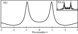
Figure 1: Averaged Fourier transform modulus $S(k)$ of the field $\vec{u}$ for the supercritical Swift-Hohenberg model OS99 obtained below the bifurcation point. The inset figure corresponds to an instantaneous snapshot of $S(k,t)$.

To capture the dynamics of the system of Eq. (1) in an unified description close to the instability threshold, we introduce the ansatz $\vec{u}\left(x,t\right)=\vec{u}_{o}+A\left(T=\varepsilon t,X=\sqrt{\varepsilon}x\right)e^{ik_{c}x}\hat{u}_{k}+\bar{A}\left(T,X\right)e^{-ik_{c}x}\hat{u}_{k}+h.o.t$ CrossHohenberg , where $A$ is the amplitude of critical mode, $\varepsilon$ is the bifurcation parameter which is proportional to $\left\|\mu-\mu_{c}\right\|$, $\hat{u}_{k}$ is the eigenvector associated to the critical mode, $\left\{T,X\right\}$ are the slow time and spatial variables and the high order terms ($h.o.t$) are a series in the amplitude $A$. Introducing the above ansatz in Eq. (1) leads to the amplitude equation that satisfies the solvability condition CrossHohenberg

$$\partial_{T}A=\varepsilon A-|A|^{2}A+\partial_{XX}A+\sqrt{\eta}\xi\left(X,T\right),$$ (2)

where $\xi\left(X,T\right)$ is a white Gaussian noise with null mean value and correlation $\left\langle\xi\left(X,T\right)\xi\left(X^{\prime},T^{\prime}\right)\right\rangle=0$ and $\left\langle\xi\left(X,T\right)\bar{\xi}\left(X^{\prime},T^{\prime}\right)\right\rangle=\delta\left(T{\acute{}}-T\right)\delta\left(X{\acute{}}-X\right)$. The $\xi\left(X,T\right)$ term is then a linear combination of the original noise source term $\vec{\zeta}(x,t)$. In absence of noise ($\eta=0$), when the bifurcation parameter $\mathcal{\varepsilon}$ is negative, the system is characterized by a stable equilibrium state of amplitude $A=0$, and when $\mathcal{\varepsilon}$ becomes positive, the system exhibits a degenerate pitchfork bifurcation whose amplitude evolves as $|A|\sim\sqrt{\varepsilon}$ (deterministic value in Fig. 2).

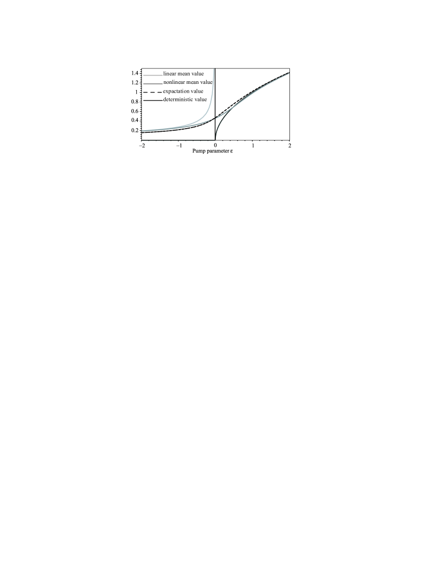
Figure 2: Bifurcation diagrams of the amplitude of the critical mode obtained for different solutions of Eq. (2). Namely, the deterministic value A, the expectation value $|a_{max}|$, the linear and non-linear mean values $\langle|a|\rangle_{linear}$ and $\langle|a|\rangle_{nonlinear}$ respectively (see text for value definitions).

The next step is to consider the global amplitude $a\left(T\right)=\int_{-L/2}^{L/2}A(T,X)dX/L,$ where $L$ is the size of the transverse domain under study. This quantity is relevant to describe the bifurcation as soon as the transverse domain is either uniform or with very slow spatial variations of the control parameters. Experimentally, it will be achieved by choosing a restricted part $L$ of the transverse pattern within which the control parameters are slowly varying. This restriction excludes all specific cases with fast spatial variations (e.g. local structures), which require specific analyses associated with the considered transverse profiles, but they are out of the scope of this paper. The global amplitude $a\left(T\right)$ then satisfies the Langevin equation

$$\partial_{T}a=\varepsilon a-|a|^{2}a+\sqrt{\eta}\varsigma\left(T\right),$$ (3)

where $\varsigma\left(T\right)\equiv\int_{-L/2}^{L/2}\xi(T,X)dX/L$ is a Gaussian white noise with zero expectation value and correlation $\left\langle\varsigma\left(T\right)\bar{\varsigma}\left(T^{\prime}\right)\right\rangle=\delta\left(T{\acute{}}-T\right).$ The general way of obtaining a solution of such Langevin equation is by use of a Fokker-Planck equation which provides us with a deterministic equation satisfied by the time dependent probability density $P(a,\bar{a};T)$ of the amplitude $a$ VanKampen that reads

$$\partial_{T}P=\partial_{a}\left\{-\varepsilon a+|a|^{2}a+\frac{\eta}{2}\partial_{\bar{a}}\right\}P+c.c.$$ (4)

where $c.c.$ means "complex conjugate". The associated stationary probability density of the modulus of a is

$$P_{s}\left(|a|,\varepsilon,\eta\right)=Q(\varepsilon,\eta)|a|e^{\frac{\varepsilon|a|^{2}-\frac{|a|^{4}}{2}}{\eta}},$$ (5)

where $Q(\varepsilon,\eta)\equiv 2\sqrt{2}e^{-\frac{\varepsilon^{2}}{2\eta}}/erfc(-\frac{\varepsilon}{\sqrt{2\eta}})\sqrt{\pi\eta}$. The stationary probability density is shown in Fig. 3 for different values of the bifurcation parameter $\varepsilon$. The probability density function is not symmetrical with respect to its maximum so that the most relevant quantity for characterizing $P_{s}\left(|a|,\varepsilon,\eta\right)$ is its maximum and not its mean value as usually calculated e.g. in experiments. The value of $|a|$ corresponding to the maximum of $P_{s}\left(|a|,\varepsilon,\eta\right)$ occurs at the expectation value $|a_{max}|$ given by

$$|a_{max}|=\sqrt{\frac{\varepsilon+\sqrt{\varepsilon^{2}+2\eta}}{2}}$$ (6)

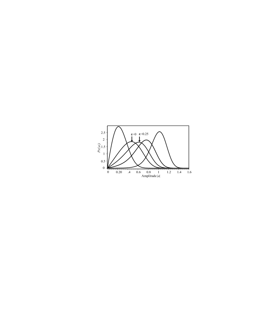
Figure 3: Stationary probability distribution $P_{s}\left(|a|\right)$ for different values of the bifurcation parameter $\varepsilon$. From left to right: $\varepsilon=-1;0;0.25;0.5;1$. $\eta=0.2$.

When the bifurcation parameter $\varepsilon$ is driven far from 0 ($|\varepsilon|\gg 1$), this expectation value converge to zero ($\sqrt{-\eta/2\varepsilon}$) for negative values of $\varepsilon$ and to $\sqrt{\varepsilon}$ (as for the deterministic case) for positive values. Plotting this quantity versus $\varepsilon$ gives the supercritical bifurcation shape in presence of noise (dashed line in Fig. 2). Let’s now discuss the relevance of $|a_{max}|$ for describing the noisy supercritical bifurcation. If we neglect the nonlinear term in the Langevin equation (3), one can perform a linear stability analysis that provides us with the linear mean value of the amplitude modulus $\left\langle|a|\right\rangle_{linear}=\sqrt{-\pi\eta/4\varepsilon}$. Note that this value diverges at the bifurcation point and is only valid for $\varepsilon<0$ (Fig. 2). The corresponding nonlinear mean value $\left\langle|a|\right\rangle_{nonlinear}$ is computed numerically from the probability density $P_{s}(|a|)$. All the linear mean, non-linear mean, expected and deterministic values of the critical mode amplitude are reported on Fig. 2 for comparison. The interesting region is located in the vicinity of the bifurcation point where the behaviors of the different curves strongly differ. The linear mean value and the deterministic value do not correspond to a realistic physical behavior since the amplitude never diverges at threshold and we are considering a noisy system respectively. Only the nonlinear mean and expected values can mimic the supercritical bifurcation in presence of noise. However, as we have mentioned earlier, due to the asymmetry of $P_{s}\left(|a|,\varepsilon,\eta\right)$, the most relevant value for describing the evolution of the amplitude versus the control parameter is the expectation value $|a_{max}|$. As this value includes the noise level $\eta$, we have performed numerical simulations including noise to study the influence of noise on the bifurcation shape. Figure 4 clearly depicts the continuous deformation and evolution of the bifurcation shape with the level of noise. It also shows the very good agreement between the numerical values of $|a_{max}|$ obtained from the numerical simulations of the stochastic supercritical Swift-Hohenberg equation SwiftHohenberg and its analytical value [Eq. (6)]. Thus, the expression of $|a_{max}|$ is the relevant quantity for describing the noisy supercritical bifurcations including the noise level and the bifurcation point location ($\varepsilon=0$) of systems satisfying the Eq. (1).

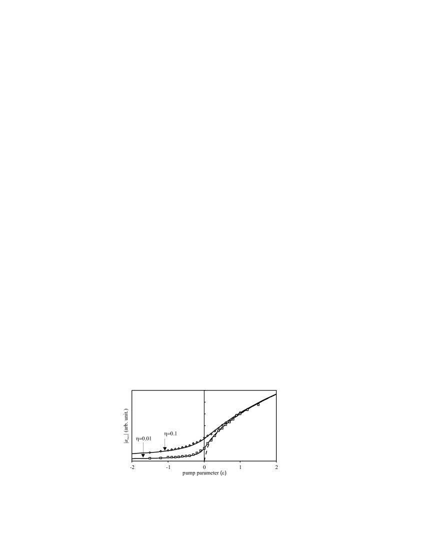
Figure 4: Influence of the noise level $\eta$ on the shape of the unperfect supercritical bifurcation. The continuous curves correspond to the analytical expectation value $|a_{max}|$ of Eq. (6). The squares and losanges are obtained from the numerical simulations of the stochastic Swift-Hohenberg equation Eq. (3).

Regardless of the sign of $\varepsilon$, the width of the stationary probability distribution decreases as $|\varepsilon|$ increases far from 0 (Fig. 3). Therefore, close to the bifurcation point ($\varepsilon=0$) the value of $P_{s}\left(|a_{max}|\right)$ exhibits a minimum versus $\varepsilon$ ($\varepsilon\approx 0.25$ in the case of Fig. 3) which is shifted from this bifurcation point. The width of the stationary probability density is then maximum corresponding to a dynamics characterized by large amplitude fluctuations. This shift between the minimum of $P_{s}\left(|a_{max}|\right)$ and the bifurcation point ($\varepsilon=0$) reminds the bifurcation postponements as in LT86 . After a straightforward calculation, the value of the bifurcation parameter ($\varepsilon_{min}$) associated with the minimum of $P_{s}\left(|a_{max}|\right)$, for a given value of noise intensity, is

$$\varepsilon_{min}\left(\eta\right)\approx 0.55\sqrt{\eta}.$$

It allow us to propose a criterion for the localization of the bifurcation point: for a given noise intensity ($\eta$) the bifurcation point is localized at $\varepsilon_{min}-0.55\sqrt{\eta}$, where $\varepsilon_{min}$ is the value of the control parameter for which $P_{s}\left(|a_{max}|,\varepsilon\right)$ is minimum.

In order to completely validate the universal law of Eq. (6), we have applied our analysis to experiments realized on a noisy 1D transverse system known to exhibit a supercritical bifurcation at the onset of roll pattern formation. The system is a nematic liquid crystal slice subjected to optical feedback (cf. Fig. 5) based on the well known feedback optical system akhman88 ; firth90 . The corresponding stochastic model reads AGTL06

$$\partial_{t}\vec{u}=\left(\partial_{xx}-1\right)\vec{u}+\left|F\right|^{2}+R\left|e^{i\sigma\partial_{xx}}\left(e^{i\chi\vec{u}}F\right)\right|^{2}+\sqrt{\eta}\vec{\zeta}$$ (7)

where $\vec{u}(x,t)$ stands for the refractive index of the nonlinear nematic liquid crystal (LC) layer; $t$ and $x$ are the time and transverse space variables scaled with respect to the relaxation time $\tau$ and the diffusion length $l_{d}$; $R$ is the mirror intensity reflectivity. $\sigma=d/k_{0}$ where $d$ is the slice-mirror distance and $k_{0}$ is the optical wave number of the field. $F$ is the forward input optical field, its transverse profile is accounted for using $F(x)=F_{0}\exp(-x^{2}/w^{2})$ for a Gaussian pump beam of radius $w$. $\zeta$ and $\eta$ are the noise source and level respectively as defined in Eq. (1). The Kerr effect is parametrized by $\chi$ which is positive (negative) for a focusing (defocusing) medium.

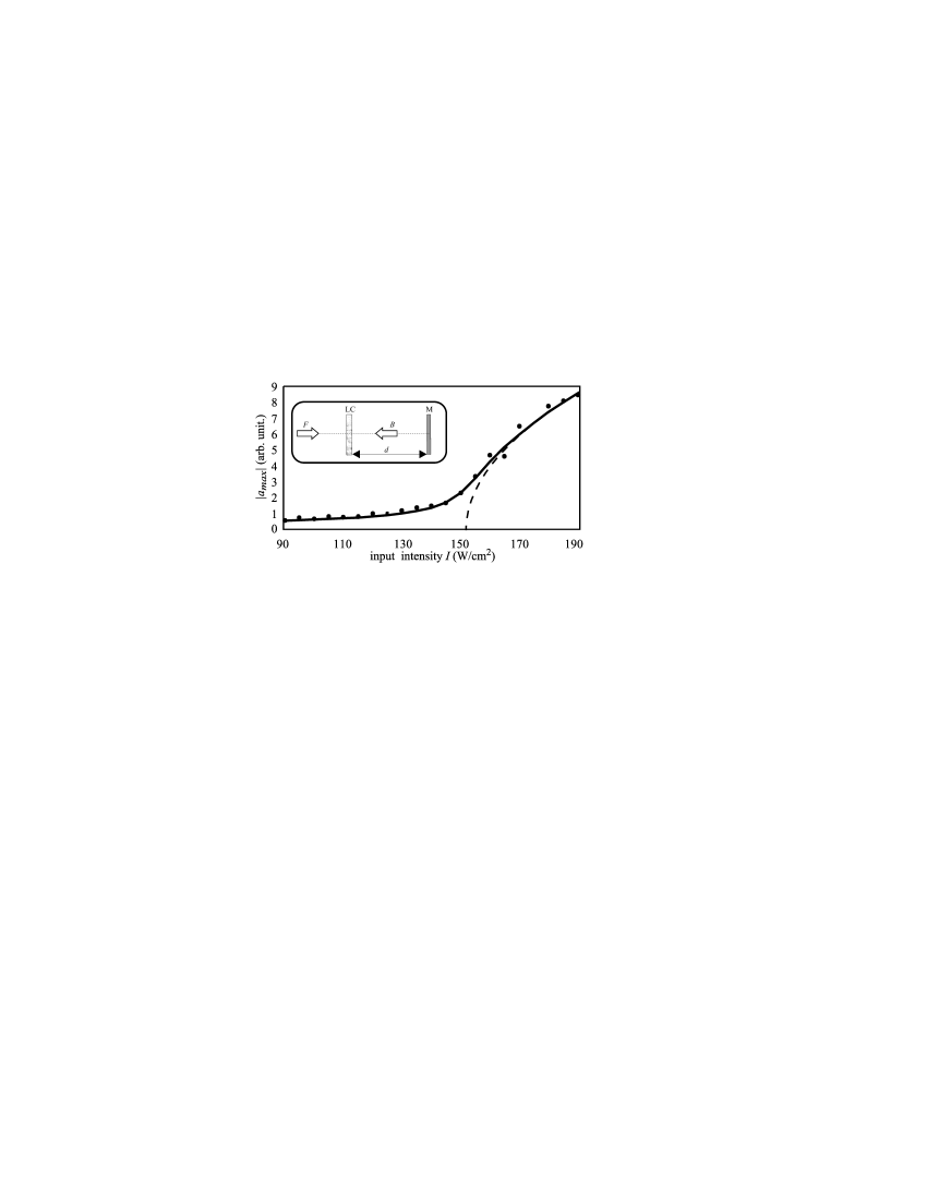
Figure 5: Experimental bifurcation diagram for the optical feedback system. The dots are the experimental measured values of $|a_{max}|$ and the continuous curve its fitted analytical value (Eq. 6). The dashed line is the corresponding deterministic bifurcation deduced from the fit. The inset figure is a schematic sketch of the experimental set-up. LC liquid crystal layer; M feedback mirror; $F$ input optical field; $B$ backward optical field; $d$ feedback length.

Eq. (7) is similar to Eq. (1) and the spatial variations of the pumping beam around its maximum are slow (less than 5% for a domain width $L$ including 4 to 5 rolls) due to the high transverse aspect ratio ($2wk_{c}/2\pi\geq 30$), so that the previous analysis can be applied to describe the supercritical bifurcation of our experimental noisy system. On Fig. 5 we have plotted the experimental recordings of the amplitude expectation value $|a_{max}|$ together with its analytical expression [Eq. (6)] for a transverse domain width $L$ including 4 to 5 rolls around the center of the Gaussian pumping beam. We can see that the analytical expression fits very well the experimental values. It provides us with the deterministic threshold and noise level, $I_{th}=\left|F_{th}\right|^{2}=152\>W.cm^{-2}$ and $\eta=0.01$ respectively. $\eta$ is in very good agreement with previous determinations Gonzague ; Gonzague2 . So, the universal amplitude expression of Eq. (6) is valid and relevant to describe the supercritical spatial bifurcation shape of our noisy system even and more generally to describe the supercritical bifurcations of 1D systems in presence of noise .

In conclusion, we have given an universal amplitude equation for 1D systems in presence of noise. From this equation, we have derived an expression for the amplitude expectation value that fully describes the noisy supercritical bifurcation. The agreement with experiments carried out for an 1D pattern forming system is excellent. This amplitude equation can be applied to any second order transition of noisy temporal systems.

We thank Rene Rojas for useful discussions. The simulation software DimX developed at the laboratory INLN in France has been used for some numerical simulations. We thank the support Anillo grant ACT15 and the ECOS-Sud Committee. The CERLA is supported in part by the “Conseil Régional Nord Pas de Calais” and the ”Fonds Européen de Développement Economique des Régions”.

References

- (1) W. Horsthemke and R. Lefever, Noise-induced transitions: Theory and applications in physics, chemistry and biology, (Springer, Berlin, 1984).
- (2) L. Gammaitoni, P. Hänggi, P. Jung and F. Marchesoni, Rev. Mod. Phys. 70, 223 (1998).
- (3) J. Garcia-Ojalvo and J. M. Sancho, Noise in spatially extended systems, (Springer-Verlag, New-York, 1999).
- (4) G. Agez, P. Glorieux, M. Taki, and E. Louvergneaux, Phys. Rev. A 74, 043814 (2006).
- (5) M. G. Zimmermann, R. Toral, O. Piro, and M. San Miguel, Phys. Rev. Lett. 85, 3612 (2000).
- (6) L.Q. Zhou, X. Jia and Q. Ouyang, Phys. Rev. Lett. 88, 138301 (2002).
- (7) R. Müller, K. Lippert, A. Kühnel and U. Behn, Phys. Rev. E 56, 2658 (1997).
- (8) M.G. Clerc, C. Falcon, E. Tirapegui, Phys. Rev. Lett. 94, 148302 (2005); Phys. Rev. E 74, 011303 (2006).
- (9) M. C. Cross and P. C. Hohenberg, Rev. Mod. Phys. 65, 850 (1993), and references therein.
- (10) G. Agez, C. Szwaj, E. Louvergneaux, and P. Glorieux, Phys. Rev. A. 66, 063805 (2002).
- (11) W. Schöpf and W. Zimmermann, Phys. Rev. E 47, 1739 (1993).
- (12) N.G. Van Kampen, Stochastic process in physics and chemistry (North-Holland, Amsterdam 1992).
- (13) M.N. Ouarzazi, P.A. Bois, and M. Taki, Phys. Rev. A 53, 4408 (1996).
- (14) P.C. Hohenberg, and J.B. Swift, Phys. Rev. A. 46, 4773 (1992).
- (15) R. Lefever, and J. W. Turner, Phys. Rev. Lett. 56, 1631 (1986).
- (16) S. A. Akhmanov, M. A. Vorontsov, and V. Yu. Ivanov, JETP Lett. 47, 707 (1988); S. A. Akhmanov, M. A. Vorontsov, V. Yu. Ivanov, A. V. Larichev, and N. I. Zheleznykh, J. Opt. Soc. Am. B 9, 78 (1992).
- (17) W.J. Firth, J. Mod. Opt. 37, 151 (1990). G. D’Alessandro and W.J. Firth, Phys. Rev. Lett. 66, 2597 (1991).
- (18) C. Szwaj, G. Agez, P. Glorieux, and E. Louvergneaux, submitted to Phys. Rev. A.