Solitary waves in plasmonic Bragg gratings

Abstract

Light propagation in a Bragg periodic structure containing thin films with metallic nanoparticles is studied. Plasmonic resonance frequency, Bragg frequency, and light carrier frequency are assumed to be close. Exact solutions describing solitary gap-waves are found, and a light arrest phenomenon due to nonlinearity of plasmonic oscillations is studied.

I Introduction

The field of photonic crystals, driven by its importance for applications in various areas of photonics, has attracted considerable attention during last the ten years 1 -10 . The one-dimensional resonant Bragg grating 1 -5 or resonantly absorbing Bragg reflector  6 -8 has been of particular interest. An idealized model of a resonant Bragg grating often considers a linear homogeneous dielectric host medium containing an array of thin films with resonant atoms or molecules. The thickness of each film is much less than the wavelength of the electromagnetic wave propagating through such a structure. The dynamics of ultrashort light pulses in the gratings containing films embedded with two-level atoms of the grating has been studied in 1 -8 . The transition frequencies of atoms are assumed to be near the Bragg frequency. Light interaction with such gratings was described by equations of reduced Maxwell-Bloch type. This work demonstrated self-induced transparency in these gratings and the existence of the solitary waves in such structures  1 ; 4 ; 6 . It was also shown 8 that bright as well as dark solitons can exist in the spectral gap.

Progress in nanofabrication of novel optical materials has allowed the design of metal-dielectric nanocomposite materials, which have the ability to sustain nonlinear plasmonic oscillations. An example of such a material is a dielectric with embedded metallic nanoparticles R97 -HRF86 . In this paper we consider ultrashort pulse interaction with Bragg structures containing thin films with metallic nanoparticles. The Bragg resonance frequency and carrier wave frequency in our considerations are assumed to be close to the plasmonic resonance frequency of the nanoparticles. Losses in realistic plasmonic oscillations are of considerable importance. Here we consider an idealized case, wherein pulse duration is much shorter than the characteristic time of losses, so that the effects of losses can be neglected. In the limit of the slowly-varying envelope approximation we derive governing equations for two counter-propagating electromagnetic waves interacting with plasmonic oscillation-induced medium polarization. This system of equations represents the two-wave Maxwell-Duffing type model. We find exact solitary wave solutions of this system and, via computer simulations, analyze stability of these solutions.

II Basic Equations

We consider a grating consisting of an array of thin films which are embedded in a linear dielectric medium. In our derivation of the governing equations we follow 1 -8 , wherein Bragg resonance arises if the distance between successive films is $a=\left(\lambda/2\right)m$, $m=1,2,3,\ldots$.

It was shown in Ma06 ; Ma06_1 that counter-propagating electric field waves $\mathcal{A}$ and $\mathcal{B}$ in the slowly-varying envelope approximation satisfy the following system of equations:

$$i\left(\frac{\partial}{\partial x}+\frac{1}{v_{g}}\frac{\partial}{\partial t}\right)\mathcal{A}-\frac{q_{2}}{2}\frac{\partial^{2}}{\partial t^{2}}\mathcal{A}+\Delta q_{0}\mathcal{A} = -\frac{2\pi\omega_{0}}{c\sqrt{\varepsilon}}\langle\mathcal{P}\rangle,$$ (1)

$$i\left(\frac{\partial}{\partial x}-\frac{1}{v_{g}}\frac{\partial}{\partial t}\right)\mathcal{B}+\frac{q_{2}}{2}\frac{\partial^{2}}{\partial t^{2}}\mathcal{B}-\Delta q_{0}\mathcal{B} = +\frac{2\pi\omega_{0}}{c\sqrt{\varepsilon}}\langle\mathcal{P}\rangle,$$ (2)

where $\Delta q_{0}=q_{0}-2\pi/a$ is the mismatch between the carrier wavenumber and the Bragg resonant wavenumber. The description of the evolution of material polarization in the slowly-varying amplitude approximation requires modeling of the thin films’ response to an external light field. The dielectric properties can be attributed to plasmonic oscillations, which are modeled by Lorentz oscillators. The simplest generalizations of this model include anharmonicity of plasmonic oscillations R16 ; LGMS . In this paper we consider an array of thin films containing metallic nanoparticles which have cubic nonlinear response to external fields R97 ; DBNS04 ; R16 .

The macroscopic polarization $P$ is governed by the equation

$$\frac{\partial^{2}P}{\partial t^{2}}+\omega_{d}^{2}P+\Gamma_{a}\frac{\partial P}{\partial t}+\kappa P^{3}=\frac{\omega_{p}^{2}}{4\pi}E,$$

where $\omega_{p}$ is plasma frequency and $\omega_{d}$ is the transition frequency between energy levels resulting from the dimensional quantization. Losses of the plasmonic oscillations are taken into account by the parameter $\Gamma_{a}$. It is assumed that the duration of the electromagnetic pulse is small enough that dissipation effects can be neglected.

Starting from the slowly-varying envelope approximation, standard manipulation leads to

$$i\frac{\partial\mathcal{P}}{\partial t}+(\omega_{d}-\omega_{0})\mathcal{P}+\frac{3\kappa}{2\omega_{0}}|\mathcal{P}|^{2}\mathcal{P}=-\frac{\omega_{p}^{2}}{8\pi\omega_{0}}\mathcal{E}_{int}(x,t).$$ (3)

Terms varying rapidly in time, which are proportional to $\exp(\pm 3i\omega_{0}t)$, are neglected. In this equation $\mathcal{E}_{int}$ is the electric field interacting with metallic nanoparticles. In the problem under consideration we have $\mathcal{E}_{int}=\mathcal{A}+\mathcal{B}$ .

Due to the limitations of nanofabrication, the sizes and shapes of nanoparticles are not uniform. In practice, deviation from a perfectly spherical shape has a much larger impact on a nanoparticle’s resonance frequency than does variation in diameter. This shape variation causes a broadening of the resonance line. The broadened spectrum is characterized by a probability density function $g(\Delta\omega)$ of deviations $\Delta\omega$ from some mean value $\omega_{res}$. When computing the total polarization, all resonance frequencies must be taken into account.

The contributions of the various resonance frequencies are weighted according to the probability density function $g(\Delta\omega)$; the weighted average is denoted by $\langle\mathcal{P}\rangle$ in equations (1),(2). In what follows, $n(\omega_{0})$ denotes the refractive index of the medium containing the array of thin films, and $n_{np}$ is the effective density of the resonant nanoparticles in films. The effective density is equal to $n_{np}=N_{np}(\ell_{f}/a)$, where $N_{np}$ is the bulk density of nanoparticles, $\ell_{f}$ is the width of a film, and $a$ is the lattice spacing.

We study a medium-light interaction in which resonance is the dominant phenomenon. As such, the length of the sample is smaller than the characteristic dispersion length. In this case the temporal second derivative terms in equations (1,2) can be omitted. The resulting equations are the two-wave Maxwell-Duffing equations. They can be rewritten in dimensionless form using the following rescaling:

$$e_{1}=\mathcal{A}/A_{0},\;e_{2}=\mathcal{B}/A_{0},\;p=(4\pi\omega_{0}/[\sqrt{\varepsilon}\omega_{p}A_{0}])\mathcal{P},\;\zeta=(\omega_{p}/2c)x,\;\tau=t/t_{0}.$$

Here $t_{0}=2\sqrt{\varepsilon}/\omega_{p}$, while $A_{0}$ is a characteristic amplitude of counter-propagating fields. In dimensionless form, the two-wave Maxwell-Duffing equations read

$$i\left(\frac{\partial}{\partial\zeta}+\frac{\partial}{\partial\tau}\right)e_{1}+\delta e_{1} = -\langle p\rangle,$$

$$i\left(\frac{\partial}{\partial\zeta}-\frac{\partial}{\partial\tau}\right)e_{2}-\delta e_{2} = +\langle p\rangle,$$ (4)

$$i\frac{\partial p}{\partial\tau}+\Delta p+\mu|p|^{2}p = -(e_{1}+e_{2}),$$

where $\mu=(3\kappa\sqrt{\varepsilon}/\omega_{0}\omega_{p})(\sqrt{\varepsilon}\omega_{p}/4\pi\omega_{0})^{2}A_{0}^{2}$ is a dimensionless coefficient of anharmonicity, $\delta=2\Delta q_{0}(c/\omega_{p})$ is the dimensionless mismatch coefficient, $\Delta=2\sqrt{\varepsilon}(\omega_{d}-\omega_{0})/\omega_{p}$ is the dimensionless detuning of a nanoparticle’s resonance frequency from the field’s carrier frequency.

In a coordinate system rotating with angular frequency $\delta$,

$$e_{1}=f_{1}e^{i\delta\tau},\;\indent e_{2}=f_{2}e^{i\delta\tau},\;\indent p=qe^{i\delta\tau},$$

equations (4) become

$$i\left(\frac{\partial}{\partial\zeta}+\frac{\partial}{\partial\tau}\right)f_{1} = -\langle q\rangle,$$

$$i\left(\frac{\partial}{\partial\zeta}-\frac{\partial}{\partial\tau}\right)f_{2} = +\langle q\rangle,$$ (5)

$$i\frac{\partial q}{\partial\tau}+(\Delta-\delta)q+\mu|q|^{2}q = -(f_{1}+f_{2}).$$

Further simplification of the system (5) can be achieved by introducing new variables

$$f_{s}=-(f_{1}+f_{2}),\indent f_{a}=f_{1}-f_{2},$$

which allow decoupling of one equation from the system of three equations. In these new variables the polarization $q$ is coupled with only one field variable. Simple transformations give

$$\frac{\partial^{2}f_{a}}{\partial\zeta^{2}}-\frac{\partial^{2}f_{a}}{\partial\tau^{2}} = 2i\frac{\partial}{\partial\zeta}\langle q\rangle,$$ (6)

$$\frac{\partial^{2}f_{s}}{\partial\zeta^{2}}-\frac{\partial^{2}f_{s}}{\partial\tau^{2}} = 2i\frac{\partial}{\partial\tau}\langle q\rangle,$$ (7)

$$i\frac{\partial q}{\partial\tau}+(\Delta-\delta)q+\mu|q|^{2}q = f_{s}.$$ (8)

As one can see, we have a coupled system of equations for $f_{s}$ and $q$.

III Solitary Wave Solutions

We consider localized solitary wave solutions of (6)-(8) in the limit of narrow spectral line $\Delta\omega_{g}/\Delta\omega_{s}\ll 1$, where $\Delta\omega_{s}$ and $\Delta\omega_{g}$ are spectral widths of a signal and spectral line $g(\Delta\omega)$. In this case the spectral line can be represented as a Dirac $\delta$-function: $g(\Delta\omega)=\delta(\Delta\omega)$. Equations (7), (8) can then be re-written as follows:

$$\frac{\partial^{2}f_{s}}{\partial\zeta^{2}}-\frac{\partial^{2}f_{s}}{\partial\tau^{2}} = 2i\frac{\partial q}{\partial\tau}$$ (9)

$$i\frac{\partial q}{\partial\tau}+(\Delta-\delta)q+\mu|q|^{2}q = f_{s}$$ (10)

Scaling analysis of this system shows that solitary wave solutions can be represented as

$$f_{s} = f_{0}F_{\Omega}\left(\eta\right)=\frac{1}{\sqrt{\mu}}\left(\frac{2v^{2}}{1-v^{2}}\right)^{3/4}F_{\Omega}\left(\eta\right),$$

$$q = q_{0}Q_{\Omega}\left(\eta\right)=\frac{1}{\sqrt{\mu}}\left(\frac{2v^{2}}{1-v^{2}}\right)^{1/4}Q_{\Omega}\left(\eta\right),$$ (11)

$$\eta = (\zeta-v\tau)\sqrt{\frac{2}{1-v^{2}}}.$$

Here $v$ is velocity of the solitary wave, $\eta$ is a scale-invariant parameter in a coordinate system moving with the solitary wave, and functions $F_{\Omega}$, $Q_{\Omega}$ satisfy the following system of equations:

$$F_{\Omega}^{\prime\prime} = -iQ_{\Omega}^{\prime},$$

$$-iQ_{\Omega}^{\prime}+\Omega Q_{\Omega}+|Q_{\Omega}|^{2}Q_{\Omega} = F_{\Omega}.$$ (12)

The only dimensionless parameter which remains in the system is

$$\Omega=(\Delta-\delta)\sqrt{\frac{1-v^{2}}{2v^{2}}},$$ (13)

which characterizes the deviation of carrier frequency from the plasmonic frequency $\omega_{p}$ and the Bragg resonance frequency $\omega_{Br}$.

The system of ordinary differential equations (12) has integral of motion for pulse-like solutions decaying as $|\eta|\rightarrow\infty$

$$|Q_{\Omega}|^{2}-|F_{\Omega}|^{2}=0.$$

This allows the following parametrization of solutions:

$$F_{\Omega}(\eta)=R(\eta)e^{i\phi(\eta)},\indent Q_{\Omega}(\eta)=R(\eta)e^{i\psi(\eta)},$$

where $R$, $\phi$, and $\psi$ are real-valued functions satisfying

$$R^{\prime} = -R\sin(\phi-\psi),$$

$$\phi^{\prime} = -\cos(\phi-\psi),$$ (14)

$$\psi^{\prime}+\Omega+R^{2} = \cos(\phi-\psi).$$

If we set $\Phi=\phi-\psi$, then we have

$$\Phi^{\prime}-\Omega-R^{2} = -2\cos\Phi,$$

$$R^{\prime} = -R\sin\Phi.$$ (15)

Taking into account equations (15) we have the conservation law

$$\cos\Phi=\frac{R^{2}}{4}+\frac{\Omega}{2}.$$ (16)

Substituting (16) into the second equation of (15) and subsequent integration gives the following expression for $R$:

$$R^{2}=\frac{2\beta^{2}}{\Omega+2\cosh\left\{\beta(\eta-\eta_{0})\right\}},$$ (17)

where $\beta=\sqrt{4-\Omega^{2}}$. The right-hand side is positive real-valued for all $\eta$ if $-2<\Omega<2$. Using the conservation law (16) we obtain an expression for $\Phi$:

$$\Phi=2\arctan\left(\frac{2-\Omega}{\beta}\tanh\left\{\frac{1}{2}\beta(\eta-\eta_{0})\right\}\right).$$ (18)

Now we integrate $\phi^{\prime}=-\cos\Phi$ and find

$$\phi=-\frac{\Omega}{2}(\eta-\eta_{0})-\arctan\left(\frac{2-\Omega}{\beta}\tanh\left\{\frac{\beta}{2}(\eta-\eta_{0})\right\}\right).$$

Finally, we determine $\psi$:

$$\psi = \phi-\Phi$$

$$= -\frac{\Omega}{2}(\eta-\eta_{0})-3\arctan\left(\frac{2-\Omega}{\beta}\tanh\left\{\frac{\beta}{2}(\eta-\eta_{0})\right\}\right).$$

This pulse exists only if value of the parameter $\Omega$ is inside the interval $-2<\Omega<2$. The maximal value of the amplitude of this solitary solution is

$$A=\sqrt{2(2-\Omega)}.$$

The phases $\phi$ and $\psi$ are nonlinear. Their behavior is asymptotically linear as $\eta\rightarrow\pm\infty$. If $\Omega=0$, then the limiting values of the phases satisfy

$$|\phi(\infty)-\phi(-\infty)| = \pi/2,$$

$$|\psi(\infty)-\psi(-\infty)| = 3\pi/2.$$

The total energy of the solitary wave is distributed among the counter-propagating fields and the medium polarization. Here we study energy partition among these components. Using equations (6), (7) and conditions as $|\eta|\rightarrow\infty$, one can show that

$$f_{a}(\eta)=-\frac{1}{v}f_{s}(\eta)=-\frac{f_{0}}{v}F_{\Omega}(\eta).$$ (19)

We are interested in the energies of the dimensionless fields $f_{1}$, $f_{2}$, and of the polarization $q$.

$$f_{1} = \frac{1}{2}(f_{a}-f_{s})=-\frac{f_{0}}{2}\left(\frac{1}{v}+1\right)F_{\Omega}$$

$$f_{2} = -\frac{1}{2}(f_{s}+f_{a})=\frac{f_{0}}{2}\left(\frac{1}{v}-1\right)F_{\Omega}$$

$$q = q_{0}Q$$

Finally, for electric fields $e_{1},e_{2}$ and for polarization $p$ we have

$$e_{1} = -\frac{1}{2\sqrt{\mu}}\left(\frac{2v^{2}}{1-v^{2}}\right)^{3/4}\left(\frac{1}{v}+1\right)\frac{\sqrt{2}~{}\beta}{\sqrt{\Omega+2\cosh\left\{\beta(\eta-\eta_{0})\right\}}}~{}e^{i\alpha_{e}},$$ (20)

$$e_{2} = \frac{1}{2\sqrt{\mu}}\left(\frac{2v^{2}}{1-v^{2}}\right)^{3/4}\left(\frac{1}{v}-1\right)\frac{\sqrt{2}~{}\beta}{\sqrt{\Omega+2\cosh\left\{\beta(\eta-\eta_{0})\right\}}}~{}e^{i\alpha_{e}};$$ (21)

$$p = \frac{1}{\sqrt{\mu}}\left(\frac{2v^{2}}{1-v^{2}}\right)^{1/4}\frac{\sqrt{2}~{}\beta}{\sqrt{\Omega+2\cosh\left\{\beta(\eta-\eta_{0})\right\}}}~{}e^{i\alpha_{p}},$$

$$\alpha_{e} = \delta\tau-\frac{\Omega}{2}(\eta-\eta_{0})-\arctan\left(\frac{2-\Omega}{\beta}\tanh\left\{\frac{\beta}{2}(\eta-\eta_{0})\right\}\right)$$

$$\alpha_{p} = \delta\tau-\frac{\Omega}{2}(\eta-\eta_{0})-3\arctan\left(\frac{2-\Omega}{\beta}\tanh\left\{\frac{\beta}{2}(\eta-\eta_{0})\right\}\right).$$ (22)

The energy of a solitary wave is

$$E_{R}=\int\limits_{-\infty}^{+\infty}|F_{\Omega}(\eta)|^{2}d\eta=8\arctan\sqrt{\frac{2-\Omega}{2+\Omega}}.$$ (23)

Finally we have the energies of electric fields and polarization

$$E_{e_{1}} = \frac{f_{0}^{2}}{4}\left(\frac{1}{v}+1\right)^{2}E_{R},$$

$$E_{e_{2}} = \frac{f_{0}^{2}}{4}\left(\frac{1}{v}-1\right)^{2}E_{R},$$ (24)

$$E_{p} = q_{0}^{2}E_{R}.$$

Ratios of energies in different fields as well as polarization have the following form

$$\frac{E_{e_{1}}}{E_{e_{2}}} = \left(\frac{1+v}{1-v}\right)^{2},$$ (25)

$$\frac{E_{e_{1}}}{E_{p}} = \frac{1}{2}\frac{(1+v)}{(1-v)},$$ (26)

$$\frac{E_{e_{2}}}{E_{p}} = \frac{1}{2}\frac{(1-v)}{(1+v)}.$$ (27)

Therefore, energy partitioning is determined solely by the parameter $v$, which is a dimensionless combination of main system parameters.

IV Numerical simulation

The shape and phase of the incident optical pulse are controllable in a real experimental situation. To model pulse dynamics in the Bragg grating it is natural to consider asymptotic mixed initial-boundary value problem for equations (4). We define initial conditions as

$$p(\zeta,\tau)\rightarrow 0,~{}~{}~{}e_{1}(\zeta,\tau)\rightarrow 0,~{}~{}~{}e_{2}(\zeta,\tau)\rightarrow 0,~{}~{}~{}\tau\rightarrow-\infty,$$ (28)

with no incident field at the right edge of the sample, and with incident field at the left edge defined as follows:

$$e_{1} (-10,\tau)=w\exp(i\theta),$$ (29)

$$w =4.0\exp\left[-\frac{1}{2}\left(\frac{\tau-3.0}{1.5}\right)^{2}\right],\;\;\theta=\arctan\left(\tanh\left[1.5\left(\tau-3.0\right)\right]\right).$$

In our case the spatial simulation domain was chosen as $[-10,40]$. Parameters $\Delta-\delta$ and $\mu$ were given values

$$\Delta=0,\;\;\delta=1,\;\;\mu=1.$$ (30)

As one can see, we gave the initial pulse the same configuration of phase in a topological sense as would be found in a solitary wave solution. This point is important, because otherwise the phase difference cannot relax to the symmetry of the stationary wave which is revealed in (18). As a result, in numerical simulations it is difficult to achieve solitary wave type dynamics of the pulse without the proper phase configuration of the incident pulse.

The second field boundary condition was set to be

$$e_{2}(40,\tau)=0.$$ (31)

In the first experiment we injected a pulse, which is relatively close to the solitary wave solution. The results are shown in Figs. 1-3, which clearly represent two stages of the pulse evolution.

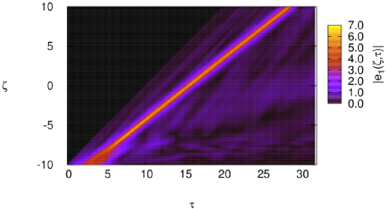
Figure 1: Propagation of pulse. The first experiment. Mapping of the $|e_{1}(\zeta,\tau)|$ surface.

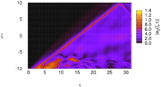
Figure 2: Propagation of pulse. The first experiment. Mapping of the $|e_{2}(\zeta,\tau)|$ surface.

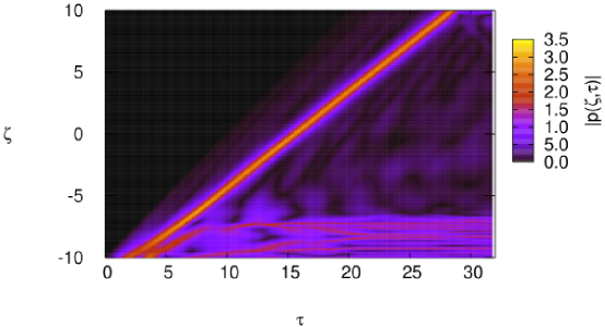
Figure 3: Propagation of pulse. The first experiment. Mapping of the $|p(\zeta,\tau)|$ surface.

In the first stage ($t\leq 7$) of evolution we observed fast excess energy damping in radiation of quasi-linear waves in both directions and relaxation to a solution roughly similar to the stationary solution. Then we observed a stage of pulse shape refinement ($7<t<30$) with consequent propagation of the solution very close to (17). The lower part of the figure 3 shows the creation of multiple spatially frozen “hot spots” of the medium polarization. In these hot spots the energy of oscillations is arrested in the grating. This “stopping light” phenomenon is due to self-modulation of the medium polarization caused by nonlinear effects which we shall discuss in more detail elsewhere.

During the second experiment we used a pulse of lower amplitude:

$$e_{1}(-10,\tau) = w\exp(i\theta),$$

$$w = 3.3\exp\left[-\frac{1}{2}\left(\frac{\tau-3.0}{1.5}\right)^{2}\right],$$

$$\theta = \arctan\left(\tanh\left[1.5\left(\tau-3.0\right)\right]\right).$$ (32)

Results are represented in Figs. 4-6.

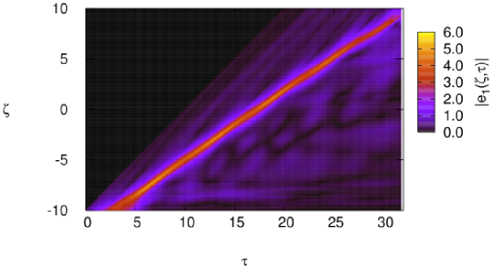
Figure 4: Propagation of pulse. The second experiment. Mapping of the $|e_{1}(\zeta,\tau)|$ surface.

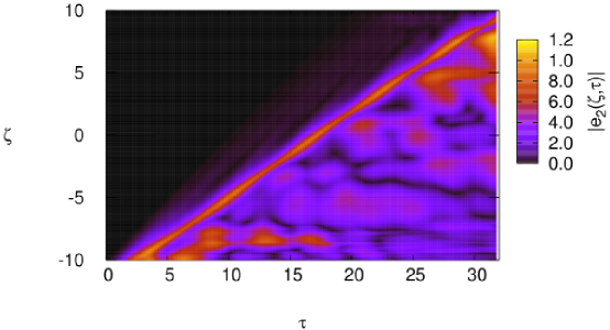
Figure 5: Propagation of pulse. The second experiment. Mapping of the $|e_{2}(\zeta,\tau)|$ surface.

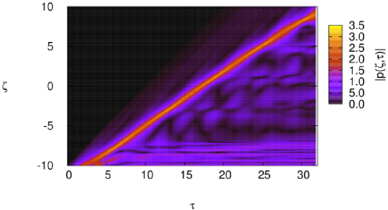
Figure 6: Propagation of pulse. The second experiment. Mapping of the $|p(\zeta,\tau)|$ surface.

Deviation of the incident pulse from exact solitary wave solution was stronger in the second numerical experiment. In this case, computer simulations clearly demonstrate oscillatory behavior of the pulse dynamics. Study of the origin of such oscillations will also be presented in a separate publication. In both cases we observed a phenomenon similar to self-induced transparency in nanocomposite materials described in R16 . These solitary wave solutions represent the phenomenon of nonlinear light trapping when the wave of medium polarization is bound by two optical light fields propagating in the same direction. In the linear limit these two optical fields are propagating in opposite directions.

V Conclusion

We studied, both analytically and numerically, solitary waves describing coupled medium polarization and light propagation in Bragg gratings with thin films containing metallic nanoparticles. We observed self-induced transparency-like phenomena and formation of polarization “hot spots”. The formation of solitary wave solutions occurs when energy of an incident pulse exceeds some threshold value. The lower boundary value of this threshold can be evaluated as sum of energies (24) of electric and plasmonic components of coupled wave.

Stability of nonlinear solitary waves is an important problem which can be addressed by study of collision properties and analysis of localized modes of such waves. This problem is the subject of our future investigations.

References

• (1) B. I. Mantsyzov and R. N. Kuzmin, Sov. Phys. JETP, 64, 37-44 (1986).
• (2) B. I. Mantsyzov and D. O. Gamzaev, Optics and spectroscopy, 63, 1, 200-202 (1987).
• (3) T. I. Lakoba and B. I. Mantsyzov, Bull. Russian Acad. Sci. Phys., 56, 8, 1205-1208 (1992).
• (4) B. I. Mantsyzov, Phys.Rev. A, 51, 6, 4939-4943 (1995).
• (5) B. I. Mantsyzov and E. A. Silnikov, J. Opt. Soc. Amer. B, 19, 2203-2207 (2002).
• (6) B. I. Mantsyzov, JETP letters, 82, 5, 253-258 (2005).
• (7) A. Kozhekin and G. Kurizki, Phys. Rev. Lett., 74, 25, 5020-5023 (1995).
• (8) A. Kozhekin, G. Kurizki, and B. Malomed, Phys. Rev. Lett., 81, 17, 3647-3650 (1998).
• (9) T. Opatrny, B. A. Malomed, and G. Kurizki, Phys. Rev. E,  60, 5, 6137-6149 (1999).
• (10) G. Kurizki, A. E. Kozhekin, T. Opatrny, and B. A. Malomed, Progr. Optics, 42, 93-146 (E. Wolf, editor: North Holland, Amsterdam, 2001).
• (11) J. Cheng and J. Zhou, Phys. Rev. E, 66, 036606 (2002)
• (12) V. I. Rupasov, V. I. Yudson, Quantum electronics (in Russian), 9, 2179 (1982).
• (13) S. G. Rautian, JETP, 85, 451–461 (1997).
• (14) V. P. Drachev, A. K. Buin, H. Nakotte, and V. M. Shalaev, Nano Lett., 4, 1535–1539 (2004).
• (15) F. Hache, D. Ricard, and C. Flytzanis, J. Opt. Soc. Am. B, 3, 1647–1655 (1986).
• (16) N. M. Lichinitser, I. R. Gabitov, A. I. Maimistov, and V. M. Shalaev, Optics Lett., 32, 2, 151-153 (2007).
arXiv:physics/0607177
• (17) A. I. Maimistov, arXiv: nlin.PS/0607012
• (18) I. R. Gabitov, A. O. Korotkevich, A. I. Maimistov, and J. B. McMahon, arXiv: nlin.PS/0702035
• (19) I. R. Gabitov, R. A. Indik, N. M. Litchinitser, A. I. Maimistov, V. M. Shalaev, J. E. Soneson, J. Opt. Soc. Am. B, 23, 535-542 (2006).