Noise-induced Turbulence in Nonlocally Coupled Oscillators

Abstract

We demonstrate that nonlocally coupled limit-cycle oscillators subject to spatiotemporally white Gaussian noise can exhibit a noise-induced transition to turbulent states. After illustrating noise-induced turbulent states with numerical simulations using two representative models of limit-cycle oscillators, we develop a theory that clarifies the effective dynamical instabilities leading to the turbulent behavior using a hierarchy of dynamical reduction methods. We determine the parameter region where the system can exhibit noise-induced turbulent states, which is successfully confirmed by extensive numerical simulations at each level of the reduction.

I Introduction

When a dynamical system is driven by external noises, its effective dynamics generally changes ref:horsthemke84 ; ref:ojalvo99 ; ref:anishchenko01 ; ref:matsumoto83 ; ref:shibata99 . We usually expect that the system tends to be more random and statistically uniform, because the noise destroys the spatiotemporal structures of the system. For example, Matsumoto and Tsuda ref:matsumoto83 found that external noise can destabilize chaos and produces ordered behavior in the Belousov-Zhabotinsky map, and called this phenomenon “noise-induced order”. Shibata, Chawanya, and Kaneko ref:shibata99 studied the effect of microscopic external noise on the collective motion of a globally coupled map in fully desynchronized states. They demonstrated that the collective motion is successively simplified with the increase of external noise intensity, while without the external noise a macroscopic variable shows high-dimensional chaos distinguishable from random motions.

In this paper, we give a counter-example to this intuition. Specifically, we demonstrate that nonlocally coupled limit-cycle oscillators can undergo a noise-induced transition from uniform states to turbulent states through effective dynamical instabilities, with the induced turbulent fluctuations far larger than the intensity of the driving noise.

Our starting point is a general equation describing nonlocally coupled limit-cycle oscillators subject to spatiotemporally white Gaussian noise. We first present numerical examples using two representative models of limit-cycle oscillators, the FitzHugh-Nagumo model and the Stuart-Landau model, in order to illustrate that weak external noise can actually cause turbulence in such systems. To theoretically investigate this noise-induced turbulent state, we simplify our original equation to a Langevin phase equation by means of the phase reduction method for limit-cycle oscillators, utilizing the fact that the external noise intensity and the coupling strength between the oscillators are sufficiently weak. The resulting equation describes a system of nonlocally coupled noisy phase oscillators. We then derive an equivalent nonlinear Fokker-Planck equation from this Langevin equation by adopting the mean-field theory, which holds exactly for our nonlocally coupled oscillators. Our nonlinear Fokker-Planck equation has a constant solution corresponding to all the oscillators being in a completely desynchronized state. It is linearly stable when the external noise is sufficiently strong, but, as the noise intensity is decreased, undergoes a Hopf bifurcation at a certain noise intensity, giving rise to limit-cycle oscillations of the phase distribution. In the vicinity of this bifurcation point, we can derive a complex Ginzburg-Landau equation from the nonlinear Fokker-Planck equation by applying the center-manifold reduction method, which governs the small-amplitude deviation of the probability density from the constant solution. It is well known that the spatially uniform oscillation of the complex Ginzburg-Landau equation becomes unstable and spatiotemporal chaos develops when the Benjamin-Feir instability condition is satisfied. Therefore, we expect that the Langevin phase equation and the corresponding nonlinear Fokker-Planck equation also exhibit spatiotemporal chaos under suitable conditions. By direct numerical simulations, we will confirm that the amplitude turbulence typical of the complex Ginzburg-Landau equation actually arises. In addition, we also confirm that the phase turbulence arises near the Benjamin-Feir criticality, which is also a hallmark of the complex Ginzburg-Landau equation. We then examine the situation far from the Hopf bifurcation. In our system, another smaller critical noise intensity is expected to exist, above which the turbulence arises from the spatially uniform oscillation via a long-wave phase instability. To confirm this, we derive a Kuramoto-Sivashinsky-type equation by applying the phase reduction method to the spatially uniform oscillating solution of the nonlinear Fokker-Planck equation. Our calculation shows that the phase diffusion coefficient changes its sign from positive to negative as the noise intensity is increased from zero, which implies the destabilization of the spatially uniform oscillating solution. By a systematic numerical calculation of the phase diffusion coefficient, we determine the parameter region where our system exhibits a noise-induced turbulent state. From the mathematical analysis of the hierarchy of reduced equations and extensive numerical simulations of the dynamical equation at each level of the reduction, we will conclude that the appearance of the turbulence can be considered as a noise-induced transition phenomenon.

The organization of this paper is as follows. In Sec. II, we introduce our model and present numerical results for the FitzHugh-Nagumo and Stuart-Landau oscillators. In Sec. III, we derive Langevin and Fokker-Planck equations from the original equation by the phase reduction method. In Sec. IV, we derive a complex Ginzburg-Landau equation by a center-manifold reduction of the Fokker-Planck equation near its Hopf bifurcation point. In Sec. V, we reduce the Fokker-Planck equation to a Kuramoto-Sivashinsky-type equation near the destabilization point of the spatially uniform oscillation, and draw the complete phase diagram of the noise-induced turbulence. Concluding remarks will be given in the final section.

II Noise-induced turbulence in nonlocally coupled limit-cycle oscillators

In this section, we introduce a general model of nonlocally coupled noisy oscillators, and numerically demonstrate that the model can exhibit noise-induced turbulent states using two representative models of limit-cycle oscillators.

II.1 General model

We consider a system of nonlocally coupled limit-cycle oscillators in one-dimensional space subject to spatiotemporal noise. The general form of the model is given by

$$\partial_{t}\mbox{\boldmath$X$}\left(x,t\right)=\mbox{\boldmath$F$}\left(\mbox{\boldmath$X$}\left(x,t\right)\right)+\hat{K}\int_{-\infty}^{\infty}dx^{\prime}\,G\left(x-x^{\prime}\right)\mbox{\boldmath$X$}\left(x^{\prime},t\right)+\sqrt{\sigma}\,\mbox{\boldmath$\eta$}\left(x,t\right).$$ (1)

Here, $\mbox{\boldmath$X$}(x,t)$ represents the state of a local limit-cycle oscillator at location $x$ and time $t$. The first term on the right-hand side describes the dynamics of each oscillator. In the absence of the coupling and the noise, it is simply given by $\dot{\mbox{\boldmath$X$}}=\mbox{\boldmath$F$}(\mbox{\boldmath$X$})$, which is assumed to have a single stable limit-cycle solution. The second term describes the nonlocal coupling among the oscillators, where $\hat{K}$ and $G(x)$ represent respectively the coupling matrix and the nonlocal coupling function. Throughout this paper, we use a simple exponential function

$$G\left(x\right)=\frac{1}{2}\exp\left(-\left|x\right|\right),$$ (2)

which is normalized to unity in the whole space domain. The last term of Eq. (1) represents the external noise applied to each oscillator, whose intensity is controlled by the parameter $\sigma$. $\mbox{\boldmath$\eta$}(x,t)$ is a spatiotemporally white Gaussian noise with zero mean specified by

$$\left\langle\eta_{j}\left(x,t\right)\right\rangle=0,\quad\left\langle\eta_{j}\left(x,t\right)\eta_{j^{\prime}}\left(x^{\prime},t^{\prime}\right)\right\rangle=2\delta_{j,j^{\prime}}\delta\left(x-x^{\prime}\right)\delta\left(t-t^{\prime}\right),$$ (3)

where the subscripts $j$ and $j^{\prime}$ denote the vector components of the noise.

Equation (1) can naturally be derived, for example, in the following situation. Let us consider a set of equations ref:kuramoto06 ; ref:kuramoto95 ; ref:kuramoto98 ; ref:kuramoto00 ; ref:tanaka03 ; ref:shima04

$$\partial_{t}\mbox{\boldmath$X$}\left(x,t\right) =\mbox{\boldmath$F$}\left(\mbox{\boldmath$X$}\left(x,t\right)\right)+\hat{K}\mbox{\boldmath$S$}\left(x,t\right)+\sqrt{\sigma}\,\mbox{\boldmath$\eta$}\left(x,t\right),$$ (4)

$$\tau\partial_{t}\mbox{\boldmath$S$}\left(x,t\right) =-\mbox{\boldmath$S$}\left(x,t\right)+\partial_{x}^{2}\mbox{\boldmath$S$}\left(x,t\right)+\mbox{\boldmath$X$}\left(x,t\right),$$ (5)

which describe a system of mutually interacting oscillatory elements, where the coupling between the elements is mediated by some substance that diffuses and decays much faster than the dynamics of the individual oscillators, e.g. slime molds interacting through signal molecules. By considering the $\tau\to 0$ limit and eliminating the fast dynamics of $S$ adiabatically, we obtain Eq. (1) with the kernel given by Eq. (2) from Eqs. (4)-(5).

II.2 FitzHugh-Nagumo oscillators

As the first example, we consider the case that the local oscillator in Eq. (1) is given by the FitzHugh-Nagumo (FN) oscillator. The model is explicitly given by

$$\partial_{t}X(x,t) =F_{X}(X,Y)+K_{X}S_{X}(x,t)+\sqrt{\sigma}\,\eta_{X}(x,t),$$ (6)

$$\partial_{t}Y(x,t) =F_{Y}(X,Y)+K_{Y}S_{X}(x,t)+\sqrt{\sigma}\,\eta_{Y}(x,t),$$ (7)

where the dynamics of each oscillator is described by

$$F_{X}(X,Y)=\epsilon^{-1}\left(X-X^{3}-Y\right),\quad F_{Y}(X,Y)=aX+b,$$ (8)

and the nonlocal coupling term $S_{X}(x,t)$ is given by

$$S_{X}\left(x,t\right)=\int_{-\infty}^{\infty}dx^{\prime}\,G\left(x-x^{\prime}\right)X\left(x^{\prime},t\right).$$ (9)

We consider the case that the oscillators are coupled only through the variable $X$. We fix the parameters of the oscillators as $\epsilon=0.5$, $a=1.0$, and $b=0.3$, with which the oscillators are well in the self-oscillatory regime.

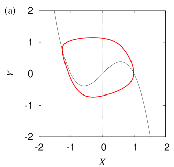
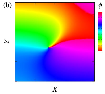
Figure 1: (Color online) FitzHugh-Nagumo oscillator with parameters $\epsilon=0.5$, $a=1.0$, and $b=0.3$. (a): Limit-cycle orbit and nullclines in the $X$-$Y$ plane. (b): Generalized phase $\phi(X,Y)\in[0,2\pi]$, which is globally defined such that $\dot{\phi}=\omega$ holds identically.

Figure 1(a) shows the limit-cycle orbit of an individual FitzHugh-Nagumo oscillator in the $X$-$Y$ plane together with its nullclines, in the absence of the coupling and the noise. Throughout this paper, we use a generalized phase variable to describe the oscillator (see the next section). Figure 1(b) shows the generalized phase variable of the FitzHugh-Nagumo oscillator defined on the $X$-$Y$ plane, which maps the state variable $(X,Y)$ of the oscillator to a single real phase variable $\phi\in[0,2\pi]$.

We performed direct numerical simulations of Eqs. (6)-(9), where the oscillator fields $X(x,t)$ and $Y(x,t)$ are discretized using $N=2^{10}$ oscillators with the spatial grid size of $\Delta x=0.1$. See Appendix C for the details of the numerical methods. The values of the coupling strength $K_{X}$ and $K_{Y}$ are chosen appropriately in such a way that the spatially uniform oscillation is stable and the system is non-turbulent in the absence of noise.

In order to observe the average deterministic dynamics of the system, it is desirable to filter statistical fluctuations due to the noise. We thus introduce a space-time dependent complex order parameter with modulus $R(x,t)$ and phase $\Theta(x,t)$, calculated from the oscillator phase field $\phi(x,t)$ through

$$R\left(x,t\right)\exp\Bigl{(}i\Theta\left(x,t\right)\Bigr{)}=\int_{-\infty}^{\infty}dx^{\prime}\,G\left(x-x^{\prime}\right)\exp\Bigl{(}i\phi\left(x^{\prime},t\right)\Bigr{)}.$$ (10)

This order parameter represents a spatial average of the complex phase factor $\exp(i\phi)$ of the local oscillators over the coupling range.

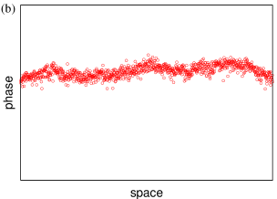
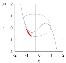
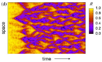
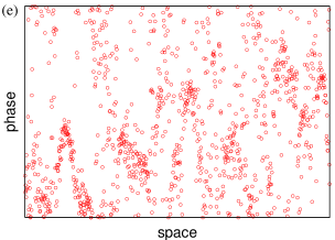
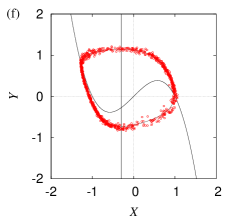
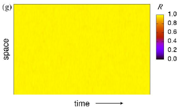
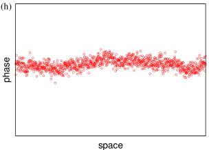
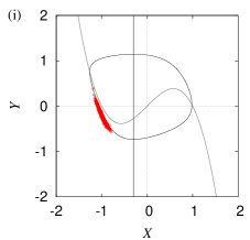
Figure 2: (Color online) Numerical simulations of nonlocally coupled noisy FitzHugh-Nagumo oscillators for three representative cases. (a), (b), and (c): Case FN-I ($K_{X}=0.02$, $K_{Y}=0.08$, and $\sigma=0.0002$); (d), (e), and (f): Case FN-II ($K_{X}=0.02$, $K_{Y}=0.08$, and $\sigma=0.0006$); (g), (h), and (i): Case FN-III ($K_{X}=0.08$, $K_{Y}=0.02$, and $\sigma=0.0006$). Other parameters are fixed as $\epsilon=0.5$, $a=1.0$, and $b=0.3$. The left panels (a), (d), and (g) show spatiotemporal patterns of the order parameter modulus; the middle panels (b), (e), and (h) show instantaneous spatial profile of the local oscillator phase; the right panels (c), (f), and (i) show corresponding phase portraits in the $X$-$Y$ plane. The number of oscillators is $N=2^{10}$ and the separation between neighboring oscillators is $\varDelta x=0.1$.

Results for three representative cases, denoted by FN-I, FN-II, and FN-III, are illustrated in Fig. 2 in rows. The left panels display the spatiotemporal evolution of the modulus $R(x,t)$ of the order parameter, the middle panels display how the phases of the individual oscillators are distributed in space at a given time, and the right panels display the snapshots of the state variables of the oscillators on the $X$-$Y$ plane.

To see what happens when we increase the noise intensity from zero, we first compare the cases FN-I (top row) and FN-II (middle row). The coupling parameters used in FN-I and FN-II are the same, but the noise intensity used in FN-II is three times stronger than that used in FN-I. In the weak noise case, FN-I, the modulus of the order parameter (left panel) is almost uniform in space and also constant in time. The phases of the individual oscillators (middle and right panels) somewhat fluctuate due to the noise, but the amplitude of the fluctuation seems to be much smaller than that we expect for turbulent fluctuations due to a dynamical instability of the system. In the case FN-II, the noise is three times stronger. Now the modulus of the order parameter exhibits quite irregular spatiotemporal behavior, and the amplitude of the phase fluctuations is much larger than that in the case FN-I, covering the whole range from $0$ to $2\pi$. Note also that the amplitude of the phase fluctuations is far larger than the applied noise intensity, which indicates that they are produced by a noise-induced dynamical instability of the system.

Only with these results, it might still be suspected that what looks like turbulence in the case FN-II might actually not be true turbulence, and the large fluctuations of the order parameter might simply be the result of increasing the noise intensity by three times. To clear up this suspicion, we compare the cases FN-II (middle row) and FN-III (bottom row). Now the noise intensities are the same, but the coupling parameters are slightly different. As clearly be seen, the order parameter observed in the case FN-III is almost uniform in space and constant in time at the same noise level as that used in the case FN-II. Therefore, the violent order parameter fluctuations in the case FN-II should not simply be statistical ones due to the noise.

To distinguish the two types of order parameter fluctuations more clearly, we systematically vary the total number $N$ of the oscillators in each case. Since we fix the system length, we are controlling the oscillator number density, or equivalently, the number of oscillators sitting within the coupling range. If the fluctuation of the order parameter is simply of statistical origin coming from the finiteness of $N$, the variance should decrease as $N^{-1}$ due to the central limit theorem. In contrast, if the order parameter fluctuation is due to the dynamical instability of the system, the same quantity should remain constant even if $N$ is varied.

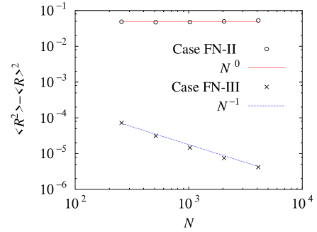
Figure 3: (Color online) Order parameter fluctuation $\langle R^{2}\rangle-\langle R\rangle^{2}$ vs. oscillator number $N$ for the Case FN-II (open circles) and the Case FN-III (crosses). $\langle\cdot\rangle$ represents the space-time average. The solid and dashed lines have slopes 0 and -1, respectively. The system size is fixed as $L=N\varDelta x=102.4$.

The results are shown in Fig. 3, where the variance of each order parameter is plotted as a function of $N$ in double-logarithmic scales for the cases FN-II and FN-III. We see that there is a vast difference in the amplitude of fluctuations, and, as expected, its dependence on $N$ is clearly different between the two cases; the fluctuation amplitude is almost constant in the case FN-II, whereas it decreases in inverse proportion to $N$ in the case FN-III.

Thus, we conclude that the phase fluctuations observed in the case FN-II is not merely finite-sample statistical fluctuations, but they are actually turbulent fluctuations generated by the effective dynamical instability of the system induced by the weak external noise.

II.3 Stuart-Landau oscillators

Our second example is a system of Stuart-Landau (SL) oscillators with nonlocal coupling, which is described by

$$\partial_{t}W(x,t)=\left(1+i\omega_{0}\right)W-\left(1+i\beta\right)\left|W\right|^{2}W+KS_{W}(x,t)+\sqrt{\sigma}\,\eta_{W}(x,t),$$ (11)

and

$$S_{W}\left(x,t\right)=\int_{-\infty}^{\infty}dx^{\prime}\,G\left(x-x^{\prime}\right)W\left(x^{\prime},t\right).$$ (12)

The Stuart-Landau oscillator is the simplest limit-cycle oscillator derived as a normal form of the supercritical Hopf bifurcation ref:kuramoto84 . Each oscillator state is now described by a complex amplitude, $W$. Correspondingly, the coupling term $S_{W}$ and the noise $\eta_{W}$ are also complex variables. We take the parameters $\omega$ and $K$ as $\omega_{0}=\beta+1.0$ and $K=0.05$, and control the remaining parameters $\beta$ and $\sigma$. As in the previous FitzHugh-Nagumo case, the values of the parameter $\beta$ is chosen in such a way that the spatially uniform oscillation is stable and the system is non-turbulent in the absence of noise.

We carried out the numerical analysis of this model completely in parallel with the previous case of the FitzHugh-Nagumo oscillators (see Appendix C for the numerical methods). For the Stuart-Landau oscillator, mapping from the complex amplitude $W$ to the generalized phase $\phi$ can be analytically given as ref:kuramoto84 ; ref:pikovsky01

$$\phi=\arg W-\beta\ln\left|W\right|.$$ (13)

Using this definition, we calculate the order parameter of the system given by Eq. (10).

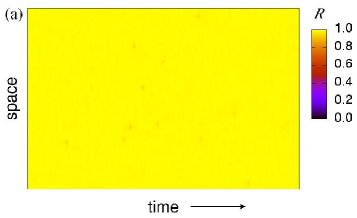
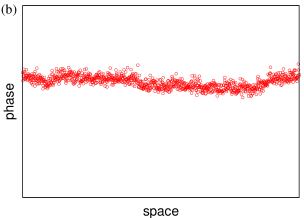
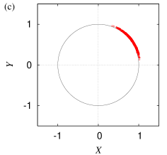
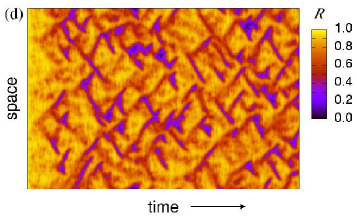
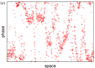
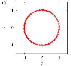
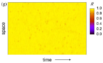
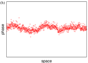
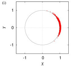
Figure 4: (Color online) Numerical simulations of nonlocally coupled noisy Stuart-Landau oscillators for three representative cases. (a), (b), and (c): Case SL-I ($\beta=2.6$ and $\sigma=0.0001$); (d), (e), and (f): Case SL-II ($\beta=2.6$ and $\sigma=0.0006$); (g), (h), and (i): Case SL-III ($\beta=1.6$ and $\sigma=0.0006$). Other parameters are given by $\omega_{0}=\beta+1.0$ and $K=0.05$. The left panels (a), (d), and (g) show the spatiotemporal patterns of the order parameter modulus; the middle panels (b), (e), and (h) show the instantaneous spatial profile of the local oscillator phase; the right panels (c), (f), and (i) show the corresponding phase portraits in the $X$-$Y$ plane. The number of oscillators is $N=2^{10}$ and the separation between neighboring oscillators is $\varDelta x=0.1$.

Figure 4 summarizes the numerical results, where three representative cases SL-I, SL-II, and SL-III are compared. As previous, the parameter $\beta$ is the same for SL-I and SL-II, but the noise intensity in SL-II is six times larger than that in SL-I. In the case SL-I, the amplitude of the phase fluctuations is quite small, and the modulus $R(x,t)$ of the order parameter is almost spatially uniform and temporally constant. In the case SL-II, the amplitude of the phase fluctuations becomes quite large, and the modulus $R(x,t)$ of the order parameter exhibits complex spatiotemporal dynamics. Thus, the strong turbulent fluctuation arises from the spatially uniform oscillation as the noise intensity is increased. However, when the parameter $\beta$ is slightly changed, SL-III, the noise with the same intensity cannot induce such turbulent fluctuations.

From the same argument as the previous FitzHugh-Nagumo case, we conclude that the strong fluctuation seen in the case SL-II represents a genuine turbulence of the dynamical origin induced by the external noise.

III Reduction to Nonlocally coupled noisy phase oscillators

We have observed that nonlocally coupled limit-cycle oscillators can exhibit noise-induced turbulent states. In the present and the subsequent sections, we will develop a theory that explains consistently the above numerical results. In this section, we present our first step, namely, the derivation of a Langevin phase equation from the original dynamical equation for the nonlocally coupled limit cycles by means of the phase reduction method. The resulting equation describes a system of nonlocally coupled phase oscillators, whose validity is demonstrated numerically for the Stuart-Landau oscillators. We also derive an equivalent nonlinear Fokker-Planck equation through the mean-field theory, which will be the starting point for further analysis.

III.1 Phase reduction

We apply the standard phase reduction method to our system of nonlocally coupled noisy limit-cycle oscillators, which derives an approximate equation consisting of only the phase variable from the original dynamical equations in multiple variables ref:kuramoto84 . The phase reduction is allowed when the individual local oscillators are perturbed only slightly. Thus, the coupling strength and the external noise intensity should be sufficiently small. As shown in the phase portraits in Figs. 2 and 4 (right panels), the oscillators are always in the near vicinity of the unperturbed limit-cycle orbits. Therefore, the parameter values used in the previous numerical analysis satisfy the above condition.

As we already mentioned, we use a specific definition of the phase, determined on the phase space of the limit cycle in such a way that $\dot{\phi}=\omega$ holds identically, where $\omega$ is the natural frequency of the local oscillator. This can always be done by an appropriate nonlinear transformation of the phase space variables of the oscillator ref:winfree80 ; ref:kuramoto84 ; ref:pikovsky01 .

Details of the derivation of a phase equation from Eq. (1) are given in Appendix A. The resulting phase equation takes the form

$$\partial_{t}\phi\left(x,t\right)=\omega+\int^{\infty}_{-\infty}dx^{\prime}\,G\left(x-x^{\prime}\right)\Gamma\bigl{(}\phi(x,t)-\phi(x^{\prime},t)\bigr{)}+\sqrt{D}\,\xi\left(x,t\right),$$ (14)

where $\Gamma(\phi)$ represents the phase coupling function between the oscillators, $D$ the effective noise intensity that inherits the effect of the noise $\mbox{\boldmath$\eta$}(x,t)$ in the original equation, and $\xi(x,t)$ a real scalar spatiotemporally white Gaussian noise satisfying

$$\left\langle\xi\left(x,t\right)\right\rangle=0,\quad\left\langle\xi\left(x,t\right)\xi\left(x^{\prime},t^{\prime}\right)\right\rangle=2\delta\left(x-x^{\prime}\right)\delta\left(t-t^{\prime}\right).$$ (15)

The phase coupling function $\Gamma(\phi)$ can be calculated from the dynamical equations of the coupled limit cycles. The effective noise intensity $D$ can also be calculated once the parameters of the original dynamical equations are given. Note that the above equation describes a system of nonlocally coupled noisy phase oscillators.

III.2 FitzHugh-Nagumo oscillators

We first consider the case of the FitzHugh-Nagumo oscillators. By applying the formula developed in Appendix A, the phase coupling function can be expressed as

$$\Gamma\left(\phi-\phi^{\prime}\right)=\frac{1}{2\pi}\int_{0}^{2\pi}d\lambda\;\Bigl{[}K_{X}Z_{X}\left(\lambda+\phi\right)+K_{Y}Z_{Y}\left(\lambda+\phi\right)\Bigr{]}X_{0}\left(\lambda+\phi^{\prime}\right),$$ (16)

where $X_{0}(\phi)$ is the $X$-component of the unperturbed limit cycle, and $Z_{X}(\phi)$ and $Z_{Y}(\phi)$ are the phase sensitivity functions of the FitzHugh-Nagumo oscillator. Though the limit-cycle solution of the FitzHugh-Nagumo model cannot be obtained analytically, these quantities can be calculated numerically with sufficient precision using standard methods ref:izhikevich07 .

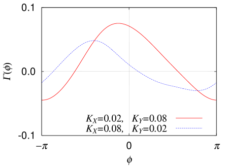
Figure 5: (Color online) Phase coupling functions $\Gamma(\phi)$ of the FitzHugh-Nagumo oscillators. The solid and dashed curves correspond to the Cases FN-I and FN-II ($K_{X}=0.02$ and $K_{Y}=0.08$) and the Case FN-III ($K_{X}=0.08$ and $K_{Y}=0.02$), respectively. The in-phase coupling condition is satisfied in both cases, i.e., $d\Gamma(\phi)/d\phi|_{\phi=0}<0$.

Figure 5 displays the phase coupling function $\Gamma(\phi)$ calculated for the two sets of the coupling constants $K_{X}$ and $K_{Y}$ used in section II. For both parameter conditions, the coupling functions are the in-phase type, as is clear from the property $d\Gamma(\phi)/d\phi|_{\phi=0}<0$ ref:kuramoto84 .

The effective noise intensity $D$ can be expressed by the original noise intensity $\sigma$ and the phase sensitivity functions $Z_{X}$ and $Z_{Y}$ as

$$D=\frac{1}{2\pi}\int_{0}^{2\pi}d\lambda\;\sigma\Bigl{[}Z_{X}^{2}(\lambda)+Z_{Y}^{2}(\lambda)\Bigr{]}.$$ (17)

III.3 Stuart-Landau oscillators

In the case of the Stuart-Landau oscillators, the limit-cycle solution and the phase sensitivity function can be obtained analytically. The natural frequency, the phase coupling function, and the effective noise intensity are given by $\tilde{\omega}=\omega_{0}-\beta$, $\Gamma(\phi-\phi^{\prime})=-K\sqrt{1+\beta^{2}}\sin(\phi-\phi^{\prime}+\alpha)$, and $\tilde{D}=\sigma(1+\beta^{2})$, respectively. Thus, Eq. (14) takes the following explicit form

$$\partial_{t}\phi(x,t)=\tilde{\omega}-K\sqrt{1+\beta^{2}}\int_{-\infty}^{\infty}dx^{\prime}\,G\left(x-x^{\prime}\right)\sin\bigl{(}\phi(x,t)-\phi(x^{\prime},t)+\alpha\bigr{)}+\sqrt{\tilde{D}}\,\xi\left(x,t\right),$$ (18)

where the parameter $\alpha$ is given by

$$\alpha=\arg\left(1+i\beta\right).$$ (19)

By changing the time scale, we can simplify the above equation as

$$\partial_{t}\phi\left(x,t\right)=\omega-\int_{-\infty}^{\infty}dx^{\prime}\,G\left(x-x^{\prime}\right)\sin\bigl{(}\phi(x,t)-\phi(x^{\prime},t)+\alpha\bigr{)}+\sqrt{D}\,\xi\left(x,t\right),$$ (20)

where the rescaled noise intensity is given by

$$D=\frac{\sigma\sqrt{1+\beta^{2}}}{K}.$$ (21)

To see the validity of the phase reduction, we present here results of direct numerical simulations of the Langevin phase equation (18).

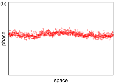
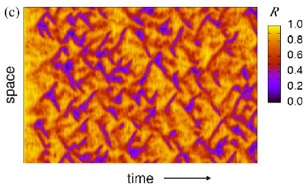
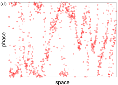
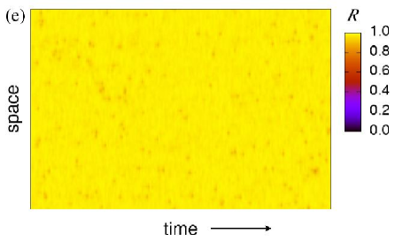
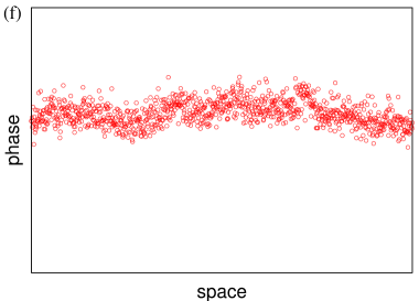
Figure 6: (Color online) Numerical simulations of nonlocally coupled noisy phase oscillators corresponding to the nonlocally coupled noisy Stuart-Landau oscillators for Case SL-I [(a) and (b)], Case SL-II [(c) and (d)], and Case SL-III [(e) and (f)]. (a), (c), and (e): Spatiotemporal patterns of the order parameter modulus. (b), (d), and (f): Instantaneous spatial profile of the local oscillator phase. The number of oscillators is $N=2^{10}$ and the separation between neighboring oscillators is $\varDelta x=0.1$.

Figure 6 displays the numerical results, which correspond to the three cases, SL-I, SL-II, and SL-III, treated in Section II. By comparing Fig. 6 with Fig. 4, we can confirm that the reduced Langevin phase equation nicely reproduces the behavior of the original nonlocally coupled limit-cycle oscillators.

III.4 Nonlinear Fokker-Planck equation

We now transform the Langevin phase equation (14) derived above to an equivalent nonlinear Fokker-Planck equation, which makes the following analysis far easier. To do this, we note that the Langevin phase equation may be viewed as describing the dynamics of a single local oscillator driven by the nonlocal mean field of infinitely many other oscillators sitting within the coupling range. This means that the net coupling force experienced by this local oscillator is a macro-variable, and therefore its statistical fluctuation can be completely negligible. For this reason, the nonlocal coupling term in the phase equation can safely be replaced with its statistical average.

Let us denote by $f(\phi,x,t)$ the probability density function of the phase $\phi$ of a single oscillator at a space-time point $(x,t)$. Following the above argument, we average the coupling term in Eq. (14) by the single-oscillator phase distribution $f(\phi,x,t)$. The equation then takes the form of a single-oscillator Langevin equation driven by a space-time dependent force $V(\phi,x,t)$, that is,

$$\partial_{t}\phi\left(x,t\right)=V\left(\phi,x,t\right)+\sqrt{D}\,\xi\left(x,t\right),$$ (22)

where

$$V\left(\phi,x,t\right)=\omega+\int_{-\infty}^{\infty}dx^{\prime}\,G\left(x-x^{\prime}\right)\int_{0}^{2\pi}d\phi^{\prime}\,\Gamma\left(\phi-\phi^{\prime}\right)f\left(\phi^{\prime},x^{\prime},t\right).$$ (23)

Note that this equation now involves only one dynamical variable, $\phi(x,t)$, as a result of statistical averaging.

The above single-oscillator Langevin equation can be easily transformed to a single-oscillator Fokker-Planck equation in the form ref:risken89 ; ref:gardiner97

$$\frac{\partial f\left(\phi,x,t\right)}{\partial t}=-\frac{\partial}{\partial\phi}\left[\left\{\omega+\int_{-\infty}^{\infty}dx^{\prime}\,G\left(x-x^{\prime}\right)\int_{0}^{2\pi}d\phi^{\prime}\,\Gamma\left(\phi-\phi^{\prime}\right)f\left(\phi^{\prime},x^{\prime},t\right)\right\}f\left(\phi,x,t\right)\right]+D\frac{\partial^{2}f\left(\phi,x,t\right)}{\partial\phi^{2}}.$$ (24)

Since the drift velocity itself involves the distribution $f(\phi,x,t)$, this Fokker-Planck equation is nonlinear. This equation is the starting point for further analysis.

IV Amplitude equation near the onset of collective oscillation

In the following sections, we will further reduce the nonlinear Fokker-Planck equation (24) to analyze its dynamics near the destabilization points. In this section, we first apply the center-manifold reduction to Eq. (24) near the onset of collective oscillations. Following Ref. ref:shiogai03 , we derive the complex Ginzburg-Landau equation, and then present results of numerical simulations that confirm the theoretical conjecture on the noise-induced turbulence.

IV.1 Hopf bifurcation and the complex Ginzburg-Landau equation

The nonlinear Fokker-Planck equation (24) has a trivial constant solution, $f(\phi,x,t)\equiv 1/2\pi$, corresponding to the completely desynchronized state of the oscillators. When the noise intensity $D$ is sufficiently large, this constant solution is stable. As $D$ is decreased, the constant solution is destabilized via a Hopf bifurcation.

In the previous study ref:shiogai03 , it was shown that the nonlinear Fokker-Planck equation (24) has a series of critical noise intensities, below which the system can sustain traveling waves of various wavenumbers. Among them, the spatially uniform oscillating solution of the phase distribution with wavenumber zero has the largest critical noise intensity. Thus, when we decrease $D$ from above, the trivial constant solution gives way to a spatially uniform oscillating solution at a certain critical value $D=D_{c}$.

In the vicinity of this Hopf bifurcation point, we can derive an amplitude equation describing the slow dynamics of the destabilized mode. We introduce a complex amplitude $A(x,t)$ describing the deviation of $f(\phi,x,t)$ from the constant solution $1/2\pi$ as

$$f\left(\phi,x,t\right)=\frac{1}{2\pi}+\frac{1}{2\pi}\Bigl{(}A\left(x,t\right)e^{i\lambda\phi+i\Omega_{c}t}+A^{\ast}\left(x,t\right)e^{-i\lambda\phi-i\Omega_{c}t}\Bigr{)}.$$ (25)

As explained in Ref. ref:shiogai03 , we can derive the complex Ginzburg-Landau equation for this complex amplitude

$$\partial_{t}A\left(x,t\right)=\lambda^{2}\left(D_{c}-D\right)A+d\partial_{x}^{2}A-g\left|A\right|^{2}A,$$ (26)

from the nonlinear Fokker-Planck equation by the center-manifold reduction method ref:kuramoto84 . The parameters of the above complex Ginzburg-Landau equation can be expressed in terms of the Fourier components $\Gamma_{l}$ of the phase coupling function

$$\Gamma(\phi)=\sum_{l=-\infty}^{\infty}\Gamma_{l}\,e^{il\phi}.$$ (27)

As derived in Ref. ref:shiogai03 , they are given by

$$\lambda=\arg\max_{l}\frac{\Im\Gamma_{l}}{l},\quad D_{c}=\frac{\Im\Gamma_{\lambda}}{\lambda},\quad\Omega_{c}=-\lambda\left(\omega+\Re\Gamma_{\lambda}+\Gamma_{0}\right),$$ (28)

$$d=-i\lambda\Gamma_{\lambda},\quad g=\frac{\lambda\Gamma_{\lambda}\left(\Gamma_{2\lambda}+\Gamma_{-\lambda}\right)}{2\Im\Gamma_{\lambda}-i\Re\Gamma_{\lambda}+i\Gamma_{2\lambda}},$$ (29)

where $\Re$ and $\Im$ denote the real part and the imaginary part, respectively. In what follows, we will restrict ourselves to the case of $\lambda=1$ and $\Re g>0$, i.e., the case that the first Fourier component of the phase distribution undergoes a supercritical Hopf bifurcation. This is actually the case with our two representative models of limit-cycle oscillators. When the noise intensity $D$ is decreased below $D_{c}$, Eq. (26) starts to exhibit oscillatory behavior. In this region, by appropriately rescaling the variables, we obtain the standard form of the complex Ginzburg-Landau equation ref:kuramoto84 ; ref:pikovsky01 ; ref:manrubia03 ; ref:cross93 ; ref:bohr98 ; ref:aranson02

$$\partial_{t}A(x,t)=A+(1+ic_{1})\partial_{x}^{2}A-(1+ic_{2})|A|^{2}A,$$ (30)

where the real parameters $c_{1}$ and $c_{2}$ are given by

$$c_{1}=\frac{\Im d}{\Re d},\quad c_{2}=\frac{\Im g}{\Re g}.$$ (31)

We use this standard form in the following discussion.

It is well known that the spatially uniform oscillating solution of the complex Ginzburg-Landau equation becomes unstable and spatiotemporal chaos develops when the Benjamin-Feir instability condition $1+c_{1}c_{2}<0$ is satisfied. Furthermore, it is also known that in the near vicinity of the Benjamin-Feir line, the modulus of the complex Ginzburg-Landau equation tends to be uniform, and the phase component dominates the dynamics of the system. In such a situation, the complex Ginzburg-Landau equation can be further reduced to the Kuramoto-Sivashinsky equation ref:kuramoto84

$$\partial_{t}\Theta(x,t)=-c_{2}+(1+c_{1}c_{2})\partial_{x}^{2}\Theta+(c_{2}-c_{1})(\partial_{x}\Theta)^{2}-\frac{c_{1}^{2}(1+c_{2}^{2})}{2}\partial_{x}^{4}\Theta,$$ (32)

where $\Theta(x,t)$ is the phase of the complex amplitude $A(x,t)$, and is essentially the same as the phase of the order parameter defined in Eq. (10) except for the sign, as we see later. When the Benjamin-Feir instability condition is slightly exceeded, the phase diffusion coefficient $1+c_{1}c_{2}$ of this equation becomes slightly negative, leading to turbulent behavior. In such a case, by an appropriate rescaling of the variables, we obtain the standard form of the Kuramoto-Sivashinsky equation ref:kuramoto84

$$\partial_{t}\Theta(x,t)=-\partial_{x}^{2}\Theta+(\partial_{x}\Theta)^{2}-\partial_{x}^{4}\Theta.$$ (33)

IV.2 Stuart-Landau oscillators

For the sake of simplicity, we treat the nonlocally coupled noisy Stuart-Landau oscillators hereafter. In this case, as seen from Eq. (20) and Eq. (21), the phase coupling function is given by the simple sine function

$$\Gamma\left(\phi\right)=-\sin\left(\phi+\alpha\right),\quad\left|\alpha\right|<\pi/2,$$ (34)

which is the in-phase type coupling. The parameters of the reduced complex Ginzburg-Landau equation can be calculated as

$$D_{c}=\frac{\cos\alpha}{2},\quad c_{1}=\frac{\Im d}{\Re d}=\tan\alpha,\quad c_{2}=\frac{\Im g}{\Re g}=-\frac{\tan\alpha}{2}.$$ (35)

By choosing the parameter $\alpha$ appropriately, the Benjamin-Feir instability condition can be satisfied. Thus, it was conjectured in Refs. ref:shiogai03 ; ref:kuramoto06 that, since the reduced complex Ginzburg-Landau equation can exhibit turbulent behavior, the corresponding nonlinear Fokker-Planck equation, the Langevin phase equation, and the original nonlocally coupled noisy limit-cycle oscillators, could also exhibit turbulent behavior under suitable conditions.

To examine this conjecture, we conduct systematic numerical simulations near the Hopf bifurcation curve.

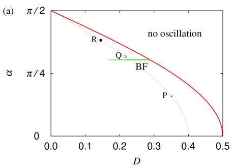
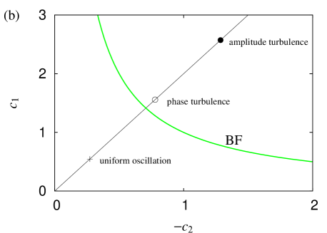
Figure 7: (Color online) (a): Phase diagram plotted as a function of the noise intensity $D$ and the phase shift $\alpha$. The red solid curve represents the Hopf bifurcation line ($D=D_{c}=\cos(\alpha)/2$). For numerical simulations near the bifurcation, the noise intensity is chosen such that $D/D_{c}=0.8$ indicated by the dotted curve. The Benjamin-Feir (BF) critical line ($\alpha=\arctan\sqrt{2}$) is also indicated. (b): Phase diagram plotted as a function of the parameters $c_{1}=\Im d/\Re d=\tan(\alpha)$ and $c_{2}=\Im g/\Re g=-\tan(\alpha)/2$. Plus (Case P: $\alpha=0.5,D/D_{c}=0.8$), open circle (Case Q: $\alpha=1.0,D/D_{c}=0.8$), and filled circle (Case R: $\alpha=1.2,D/D_{c}=0.8$) correspond to spatially uniform oscillation, phase turbulence, and amplitude turbulence, respectively. The Benjamin-Feir (BF) line ($1+c_{1}c_{2}=0$) is also indicated by the green curve.

Theoretical bifurcation diagrams of the complex Ginzburg-Landau equation are plotted as a function of the parameters $\alpha$ and $D$ in Fig. 7(a), and as a function of the parameters $c_{1}$ and $c_{2}$ in Fig. 7(b). The red solid line in Fig. 7(a) represents the Hopf bifurcation curve, below which the complex amplitude $A(x,t)$ starts to oscillate. In the numerical simulations, we fix the noise intensity at $D/D_{c}=0.8$, which corresponds to the black line. We choose three representative points on this line, indicated by P, Q, and R. The green line represents the Benjamin-Feir instability curve $1+c_{1}c_{2}=0$, which can be expressed as $\alpha=\arctan\sqrt{2}$ from Eq. (35).

Note that the parameters $c_{1}$ and $c_{2}$ cannot change independently in the present model. From Eq. (35), only pairs of $(c_{1},c_{2})$ satisfying $c_{1}=-2c_{2}$ drawn as the straight line in Fig. 7(b) can be realized. The three representative cases P, Q, and R correspond to three different dynamical states of the complex Ginzburg-Landau equation, namely, spatially uniform oscillation, phase turbulence, and amplitude turbulence, respectively ref:shraiman92 . On these points, we numerically simulate the Langevin phase equation and the corresponding nonlinear Fokker-Planck equation (and, in some cases, also the complex Ginzburg-Landau equation and the Kuramoto-Sivashinsky equation). Numerical methods used in the simulations are summarized in Appendix C. In drawing the figures presented hereafter, numerical results obtained from the different equations are appropriately rescaled to accord with the standard form of the complex Ginzburg-Landau equation (30) or the Kuramoto-Sivashinsky equation (33).

	(a)	(b)
time $\rightarrow$

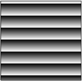
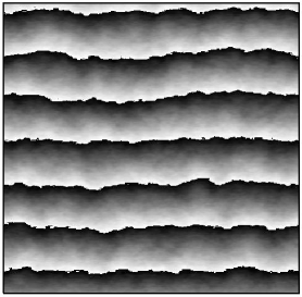
Figure 8: Uniform oscillation. Parameter values are $\alpha=0.5$ and $D/D_{c}=0.8$ (Case P). Space (horizontal)-time (vertical) plot of order parameter phase $\Theta(x,t)$ for Fokker-Planck simulation (a) and Langevin simulation using $N=2^{15}$ oscillators (b).

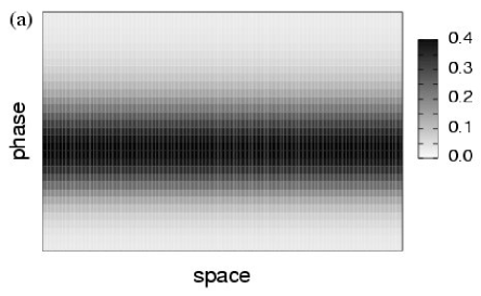
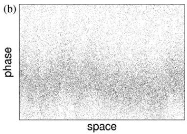
Figure 9: Uniform oscillation. Parameter values are $\alpha=0.5$ and $D/D_{c}=0.8$ (Case P). (a): Instantaneous spatial profile of phase distribution function obtained from Fokker-Planck simulation. (b): Instantaneous spatial profile of local oscillator phase obtained from Langevin simulation using $N=2^{15}$ oscillators.

Figures 8 and 9 display the results at the parameter point P, where we expect stable uniform oscillation obtained by direct numerical simulations of the nonlinear Fokker-Planck equation (24) and the Langevin phase equation (14). Figures 8(a) and 8(b) plot the temporal evolution of the order parameter phase $\Theta(x,t)$ defined in Eq. (10). As expected from the phase diagram of the reduced complex Ginzburg-Landau equation, both equations exhibit spatially uniform oscillating solutions. Small non-uniformity seen in the Langevin simulation, Fig. 8(b), is due to trivial statistical fluctuations. Figures 9(a) and Fig. 9(b) display the snapshots of the instantaneous spatial distribution of the phases. We can confirm that the phase distributions are spatially uniform.

	(a)	(b)	(c)
time $\rightarrow$

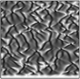
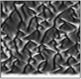
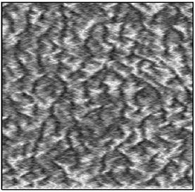
Figure 10: Amplitude turbulence. Parameter values are $\alpha=1.2$ and $D/D_{c}=0.8$ (Case R). Space (horizontal) - time (vertical) plot of the order parameter modulus $R(x,t)$ is shown in rescaled units with which the complex Ginzburg-Landau equation takes the standard form, Eq. (30), whose system size is $L\simeq 114$. Numerical data obtained form the complex Ginzburg-Landau equation (a), the nonlinear Fokker-Planck equation (b), and the Langevin phase equation using $N=2^{15}$ oscillators (c) are compared.

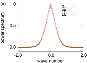
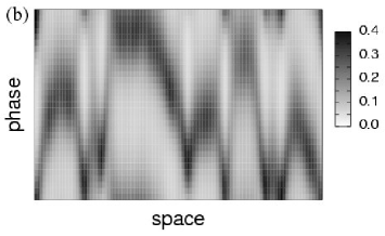
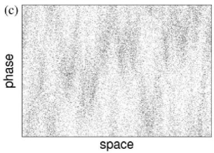
Figure 11: (Color online) Amplitude turbulence. Parameter values are $\alpha=1.2$ and $D/D_{c}=0.8$ (Case R). (a): Spatial power spectrum of the order parameter as a function of the wavenumber in rescaled units with which the complex Ginzburg-Landau equation takes the standard form, Eq. (30). Numerical data obtained from the complex Ginzburg-Landau equation (GL), the nonlinear Fokker-Planck equation (FP), and the Langevin phase equation (LE) are compared. (b): Instantaneous spatial profile of the phase distribution function obtained from the Fokker-Planck simulation. (c): Instantaneous spatial profile of the local oscillator phase obtained from the Langevin simulation using $N=2^{15}$ oscillators.

Numerical results obtained at the parameter point R, where the amplitude turbulence is expected in the reduced complex Ginzburg-Landau equation, are shown in Figs. 10 and 11. Figures 10(a), 10(b), and 10(c) show spatiotemporal patterns of the modulus $R(x,t)$ of the order parameter defined in Eq. (10), obtained by numerical simulations of the complex Ginzburg-Landau equation, the nonlinear Fokker-Planck equation, and the Langevin phase equation, respectively. As mentioned above, the order parameter defined in Eq. (10) gives the first Fourier mode of the phase distribution, which corresponds to the complex conjugation of the complex amplitude for the reduced complex Ginzburg-Landau equation as

$$R\left(x,t\right)e^{i\Theta\left(x,t\right)} \equiv\int^{\infty}_{-\infty}dx^{\prime}\,G\left(x-x^{\prime}\right)e^{i\phi\left(x^{\prime},t\right)}$$ (36)

$$=\int^{\infty}_{-\infty}dx^{\prime}\,G\left(x-x^{\prime}\right)\int^{2\pi}_{0}d\phi^{\prime}\,e^{i\phi^{\prime}}f\left(\phi^{\prime},x^{\prime},t\right)$$ (37)

$$=\int^{\infty}_{-\infty}dx^{\prime}\,G\left(x-x^{\prime}\right)A^{\ast}\left(x^{\prime},t\right)e^{-i\Omega_{c}t}$$ (38)

$$\simeq A^{\ast}\left(x,t\right)e^{-i\Omega_{c}t},$$ (39)

where we used the fact that the characteristic wavelength becomes sufficiently longer than the length of the the nonlocal coupling near the critical point in the last approximation. The three patterns are quite similar to each other. Figure 11(a) shows the spatial power spectrum of the order parameter. They are also almost identical to each other. Figures 11(b) and 11(c) show the snapshots of the phase distributions obtained from the nonlinear Fokker-Planck equation and the Langevin phase equation, respectively. In both figures, we can observe strongly nonuniform phase distributions due to turbulent fluctuations, which again resemble with each other. These results clearly indicate that the turbulent fluctuations exhibited by the three equations are generated by the same dynamical instability.

	(a)	(b)	(c)
time $\rightarrow$

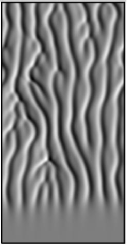
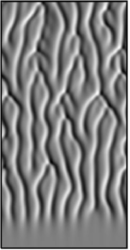
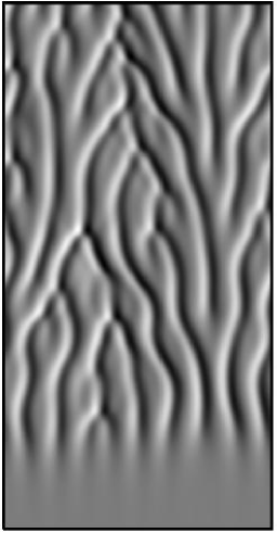
Figure 12: Phase turbulence. Parameter values are $\alpha=1.0$ and $D/D_{c}=0.8$ (Case Q). Space (horizontal) - time (vertical) plot of the order parameter phase gradient $v(x,t)=2\partial_{x}\Theta(x,t)$ is shown in rescaled units with which the Kuramoto-Sivashinsky equation takes the standard form, Eq. (33), whose system size is $L\simeq 76$. Numerical data obtained from the Kuramoto-Sivashinsky equation (a), the complex Ginzburg-Landau equation (b), and the nonlinear Fokker-Planck equation (c) are compared.

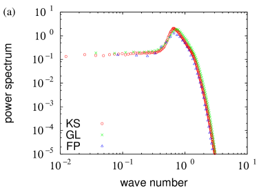
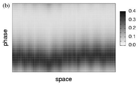
Figure 13: (Color online) Phase turbulence. Parameter values are $\alpha=1.0$ and $D/D_{c}=0.8$ (Case Q). (a): Spatial power spectrum of the order parameter phase gradient $v(x,t)=2\partial_{x}\Theta(x,t)$ is plotted as a function of the wavenumber in rescaled units with which the Kuramoto-Sivashinsky equation takes the standard form, Eq. (33). Numerical data obtained from the Kuramoto-Sivashinsky equation (KS), the complex Ginzburg-Landau equation (GL), and the nonlinear Fokker-Planck equation (FP) are compared. (b): Instantaneous spatial profile of the phase distribution function obtained from the Fokker-Planck simulation.

Finally, the numerical results for the parameter Q, for which phase turbulence is expected, are shown in Figs. 12 and 13. Figure 12 compares the results from the Kuramoto-Sivashinsky equation, the complex Ginzburg-Landau equation, and the nonlinear Fokker-Planck equation, where the spatiotemporal evolution of the phase gradient $v(x,t)=2\partial_{x}\Theta(x,t)$ of the order parameter is plotted for each equation. They are remarkably similar to each other. In Fig. 13(a), spatial power spectrum of the order parameter phase gradient is plotted for each equation. They also show excellent agreement with each other. Figure 13(b) shows a snapshot of the phase distribution function obtained from the nonlinear Fokker-Planck equation. As expected, long-wavelength phase fluctuations are observed.

These numerical results confirm the existence of the noise-induced transition from the constant solution via the Hopf bifurcation and the Benjamin-Feir instability.

V Phase equation near the destabilization point of the spatially uniform oscillation

In the previous section, we have analyzed the nonlinear Fokker-Planck equation near the Hopf bifurcation point of the constant solution using the center-manifold reduction. In this section, we investigate a different parameter region, where the uniformly oscillating solution of the nonlinear Fokker-Planck equation loses its stability against phase disturbances. As a result, a transition line to the spatiotemporal chaos will be determined, which completes the phase diagram of the noise-induced turbulence.

V.1 Lower transition line to the spatiotemporal chaos

In the previous section, it was found that the constant solution of the nonlinear Fokker-Planck equation, which is stable for large noise intensity, loses its stability via the supercritical Hopf bifurcation as the noise intensity is decreased, and the order parameter exhibits spatiotemporal chaos near the Hopf bifurcation point under suitable conditions. However, the spatially uniform oscillating solution of all the oscillators is stable in the absence of noise, since we assume the in-phase coupling in the original nonlocally coupled limit-cycle oscillators. Thus, there should be a lower critical noise intensity, above which the uniformly oscillating solution of the oscillators loses its stability and gives way to the spatiotemporal chaos.

Figure 14: Schematic phase diagram of the noise-induced turbulence as a function of the phase shift $\alpha$ and the noise intensity $D$.

The schematic phase diagram which describes this situation is illustrated in Fig. 14. Below we analyze the situation where the order parameter becomes turbulent as the noise intensity is increased from zero. We use the method of phase reduction once again to derive a phase equation describing the dynamics of slowly varying wavefronts.

V.2 Slow phase modulation of the spatially uniform oscillation

We here give the outline of the analysis. Details of the analytical calculations are given in Appendix B. First, we focus on the spatially uniform oscillating solution $f_{0}(\theta-\Theta_{0})$ of the nonlinear Fokker-Planck equation, where $\theta=\phi-\Omega t$. Here, $\Omega$ is the frequency of the collective oscillation, and the constant $\Theta_{0}$ is the initial phase that can be chosen arbitrary. We then allow this phase constant $\Theta_{0}$ to be slowly space-time dependent, and denote it as $\Theta(x,t)$.

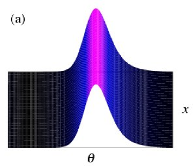
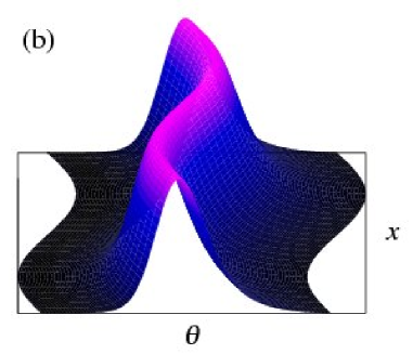
Figure 15: (Color online) Schematic phase distribution function $f_{0}(\theta-\Theta)$ with a spatially uniform phase, $\Theta=\Theta_{0}$ (a), and with a spatially slowly varying phase, $\Theta=\Theta(x,t)$ (b).

Figure 15(a) shows a schematic picture of a spatially uniform oscillating solution, whose order parameter phase $\Theta_{0}$ is constant, and Fig. 15(b) the case that the order parameter phase $\Theta(x,t)$ is slowly varying. The phase of the slowly modulated oscillating solution defined here is essentially the same as the phase of the order parameter defined previously in Eq. (10) except for the mean drift term $\Omega t$, as long as the spatial scale of the variation is sufficiently long compared to the coupling length. Thus, we use the same notation $\Theta(x,t)$ for both phase variables. As shown in Appendix B, we can derive an equation for the phase $\Theta(x,t)$ in a closed form using the analytical procedure given in Ref. ref:kuramoto84 . If we truncate the series of gradient expansion retaining the first few terms, the derived phase equation has the form

$$\partial_{t}\Theta\left(x,t\right)=\bar{\nu}\partial_{x}^{2}\Theta+\bar{\mu}\left(\partial_{x}\Theta\right)^{2}-\bar{\lambda}\partial_{x}^{4}\Theta+\cdot\cdot\cdot,$$ (40)

where the parameters $\bar{\nu}$, $\bar{\mu}$, and $\bar{\lambda}$ can be calculated using the phase coupling function $\Gamma(\phi)$, the spatially uniform oscillating solution $f_{0}(\theta)$, and its associated left- and right eigenfunctions. Among these parameters, the phase diffusion coefficient $\bar{\nu}$ is the most important quantity. When $\bar{\nu}$ changes its sign from positive to negative, the spatially uniform oscillating solution loses its stability, and spatiotemporal chaos sets in.

V.3 Phase diagram for the Stuart-Landau case

For the case of the Stuart-Landau oscillators with the phase coupling function given in Eq. (34), we numerically calculated the phase diffusion coefficient $\bar{\nu}$ at various values of the phase shift $\alpha$ and the noise intensity $D$, and determined the $\bar{\nu}=0$ curve on the $\alpha$-$D$ plane.

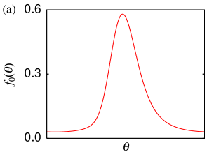
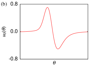
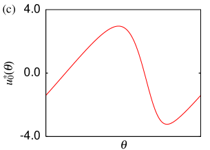
Figure 16: (Color online) Numerically obtained spatially uniform oscillating solution (a), right zero eigenfunction (b), and left zero eigenfunction (c). The parameter values are $\alpha=1.2$ and $D/D_{c}=0.5$, which give $\bar{\nu}\simeq-0.371652.$

Typical functional shapes of $f_{0}(\theta)$, $u_{0}(\theta)$, and $u_{0}^{\ast}(\theta)$ obtained from the numerical calculations are illustrated in Fig. 16.

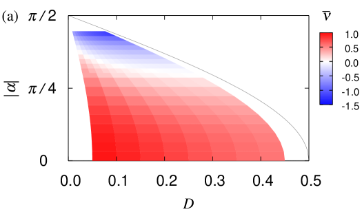
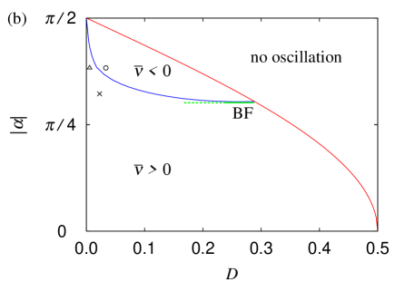
Figure 17: (Color online) Dependence of the phase diffusion coefficient $\bar{\nu}$ on the phase shift $\alpha$ and the noise intensity $D$. (a): $\bar{\nu}$ was numerically evaluated in the parameter region with $\alpha\in[0.0,1.4]$ and $D/D_{c}\in[0.1,0.9]$. $\bar{\nu}$ is negative in the blue region, and positive in the red region. (b): The red and blue curves represent the Hopf bifurcation line ($D=D_{c}$) and the noise-induced transition line to turbulent state ($\bar{\nu}=0$). The Benjamin-Feir (BF) line is also indicated by the green line. Cases SL-I, SL-II, and SL-III are indicated by the triangle, the open circle, and the cross, respectively.

In Fig. 17(a), dependence of the phase diffusion coefficient $\bar{\nu}$ on $\alpha$ and $D$ is illustrated. $\bar{\nu}$ is positive in the red region, and negative in the blue region. Figure 17(b) represents the whole phase diagram. The blue curve represents $\bar{\nu}=0$. The red line represents the Hopf bifurcation curve, and the green line the Benjamin-Feir criticality near the Hopf bifurcation. In the parameter region surrounded by the red curve and the blue curve, the phase diffusion coefficient $\bar{\nu}$ is negative, indicating that spatiotemporal chaos appears in this region. The Benjamin-Feir criticality line, which we obtained in the previous section by the center-manifold reduction, is also consistent with the results of the present phase reduction analysis.

Let us now look back on the numerical results of the original nonlocally coupled noisy Stuart-Landau oscillators (Fig. 4) and also its reduced phase model (Fig. 6). Three sets of the parameters used in Fig. 4 and 6, SL-I, SL-II, and SL-III, are also plotted on the phase diagram in Fig. 17(b). As can be seen, only the case SL-II is in the region of noise-induced turbulent states. The other two cases, SL-I and SL-III, are in the parameter region where the spatially uniform oscillation is stable. Thus, our theory consistently explains the occurrence of noise-induced turbulence.

VI Concluding Remarks

We studied a system of nonlocally coupled limit-cycle oscillators subject to spatiotemporal white Gaussian noise, which exhibits a remarkable phenomenon called noise-induced turbulence. We considered the case that the coupling and the noise are sufficiently weak, and reduced the system to nonlocally coupled noisy phase oscillators by using the phase reduction method. We then derived an equivalent nonlinear Fokker-Planck equation from the Langevin phase equation, utilizing the fact that the mean-field theory exactly holds owing to the nonlocal coupling. The center-manifold reduction was applied to the situation where the trivial constant solution of the nonlinear Fokker-Planck equation becomes unstable and starts to oscillate, and we derived the complex Ginzburg-Landau equation. Furthermore, we also derived the Kuramoto-Sivashinsky-type equation from the nonlinear Fokker-Planck equation by applying the phase reduction method once again.

Table 1: Hierarchy of equations for noise-induced turbulence.

The hierarchy of our equations derived for the noise-induced turbulence is summarized in Table. 1. Our theoretical analysis and numerical simulations thus provide strong evidence for the existence of noise-induced turbulence in systems of nonlocally coupled noisy limit-cycle oscillators.

Finally, we briefly discuss how to distinguish the noise-induced effective deterministic dynamics of the system from the noisy patterns when the precise dynamical equation describing the system is not available. In principle, we will be able to detect the bifurcations of the effective deterministic dynamics, if appropriately filtered spatial patterns exhibit qualitative changes as the external noise intensity is varied. For our nonlocally coupled noisy oscillators, we introduced the space-time dependent complex order parameter given by Eq. (10) to observe the effective deterministic dynamics of the system, where the nonlocal coupling function $G(x)$ was used as the kernel function that filters the noisy patterns to eliminate nonessential statistical fluctuations. For experimental systems, however, there would be cases that the appropriate kernel function is not known in advance and should be determined empirically. The precise form of the kernel function is not important, so that the essential parameter is the width of the kernel function, namely, the coarse-graining scale of the noisy patterns. One possible method to estimate the appropriate width of the kernel function is to utilize a spatial correlation function $C(x)$ of the local oscillators at a sufficiently strong noise intensity, where no collective oscillations arises. The correlation length of $C(x)$ calculated in such a regime will directly reflect the coupling length of the system, which gives a reasonable estimate of the appropriate kernel width. We can then filter the noisy patterns using a suitable localized kernel function, such as the Gaussian or the exponential kernel, whose width is given by the obtained correlation length. For our nonlocally coupled oscillators, the correlation length of $C(x)$ directly reflects the coupling length of $G(x)$. Using the method explained above, we could actually observe spatiotemporal patterns similar to those observed using the complex order parameter, Eq. (10), without assuming prior knowledge of the nonlocal coupling function $G(x)$.

We believe that noise-induced turbulence can be experimentally realized in the near future.

Appendix A Phase reduction of coupled noisy limit-cycle oscillators

We consider the following Langevin equation describing an ensemble of coupled identical limit-cycle oscillators subject to independent noises

$$\partial_{t}\mbox{\boldmath$X$}_{n}\left(t\right)=\mbox{\boldmath$F$}\left(\mbox{\boldmath$X$}_{n}\right)+\sum_{n^{\prime}}\mbox{\boldmath$V$}_{n,n^{\prime}}\left(\mbox{\boldmath$X$}_{n},\mbox{\boldmath$X$}_{n^{\prime}}\right)+\sqrt{\sigma}\,\mbox{\boldmath$\eta$}_{n}\left(t\right),$$ (41)

where $\mbox{\boldmath$X$}_{n}(t)$ represents the state of the $n$-th oscillator at time $t$, $\mbox{\boldmath$F$}(\mbox{\boldmath$X$}_{n})$ the individual dynamics, $\mbox{\boldmath$V$}_{n,n^{\prime}}(\mbox{\boldmath$X$}_{n},\mbox{\boldmath$X$}_{n^{\prime}})$ the interaction between $n$- and $n^{\prime}$-th oscillators, $\sigma$ the noise intensity, and $\mbox{\boldmath$\eta$}_{n}(t)$ the external noise added independently to each oscillator. The noise $\mbox{\boldmath$\eta$}_{n}(t)$ is assumed to be white Gaussian, whose statistics are given by

$$\left\langle\eta^{j}_{n}\left(t\right)\right\rangle=0,\quad\left\langle\eta^{j}_{n}\left(t\right)\eta^{j^{\prime}}_{n^{\prime}}\left(t^{\prime}\right)\right\rangle=2\delta_{j,j^{\prime}}\delta_{n,n^{\prime}}\delta\left(t-t^{\prime}\right),$$ (42)

where the superscripts $j$ and $j^{\prime}$ denote the vector component. When the coupling term and the noise term are sufficiently small, the phase reduction method is applicable. Applying the phase reduction method ref:kuramoto84 , we obtain the following Langevin equation for the phase variables:

$$\partial_{t}\phi_{n}\left(t\right)=\omega+\sum_{n^{\prime}}\mbox{\boldmath$Z$}\left(\phi_{n}\right)\cdot\mbox{\boldmath$V$}_{n,n^{\prime}}\left(\phi_{n},\phi_{n^{\prime}}\right)+\sqrt{\sigma}\mbox{\boldmath$Z$}\left(\phi_{n}\right)\cdot\mbox{\boldmath$\eta$}_{n}\left(t\right).$$ (43)

Here, $\omega$ is the natural frequency of the oscillators, $\mbox{\boldmath$Z$}(\phi_{n})$ is the phase sensitivity function ref:kuramoto84 , and $\mbox{\boldmath$V$}_{n,n^{\prime}}(\phi_{n},\phi_{n^{\prime}})$ is the abbreviation of $\mbox{\boldmath$V$}_{n,n^{\prime}}(\mbox{\boldmath$X$}_{0}(\phi_{n}),\mbox{\boldmath$X$}_{0}(\phi_{n^{\prime}}))$, where $\mbox{\boldmath$X$}_{0}$ is the unperturbed limit-cycle solution. By virtue of the independent Gaussian statistics, we can rewrite the above equation (43) in the following form

$$\partial_{t}\phi_{n}\left(t\right)=\omega+\sum_{n^{\prime}}\mbox{\boldmath$Z$}\left(\phi_{n}\right)\cdot\mbox{\boldmath$V$}_{n,n^{\prime}}\left(\phi_{n},\phi_{n^{\prime}}\right)+\sqrt{\sigma}\left\|\mbox{\boldmath$Z$}\left(\phi_{n}\right)\right\|\xi_{n}\left(t\right),$$ (44)

where $\|\mbox{\boldmath$Z$}(\phi_{n})\|=\sqrt{\mbox{\boldmath$Z$}(\phi_{n})\cdot\mbox{\boldmath$Z$}(\phi_{n})}$ and the statistics of the white Gaussian noise $\xi_{n}$ is given by

$$\left\langle\xi_{n}\left(t\right)\right\rangle=0,\quad\left\langle\xi_{n}\left(t\right)\xi_{n^{\prime}}\left(t^{\prime}\right)\right\rangle=2\delta_{n,n^{\prime}}\delta\left(t-t^{\prime}\right).$$ (45)

We introduce the new slow phase variables $\bar{\phi}_{n}$ as

$$\phi_{n}=\omega t+\bar{\phi}_{n},$$ (46)

and rewrite the above Langevin equation (44) as

$$\partial_{t}\bar{\phi}_{n}\left(t\right)=\sum_{n^{\prime}}\mbox{\boldmath$Z$}\left(\omega t+\bar{\phi}_{n}\right)\cdot\mbox{\boldmath$V$}_{n,n^{\prime}}\left(\omega t+\bar{\phi}_{n},\omega t+\bar{\phi}_{n^{\prime}}\right)+\sqrt{\sigma}\left\|\mbox{\boldmath$Z$}\left(\omega t+\bar{\phi}_{n}\right)\right\|\xi_{n}\left(t\right).$$ (47)

The corresponding Fokker-Planck equation describing the evolution of the probability density function $P(\{\bar{\phi}_{n}\},t)$ of the phase variables is given by

$$\frac{\partial}{\partial t}P\left(\{\bar{\phi}_{n}\},t\right)=\sum_{n}\left(-\frac{\partial}{\partial\bar{\phi}_{n}}\right)J_{n}\left(\{\bar{\phi}_{n}\},t\right),$$ (48)

where

$$J_{n}\left(\{\bar{\phi}_{n}\},t\right) =\left[\sum_{n^{\prime}}\mbox{\boldmath$Z$}\left(\omega t+\bar{\phi}_{n}\right)\cdot\mbox{\boldmath$V$}_{n,n^{\prime}}\left(\omega t+\bar{\phi}_{n},\omega t+\bar{\phi}_{n^{\prime}}\right)+\frac{1}{2}\frac{\partial}{\partial\bar{\phi}_{n}}\Bigl{(}\sigma\left\|\mbox{\boldmath$Z$}(\omega t+\bar{\phi}_{n})\right\|^{2}\Bigr{)}\right]P\left(\{\bar{\phi}_{n}\},t\right)$$

$$-\frac{\partial}{\partial\bar{\phi}_{n}}\Biggl{[}\sigma\left\|\mbox{\boldmath$Z$}(\omega t+\bar{\phi}_{n})\right\|^{2}P\left(\{\bar{\phi}_{n}\},t\right)\Biggr{]}.$$ (49)

Rapidly oscillating quantities in $J_{n}(\{\bar{\phi}_{n}\},t)$ are now time averaged over one period of the oscillator. The resulting averaged Fokker-Planck equation has the following form

$$\frac{\partial}{\partial t}P\left(\{\bar{\phi}_{n}\},t\right)=\sum_{n}\left(-\frac{\partial}{\partial\bar{\phi}_{n}}\right)\left(\sum_{n^{\prime}}\Gamma_{n,n^{\prime}}\left(\bar{\phi}_{n}-\bar{\phi}_{n^{\prime}}\right)P\left(\{\bar{\phi}_{n}\},t\right)-D\frac{\partial}{\partial\bar{\phi}_{n}}P\left(\{\bar{\phi}_{n}\},t\right)\right),$$ (50)

where the phase coupling function $\Gamma_{n,n^{\prime}}(\bar{\phi}_{n}-\bar{\phi}_{n^{\prime}})$ is given by

$$\Gamma_{n,n^{\prime}}\left(\bar{\phi}_{n}-\bar{\phi}_{n^{\prime}}\right)=\frac{1}{2\pi}\int_{0}^{2\pi}d\lambda\;\mbox{\boldmath$Z$}\left(\lambda+\bar{\phi}_{n}\right)\cdot\mbox{\boldmath$V$}_{n,n^{\prime}}\left(\lambda+\bar{\phi}_{n},\lambda+\bar{\phi}_{n^{\prime}}\right),$$ (51)

and also the effective noise intensity $D$ is given by

$$D=\frac{1}{2\pi}\int_{0}^{2\pi}d\lambda\;\sigma\mbox{\boldmath$Z$}\left(\lambda+\bar{\phi}_{n}\right)\cdot\mbox{\boldmath$Z$}\left(\lambda+\bar{\phi}_{n}\right).$$ (52)

The Langevin equation corresponding to the averaged Fokker-Planck equation (50) is expressed as

$$\partial_{t}\bar{\phi}_{n}\left(t\right)=\sum_{n^{\prime}}\Gamma_{n,n^{\prime}}\left(\bar{\phi}_{n}-\bar{\phi}_{n^{\prime}}\right)+\sqrt{D}\,\xi_{n}\left(t\right).$$ (53)

Finally, we obtain the following Langevin equation for the phases:

$$\partial_{t}\phi_{n}\left(t\right)=\omega+\sum_{n^{\prime}}\Gamma_{n,n^{\prime}}\left(\phi_{n}-\phi_{n^{\prime}}\right)+\sqrt{D}\,\xi_{n}\left(t\right).$$ (54)

Now let us consider the nonlocally coupled oscillator system. The above formulae can be written in the form

$$\sum_{n^{\prime}}\mbox{\boldmath$V$}_{n,n^{\prime}}\left(\mbox{\boldmath$X$}_{n},\mbox{\boldmath$X$}_{n^{\prime}}\right) \to\int dx^{\prime}\,G\left(x-x^{\prime}\right)\mbox{\boldmath$V$}\left(\mbox{\boldmath$X$},\mbox{\boldmath$X$}^{\prime}\right),$$ (55)

$$\sum_{n^{\prime}}\Gamma_{n,n^{\prime}}\left(\phi_{n}-\phi_{n^{\prime}}\right) \to\int dx^{\prime}\,G\left(x-x^{\prime}\right)\Gamma\left(\phi-\phi^{\prime}\right),$$ (56)

where

$$\Gamma\left(\phi-\phi^{\prime}\right)=\frac{1}{2\pi}\int_{0}^{2\pi}d\lambda\;\mbox{\boldmath$Z$}\left(\lambda+\phi\right)\cdot\mbox{\boldmath$V$}\left(\lambda+\phi,\lambda+\phi^{\prime}\right).$$ (57)

Here, $\mbox{\boldmath$X$}^{\prime}$ and $\phi^{\prime}$ are the abbreviations of $\mbox{\boldmath$X$}(x^{\prime},t)$ and $\phi(x^{\prime},t)$, respectively.

Appendix B Second phase reduction of the nonlinear Fokker-Planck equation

In this appendix, we present analytical procedures to derive a phase equation describing the slow phase modulation of the spatially uniform oscillating solution. We assume long-wavelength modulation to the spatially uniform oscillation, so that the spatial derivatives of the function $f(\phi,x,t)$ are small quantities. We thus expand the nonlocal coupling term of the Fokker-Planck equation as

$$\int_{-\infty}^{\infty}dx^{\prime}\,G\left(x-x^{\prime}\right)f\left(\phi,x^{\prime},t\right)=\sum_{m=0}^{\infty}G_{2m}\,\partial_{x}^{2m}f\left(\phi,x,t\right),$$ (58)

where $G_{2m}$ is the $2m$-th moment of $G(x)$. It is given by $G_{2m}=\int_{-\infty}^{\infty}dx\,G(x)x^{2m}/(2m)!$, where $G_{0}=1$ holds from the normalization condition. Due to the spatial reflection symmetry, only even moments $G_{2m}$ remain. For the coupling function used in this paper, $G(x)=\exp(-|x|)/2$, we obtain $G_{2m}=1$ for all $m$. The nonlinear Fokker-Planck equation is expanded as

$$\frac{\partial f(\phi,x,t)}{\partial t}= -\frac{\partial}{\partial\phi}\left[\left\{\omega+\int_{0}^{2\pi}d\phi^{\prime}\,\Gamma\left(\phi-\phi^{\prime}\right)f\left(\phi^{\prime},x,t\right)\right\}f\left(\phi,x,t\right)\right]+D\frac{\partial^{2}f(\phi,x,t)}{\partial\phi^{2}}$$

$$-\frac{\partial}{\partial\phi}\left[\int_{0}^{2\pi}d\phi^{\prime}\,\Gamma\left(\phi-\phi^{\prime}\right)\Bigl{\{}G_{2}\partial_{x}^{2}f\left(\phi^{\prime},x,t\right)\Bigr{\}}f\left(\phi,x,t\right)\right]$$

$$-\frac{\partial}{\partial\phi}\left[\int_{0}^{2\pi}d\phi^{\prime}\,\Gamma\left(\phi-\phi^{\prime}\right)\Bigl{\{}G_{4}\partial_{x}^{4}f\left(\phi^{\prime},x,t\right)\Bigr{\}}f\left(\phi,x,t\right)\right]$$

$$-\cdot\cdot\cdot.$$ (59)

Let us denote by $f(\phi,x,t)=f_{0}(\theta)=f_{0}(\phi-\Omega t)$ the spatially uniform oscillating solution of the nonlinear Fokker-Planck equation, where $\Omega$ is the collective frequency. Inserting this expression in the nonlinear Fokker-Planck equation, we find that $f_{0}(\theta)$ satisfies the following equation

$$D\frac{d^{2}}{d\theta^{2}}f_{0}\left(\theta\right)+\left(\Omega-\omega\right)\frac{d}{d\theta}f_{0}\left(\theta\right)-\frac{d}{d\theta}\Bigl{[}g_{0}\left(\theta\right)f_{0}\left(\theta\right)\Bigr{]}=0,$$ (60)

where

$$g_{0}\left(\theta\right)=\int_{0}^{2\pi}d\theta^{\prime}\,\Gamma\left(\theta-\theta^{\prime}\right)f_{0}\left(\theta^{\prime}\right).$$ (61)

Let $u(\theta,t)$ represent disturbance to the spatially uniform oscillating solution defined by $f(\phi,x,t)=f_{0}(\theta)+u(\theta,t)$. Eq. (59) is linearized in $u(\theta,t)$, i.e., $\partial_{t}u=\hat{L}u$, where the linearized operator $\hat{L}$ is defined as

$$\hat{L}u=D\frac{d^{\,2}}{d\theta^{2}}u\left(\theta\right)+\left(\Omega-\omega\right)\frac{d}{d\theta}u\left(\theta\right)-\frac{d}{d\theta}\Bigl{[}g_{0}\left(\theta\right)u\left(\theta\right)\Bigr{]}-\frac{d}{d\theta}\left[f_{0}\left(\theta\right)\int_{0}^{2\pi}d\theta^{\prime}\,\Gamma\left(\theta-\theta^{\prime}\right)u\left(\theta^{\prime}\right)\right],$$ (62)

whose adjoint operator $\hat{L}^{\ast}$, defined by $\int_{0}^{2\pi}d\theta\,u^{\ast}(\theta)\hat{L}u(\theta)=\int_{0}^{2\pi}d\theta\,u(\theta)\hat{L}^{\ast}u^{\ast}(\theta)$, is expressed as

$$\hat{L}^{\ast}u^{\ast}=D\frac{d^{\,2}}{d\theta^{2}}u^{\ast}\left(\theta\right)-\left(\Omega-\omega\right)\frac{d}{d\theta}u^{\ast}\left(\theta\right)+g_{0}\left(\theta\right)\frac{d}{d\theta}u^{\ast}\left(\theta\right)+\int_{0}^{2\pi}d\theta^{\prime}\,\Gamma\left(\theta^{\prime}-\theta\right)f_{0}\left(\theta^{\prime}\right)\frac{d}{d\theta^{\prime}}u^{\ast}\left(\theta^{\prime}\right).$$ (63)

The left- and the right eigenfunctions and their eigenvalues of these linear operators are determined from

$$\hat{L}u_{l}=\lambda_{l}u_{l},\quad\hat{L}^{\ast}u_{l}^{\ast}=\lambda_{l}u_{l}^{\ast}\quad\left(l=0,1,2,\cdot\cdot\cdot\right).$$ (64)

The eigenfunctions are assumed to be orthonormalized as

$$\int_{0}^{2\pi}d\theta\,u_{l}^{\ast}\left(\theta\right)u_{m}\left(\theta\right)=\delta_{lm}.$$ (65)

Here we should note that the right zero eigenfunction can be chosen as

$$\hat{L}u_{0}=0,\quad u_{0}\left(\theta\right)=\frac{d}{d\theta}f_{0}\left(\theta\right),\quad\lambda_{0}=0,$$ (66)

which follows from the differentiation of Eq. (60) with respect to $\theta$.

We now apply the second-order phase reduction to the nonlinear Fokker-Planck equation (59) by treating spatial derivatives as perturbations. Following the procedure developed in Ref. ref:kuramoto84 , the Kuramoto-Sivashinsky-type phase equation describing the slowly varying phase modulation can be derived in the form

$$\partial_{t}\Theta\left(x,t\right)=\bar{\nu}\partial_{x}^{2}\Theta+\bar{\mu}\left(\partial_{x}\Theta\right)^{2}-\bar{\lambda}\partial_{x}^{4}\Theta+\cdot\cdot\cdot,$$ (67)

where

$$\bar{\nu}=-G_{2}\int_{0}^{2\pi}d\varphi\,u_{0}^{\ast}\left(\varphi\right)\frac{d}{d\varphi}\Bigl{[}a_{0}\left(\varphi\right)f_{0}\left(\varphi\right)\Bigr{]},$$ (68)

$$\bar{\mu}=G_{2}\int_{0}^{2\pi}d\varphi\,u_{0}^{\ast}\left(\varphi\right)\frac{d}{d\varphi}\Bigl{[}b_{0}\left(\varphi\right)f_{0}\left(\varphi\right)\Bigr{]},$$ (69)

and

$$\bar{\lambda} =G_{4}\int_{0}^{2\pi}d\varphi\,u_{0}^{\ast}\left(\varphi\right)\frac{d}{d\varphi}\Bigl{[}a_{0}\left(\varphi\right)f_{0}\left(\varphi\right)\Bigr{]}$$

$$+G_{2}\sum_{l\neq 0}\lambda_{l}^{-1}\left\{\int_{0}^{2\pi}d\varphi\,u_{0}^{\ast}\left(\varphi\right)\frac{d}{d\varphi}\Bigl{[}a_{l}\left(\varphi\right)f_{0}\left(\varphi\right)\Bigr{]}\right\}\left\{\int_{0}^{2\pi}d\varphi\,u_{l}^{\ast}\left(\varphi\right)\frac{d}{d\varphi}\Bigl{[}a_{0}\left(\varphi\right)f_{0}\left(\varphi\right)\Bigr{]}\right\}.$$ (70)

Here, the quantities $a_{l}(\varphi)$ and $b_{l}(\varphi)$ are defined by

$$a_{l}\left(\varphi\right) =\int_{0}^{2\pi}d\varphi^{\prime}\,\Gamma\left(\varphi-\varphi^{\prime}\right)u_{l}\left(\varphi^{\prime}\right),$$ (71)

$$b_{l}\left(\varphi\right) =\int_{0}^{2\pi}d\varphi^{\prime}\,\Gamma\left(\varphi-\varphi^{\prime}\right)\frac{d}{d\varphi^{\prime}}u_{l}\left(\varphi^{\prime}\right).$$ (72)

In general, the spatially uniform oscillating solution $f_{0}(\theta)$ cannot be obtained analytically. Thus, $f_{0}(\theta)$ and the associated zero eigenfunctions should be calculated numerically in order to evaluate the phase diffusion coefficient $\bar{\nu}$ (68). This can be done with sufficient precision by applying the numerical relaxation method using $M=2^{9}$ modes for the phase. See Appendix C for the details of the numerical methods.

Appendix C Numerical methods

We used spatially periodic boundary conditions in all the numerical simulations throughout this paper. We confirmed our numerical simulation results are not changed even if we further increase the number of grid points $N$ for the space or the number of modes $M$ for the phase.

C.1 Algorithm for the nonlocally coupled noisy limit-cycle oscillators

We used an explicit Euler scheme with a time step $\varDelta t=0.01$ for the equation

$$\partial_{t}\mbox{\boldmath$X$}\left(x,t\right)=\mbox{\boldmath$F$}\left(\mbox{\boldmath$X$}\left(x,t\right)\right)+\hat{K}\int_{-\infty}^{\infty}dx^{\prime}\,G\left(x-x^{\prime}\right)\mbox{\boldmath$X$}\left(x^{\prime},t\right)+\sqrt{\sigma}\,\mbox{\boldmath$\eta$}\left(x,t\right).$$ (73)

The system is discretized using $N=2^{10}$ grid points. The nonlocal coupling term can be efficiently calculated by using the fast Fourier transform (FFT) technique because it is simply a convolution form with the kernel given by Eq. (2).

C.2 Algorithm for the nonlocally coupled noisy phase oscillators

The system is discretized using $N=2^{10}$ grid points for Fig. 6 and $N=2^{15}$ grid points for Figs. 8-11. We used an explicit Euler scheme with a time step $\varDelta t=0.01$ for the equation in the following form

$$\partial_{t}\phi\left(x,t\right)=\omega-R\left(x,t\right)\sin\bigl{(}\phi\left(x,t\right)-\Theta\left(x,t\right)+\alpha\bigr{)}+\sqrt{D}\,\xi\left(x,t\right),$$ (74)

$$R\left(x,t\right)\exp\Bigl{(}i\Theta\left(x,t\right)\Bigr{)}=\int_{-\infty}^{\infty}dx^{\prime}\,G\left(x-x^{\prime}\right)\exp\Bigl{(}i\phi\left(x^{\prime},t\right)\Bigr{)},$$ (75)

where the FFT is used for the calculation of the spatial convolution.

C.3 Algorithm for the nonlinear Fokker-Planck equations

We used a pseudo-spectral method with $M=2^{5}$ modes for the phase component, and spatial discretization with $N=2^{10}$ grid points for the equation

$$\frac{\partial f\left(\phi,x,t\right)}{\partial t}=-\frac{\partial}{\partial\phi}\Bigl{[}\Bigl{\{}\omega-R\left(x,t\right)\sin\bigl{(}\phi-\Theta\left(x,t\right)+\alpha\bigr{)}\Bigr{\}}f\left(\phi,x,t\right)\Bigr{]}+D\frac{\partial^{2}f\left(\phi,x,t\right)}{\partial\phi^{2}},$$ (76)

where

$$R\left(x,t\right)\exp\Bigl{(}i\Theta\left(x,t\right)\Bigr{)}=\int^{\infty}_{-\infty}dx^{\prime}\,G\left(x-x^{\prime}\right)\int^{2\pi}_{0}d\phi^{\prime}\,e^{i\phi^{\prime}}f\left(\phi^{\prime},x^{\prime},t\right).$$ (77)

A modified Euler scheme with a time step $\varDelta t=0.01$ is used for the temporal integration. FFT is used for the calculation of the spatial convolution.

C.4 Algorithm for the complex Ginzburg-Landau equation

We used a pseudo-spectral method for the complex amplitude using $N=2^{10}$ modes for the equation

$$\partial_{t}A(x,t)=A+(1+ic_{1})\partial_{x}^{2}A-(1+ic_{2})|A|^{2}A,$$ (78)

where a modified fourth-order Runge-Kutta scheme with a time step $\varDelta t=0.01$ is used for the temporal integration.

C.5 Algorithm for the Kuramoto-Sivashinsky equation

We used a pseudo-spectral method using $N=2^{10}$ modes for the equation in the following form

$$\partial_{t}v(x,t)=-\partial_{x}^{2}v+v\,\partial_{x}v-\partial_{x}^{4}v,$$ (79)

where $v(x,t)=2\partial_{x}\Theta(x,t)$. Temporal integration was done by a modified fourth-order Runge-Kutta scheme with a time step $\varDelta t=0.01$.

C.6 Algorithm for the numerical relaxation method

To determine the spatially uniform oscillating solution $f_{0}(\theta)$, we numerically evolve the following nonlinear Fokker-Planck equation

$$\frac{\partial f_{0}\left(\phi,t\right)}{\partial t}=-\frac{\partial}{\partial\phi}\left[\left\{\omega+\int_{0}^{2\pi}d\phi^{\prime}\,\Gamma\left(\phi-\phi^{\prime}\right)f_{0}\left(\phi^{\prime},t\right)\right\}f_{0}\left(\phi,t\right)\right]+D\frac{\partial^{2}f_{0}\left(\phi,t\right)}{\partial\phi^{2}},$$ (80)

from an appropriate initial condition, which converges to a steadily rotating wave packet with the collective drift velocity $\Omega$, $f_{0}\left(\theta=\phi-\Omega t\right)$. The right eigenfunction $u_{0}(\theta)$ is simply obtained by differentiating $f_{0}\left(\theta\right)$ by $\theta$. To obtain the left eigenfunction $u^{\ast}_{0}(\theta)$, we evolve the following equation for $u^{\ast}_{0}(\theta,t)$,

$$\frac{\partial\,u_{0}^{\ast}(\theta,t)}{\partial t}=D\frac{\partial^{2}\,u_{0}^{\ast}\left(\theta,t\right)}{\partial\theta^{2}}-(\Omega-\omega)\frac{\partial\,u_{0}^{\ast}\left(\theta,t\right)}{\partial\theta}+g_{0}\left(\theta\right)\frac{\partial\,u_{0}^{\ast}\left(\theta,t\right)}{\partial\theta}+\int_{0}^{2\pi}d\theta^{\prime}\,\Gamma\left(\theta^{\prime}-\theta\right)f_{0}\left(\theta^{\prime}\right)\frac{\partial\,u_{0}^{\ast}\left(\theta^{\prime},t\right)}{\partial\theta^{\prime}},$$ (81)

from an appropriate initial condition using the $f_{0}(\theta)$ and the $\Omega$ obtained above. We constantly rescale $u^{\ast}_{0}(\theta,t)$ throughout the numerical evolution, so that the normalization condition $\int_{0}^{2\pi}d\theta\,u_{0}^{\ast}(\theta,t)u_{0}(\theta)=1$ is always satisfied. After sufficient relaxation, $u^{\ast}_{0}(\theta,t)$ converges to the desired left eigenfunction $u^{\ast}_{0}(\theta)$. For the numerical calculations, we used a pseudo-spectral method using $M=2^{9}$ modes, and a modified Euler scheme with a time step $\varDelta t=0.01$ for the temporal integration.

References

- (1) W. Horsthemke and R. Lefever, Noise-induced Transitions (Springer, Berlin, 1984).
- (2) J. García-Ojalvo and J. M. Sancho, Noise in Spatially Extended Systems (Springer, New York, 1999).
- (3) V. S. Anishchenko et al., Nonlinear Dynamics of Chaotic and Stochastic Systems (Springer, Berlin, 2001).
- (4) K. Matsumoto and I. Tsuda, J. Stat. Phys. 31, 87 (1983).
- (5) T. Shibata, T. Chawanya, and K. Kaneko, Phys. Rev. Lett. 82, 4424 (1999).
- (6) A. T. Winfree, The Geometry of Biological Time (Springer, New York, 1980) (Springer, Second Edition, New York, 2001).
- (7) Y. Kuramoto, Chemical Oscillations, Waves, and Turbulence (Springer, New York, 1984) (Dover, New York, 2003).
- (8) A. Pikovsky, M. Rosenblum, and J. Kurths, Synchronization (Cambridge University Press, Cambridge, 2001).
- (9) S. C. Manrubia, A. S. Mikhailov, and D. H. Zanette, Emergence of Dynamical Order (World Scientific, Singapore, 2004).
-
(10)
E. M. Izhikevich,
Dynamical Systems in Neuroscience
(MIT press, 2007).
http://vesicle.nsi.edu/users/izhikevich/publications/dsn.pdf - (11) Y. Shiogai and Y. Kuramoto, Prog. Theor. Phys. Suppl. 150, 435 (2003).
- (12) Y. Kuramoto et al., Prog. Theor. Phys. Suppl. 161, 127 (2006).
- (13) Y. Kuramoto, Prog. Theor. Phys. 94, 321 (1995); Int. J. Bifurcation Chaos 7, 789 (1997).
- (14) Y. Kuramoto, D. Battogtokh, and H. Nakao, Phys. Rev. Lett. 81, 3543 (1998).
- (15) Y. Kuramoto, H. Nakao, and D. Battogtokh, Physica A 288, 244 (2000).
- (16) D. Tanaka and Y. Kuramoto, Phys. Rev. E 68, 026219 (2003).
- (17) S. Shima and Y. Kuramoto, Phys. Rev. E 69, 036213 (2004).
- (18) H. Risken, The Fokker-Planck Equation (Springer, Berlin, 1989).
- (19) C. W. Gardiner, Handbook of Stochastic Methods (Springer, Berlin, 1997).
- (20) B. I. Shraiman et al., Physica D 57, 241 (1992).
- (21) M. C. Cross and P. C. Hohenberg, Rev. Mod. Phys. 65, 851 (1993).
- (22) T. Bohr et al., Dynamical Systems Approach to Turbulence (Cambridge, New York, 1998).
- (23) I. S. Aranson and L. Kramer, Rev. Mod. Phys. 74, 99 (2002).