Symmetry breaking bifurcation in Nonlinear Schrödinger /Gross-Pitaevskii Equations

Abstract

We consider a class of nonlinear Schrödinger / Gross-Pitaveskii (NLS-GP) equations, i.e. NLS with a linear potential. We obtain conditions for a symmetry breaking bifurcation in a symmetric family of states as ${\cal N}$, the squared $L^{2}$ norm (particle number, optical power), is increased. In the special case where the linear potential is a double-well with well separation $L$, we estimate ${\cal N}_{cr}(L)$, the symmetry breaking threshold. Along the “lowest energy” symmetric branch, there is an exchange of stability from the symmetric to asymmetric branch as ${\cal N}$ is increased beyond ${\cal N}_{cr}$.

1 Introduction

Symmetry breaking is a ubiquitous and important phenomenon which arises in a wide range of physical systems. In this paper, we consider a class PDEs, which are invariant under a symmetry group. For sufficiently small values of a parameter, ${\cal N}$, the preferred (dynamically stable) stationary (bound) state of the system is invariant under this symmetry group. However, above a critical parameter, ${\cal N}_{cr}$, although the group-invariant state persists, the preferred state of the system is a state which (i) exists only for ${\cal N}>{\cal N}_{cr}$ and (ii) is no longer invariant. That is, symmetry is broken and there is an exchange of stability.

Physical examples of symmetry breaking include liquid crystals [24], quantum dots [27], semiconductor lasers [9] and pattern dynamics [23]. This article focuses on spontaneous symmetry breaking, as a phenomenon in nonlinear optics [3, 16, 14], as well as in the macroscopic quantum setting of Bose-Einstein condensation (BEC) [1]. Here, the governing equations are partial differential equations (PDEs) of nonlinear Schrödinger / Gross-Pitaevskii type (NLS-GP). Symmetry breaking has been observed experimentally in optics for two-component spatial optical vector solitons (i.e., for self-guided laser beams in Kerr media and focusing cubic nonlinearities) in [3], as well as for the electric field distribution between two-wells of a photorefractive crystal in [16] (and between three such wells in [14]). In BECs, an effective double well formed by a combined (parabolic) magnetic trapping and a (periodic) optical trapping of the atoms may have similar effects [1], and lead to “macroscopic quantum self-trapping”.

Symmetry breaking in ground states of the three-dimensional NLS-GP equation, with an attractive nonlinearity of Hartree-type and a symmetric double well linear potential, was considered in Aschbacher et. al. [2]; see also Remark 2.1. Ground states are positive and symmetric nonlinear bound states, arising as minimizers of, ${\cal H}$, the NLS-GP Hamiltonian energy subject to fixed, ${\cal N}$, the squared $L^{2}$ norm. For the class of equations considered in [2], ground states exist for any ${\cal N}>0$. It is proved that for sufficiently large ${\cal N}$, any ground state is concentrated in only one of the wells, i.e. symmetry is broken. The analysis in [2] is an asymptotic study for large ${\cal N}$, showing that if ${\cal N}$ is sufficiently large, then it is energetically preferable for the ground state to localize in a single well. In contrast, at small $L^{2}$ norm the ground state is bi-modal, having the symmetries of the linear Schrödinger operator with symmetric double-well potential. For macroscopic quantum systems, the squared $L^{2}$ norm, denoted by ${\cal N}$, is the particle number, while in optics it is the optical power. An attractive nonlinearity corresponds to the case of negative scattering length in BEC and positive attractive Kerr nonlinearity in optics.

An alternative approach to symmetry breaking in NLS-GP is via bifurcation theory. It follows from [21, 20] that a family of “nonlinear ground states” bifurcates from the zero solution (${\cal N}=0$) at the ground state energy of the Schrödinger operator with a linear double well potential. This nonlinear ground state branch consists of states having the same bi-modal symmetry of the linear ground state. In this article we prove, under suitable conditions, that there is a secondary bifurcation to an asymmetric state at critical ${\cal N}={\cal N}_{cr}>0$. Moreover, we show that there is a transfer or exchange of stability which takes place at ${\cal N}_{cr}$; for ${\cal N}<{\cal N}_{cr}$ the symmetric state is stable, while for ${\cal N}>{\cal N}_{cr}$ the asymmetric state is stable. Since our method is based on local bifurcation analysis we do not require that the states we consider satisfy a minimization principle, as in [2]. Thus, quite generally, symmetry-breaking occurs as a consequence of the (finite dimensional) normal form, arising in systems with certain symmetry properties. Although we can treat a large class of problems for which there is no minimization principle, our analysis, at present, is restricted to small norm. As we shall see, this can be ensured, for example, by taking the distance between wells in the double-well, to be sufficiently large.

In [10] the precise transition point to symmetry breaking, ${\cal N}_{cr}$, of the ground state and the transfer of its stability to an asymmetric ground state was considered (by geometric dynamical systems methods) in the exactly solvable NLS-GP, with a double well potential consisting of two Dirac delta functions, separated by a distance $L$. Additionally, the behavior of the function ${\cal N}_{cr}(L)$, was considered. Another solvable model was examined by numerical means in [18]. A study of dynamics for nonlinear double wells appeared in [22].

We study ${\cal N}_{cr}(L)$, in general. ${\cal N}_{cr}(L)$, the value at which symmetry breaking occurs, is closely related to the spectral properties of the linearization of NLS-GP about the symmetric branch. Indeed, so long as the linearization of NLS-GP at the symmetric state has no non-symmetric null space, the symmetric state is locally unique, by the implicit function theorem [19]. The mechanism for symmetry breaking is the first appearance of an anti-symmetric element in the null space of the linearization for some ${\cal N}={\cal N}_{cr}$. This is demonstrated for a finite dimensional Galerkin approximation of NLS-GP in [16, 13]. The present work extends and generalizes this analysis to the full infinite dimensional problem using the Lyapunov-Schmidt method [19]. Control of the corrections to the finite-dimensional approximation requires small norm of the states considered. Since, as anticipated by the Galerkin approximation, ${\cal N}_{cr}$ is proportional to the distance between the lowest eigenvalues of the double well, which is exponentially small in $L$, our results apply to double wells with separation $L$, hold for $L$ sufficiently large.

The article is organized as follows. In section 2 we introduce the NLS-GP model and give a technical formulation of the bifurcation problem. In section 3 we study a finite dimensional truncation of the bifurcation problem, identifying a relevant bifurcation point. In section 4, we prove the persistence of this symmetry breaking bifurcation in the full NLS-GP problem, for ${\cal N}\geq{\cal N}_{cr}$. Moreover, we show that the lowest energy symmetric state becomes dynamically unstable at ${\cal N}_{cr}$ and the bifurcating asymmetric state is the dynamically stable ground state for ${\cal N}>{\cal N}_{cr}$. Figure 1 shows a typical bifurcation diagram demonstrating symmetry breaking for the NLS-GP system with a double well potential. At the bifurcation point ${\cal N}_{cr}$ (marked by a circle in the figure), the symmetric ground state becomes unstable and a stable asymmetric state emanates from it.

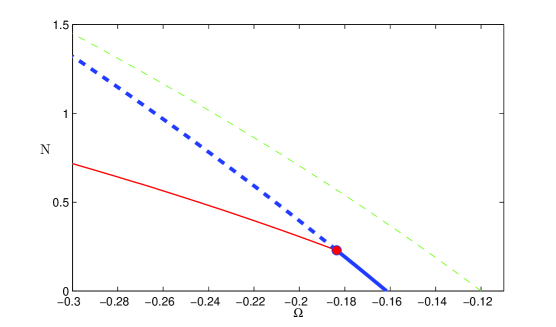
Figure 1: (Color Online) Bifurcation diagram for NLS-GP with double well potential (6.1) with parameters $s=1,L=6$ and cubic nonlinearity. The first bifurcation is from the the zero state at the ground state energy of the double well. Secondary bifurcation to an asymmetric state at ${\cal N}={\cal N}_{cr}$ is marked by a (red) circle. For ${\cal N}<{\cal N}_{cr}$ the symmetric state (thick (blue) solid line) is nonlinearly dynamically stable. For ${\cal N}>{\cal N}_{cr}$ the symmetric state is unstable (thick (blue) dashed line). The stable asymmetric state, appearing for ${\cal N}>{\cal N}_{cr}$, is marked by a thin (red) solid line. The (unstable) antisymmetric state is marked by a thin (green) dashed line.

The main results are stated in Theorem 4.1, Corollary 4.1 and Theorem 5.1. In particular, we obtain an asymptotic formula for the critical particle number (optical power) for symmetry breaking in NLS-GP,

$${\cal N}_{cr}\ =\ \frac{\Omega_{1}-\Omega_{0}}{\Xi[\psi_{0},\psi_{1}]}\ +\ {\cal O}\left(\ \frac{(\Omega_{1}-\Omega_{0})^{2}}{\Xi[\psi_{0},\psi_{1}]^{3}}\right).$$ (1.1)

Here, $(\Omega_{0},\psi_{0})$ and $(\Omega_{1},\psi_{1})$ are eigenvalue - eigenfunction pairs of the linear Schrödinger operator $H=-\Delta+V$, where $\Omega_{0}$ and $\Omega_{1}$ are separated from other spectrum, and $\Xi$ is a positive constant, given by (4.1), depending on $\psi_{0}$ and $\psi_{1}$. The most important case is where $\Omega_{0}<\Omega_{1}$ are the lowest two energies (linear ground and first excited states). For double wells with separation $L$, we have ${\cal N}_{cr}={\cal N}_{cr}(L)$, depending on the eigenvalue spacing $\Omega_{0}(L)-\Omega_{1}(L)$, which is exponentially small if $L$ is large and $\Xi$ is of order one. Thus, for large $L$, the bifurcation occurs at small $L^{2}$ norm. This is the weakly nonlinear regime in which the corrections to the finite dimensional model can be controlled perturbatively. A local bifurcation diagram of this type will occur for any simple even-odd symmetric pair of simple eigenvalues of $H$ in the weakly nonlinear regime, so long as the eigen-frequencies are separated from the rest of the spectrum of $H$; see Proposition 4.1 and the Gap Condition (4.7). Therefore, a similar phenomenon occurs for higher order, nearly degenerate pairs of eigen-states of the double wells, arising from isolated single wells with multiple eigenstates. Section 6 contains numerical results validating our theoretical analysis.

Acknowledgements: The authors acknowledge the support of the US National Science Foundation, Division of Mathematical Sciences (DMS). EK was partially supported by grants DMS-0405921 and DMS-060372. PGK was supported, in part, by DMS-0204585, NSF-CAREER and DMS-0505663, and acknowledges valuable discussions with T. Kapitula and Z. Chen. MIW was supported, in part, by DMS-0412305 and DMS-0530853. Part of this research was done while Eli Shlizerman was a visiting graduate student in the Department of Applied Physics and Applied Mathematics at Columbia University.

2 Technical formulation

Consider the initial-value-problem for the time-dependent nonlinear Schrödinger / Gross-Pitaevskii equation (NLS-GP)

$$i\partial_{t}\psi\ =\ H\psi\ +\ g(x)K[\ \psi\bar{\psi}\ ]\ \psi,\ \ \ \psi(x,0)\ {\rm given}$$ (2.1)

$$H\ =\ -\Delta+V(x).$$ (2.2)

We assume:

• The initial value problem for NLS-GP is well-posed in the space $C^{0}([0,\infty);H^{1}({\rm\hbox to0.0pt{I\hss}\,\bf R}^{n}))$.

(H2) The potential, $V(x)$ is assumed to be real-valued , smooth and rapidly decaying as $|x|\to\infty$. The basic example of $V(x)$, we have in mind is a double-well potential, consisting of two identical potential wells, separated by a distance $L$. Thus, we also assume symmetry with respect to the hyperplane, which without loss of generality can be taken to be $\{x_{1}=0\}$:

$$V(x_{1},x_{2},\dots,x_{n})\ =\ V(-x_{1},x_{2},\dots,x_{n}).$$ (2.3)

We assume the nonlinear term, $K[\psi\overline{\psi}]$, to be attractive, cubic ( local or nonlocal), and symmetric in one variable. Specifically, we assume the following
(H3) Hypotheses on the nonlinear term:

• $g(x_{1},x_{2},\ldots,x_{n})=g(-x_{1},x_{2},\ldots,x_{n})$ (symmetry)

• $g(x)<0$ (attractive / focusing)

• $K[h]=\int K(x-y)h(y)dy,\ \ \ K(x_{1},x_{2},\ldots,x_{n})=K(-x_{1},x_{2},\ldots,x_{n}),\ \ \ K>0$.

• Consider the map $N:H^{2}\times H^{2}\times H^{2}\mapsto L^{2}$ defined by

  $$N(\phi_{1},\phi_{2},\phi_{3})=gK[\phi_{1}\phi_{2}]\phi_{3}.$$ (2.4)

  We also write $N(u)=N(u,u,u)$ and note that $\partial_{u}N(u)=N(\cdot,u,u)+N(u,\cdot,u)+N(u,u,\cdot)$. We assume there exists a constant $k>0$ such that

  $$\|N(\phi_{0},\phi_{1},\phi_{2})\|_{L^{2}}\ \leq\ k\ \|\phi_{1}\|_{H^{2}}\|\phi_{2}\|_{H^{2}}\|\phi_{3}\|_{H^{2}}.$$ (2.5)

Several illustrative and important examples are now given:

Example 1: Gross-Pitaevskii equation for BECs with negative scattering
length $g(x)\equiv-1$, $K(x)=\delta(x)$
Example 2: Nonlinear Schrödinger equation for optical media with a nonlocal kernel $g(x)\equiv\pm 1$, $K(x)=A\exp(-x^{2}/\sigma^{2})$ [17] (see also [4] for similar considerations in BECs).
Example 3: Photorefractive nonlinearities The approach of the current paper can be adapted to the setting of photorefractive crystals with saturable nonlinearities and appropriate optically induced potentials [5]. The relevant symmetry breaking phenomenology is experimentally observable, as shown in [16].

Nonlinear bound states: Nonlinear bound states are solutions of NLS-GP of the form

$$\psi(x,t)\ =\ e^{-i\Omega t}\Psi_{\Omega}(x),$$ (2.6)

where $\Psi_{\Omega}\in H^{1}({\rm\hbox to0.0pt{I\hss}\,\bf R}^{n})$ solves

$$H\ \Psi_{\Omega}\ +\ g(x)\ K[|\Psi_{\Omega}|^{2}]\ \Psi_{\Omega}\ -\ {\Omega}\Psi_{\Omega}\ =\ 0,\ \ u\in H^{1}$$ (2.7)

If the potential $V(x)$ is such that the operator $H=-\Delta+V(x)$ has a discrete eigenvalue, $E_{*}$, and correspsonding eigenstate $\psi_{*}$, then for energies near $E$ near $E_{*}$ and one expects small amplitude nonlinear bound states, which are to leading order small multiples of $\psi_{*}$. This is the standard setting of bifurcation from a simple eigenvalue [19], which follows from the implicit function theorem.

Theorem 2.1

[20, 21] Let $(\Psi,E)=(\psi_{*},E_{*})$ be a simple eigenpair, of the eigenvalue problem $H\Psi={\Omega}\Psi$, i.e. $dim\{\rho:(H-E_{*})\rho=0\}=1$. Then, there exists a unique smooth curve of nontrivial solutions $\alpha\mapsto(\ \Psi(\cdot;\alpha),{\Omega}(\alpha)\ )$, defined in a neighborhood of $\alpha=0$, such that

$$\Psi_{\Omega}\ =\ \alpha\left(\ \psi_{0}\ +\ {\cal O}(|\alpha|^{2})\ \right),\ \ \Omega\ =\ \Omega_{0}\ +\ {\cal O}(|\alpha|^{2}),\ \ \alpha\to 0.$$ (2.8)

Remark 2.1

For a large class of problems, a nonlinear ground state can be characterized variationally as a constrained minimum of the NLS / GP energy subject to fixed squared $L^{2}$ norm. Define the NLS-GP Hamiltonian energy functional

$${\cal H}_{NLS-GP}[\Phi]\ \equiv\ \int|\nabla\Phi|^{2}\ +\ V|\Phi|^{2}\ dy\ +\ {1\over 2}\ \int\ g(y){\cal K}[|\Phi|^{2}]\ dy$$ (2.9)

and the particle number (optical power)

$${\cal N}[\Phi]\ =\ \int\ |\Phi|^{2}\ dy,$$ (2.10)

where

$${\cal K}[|\Phi|^{2}]\ =\ \int\ K(x-y)\ |\Phi(x)|^{2}\ |\Phi(y)|^{2}\ dy.$$ (2.11)

In particular, the following can be proved:

Theorem 2.2

Let $I_{\lambda}\ =\ \inf_{{\cal N}[f]=\lambda}\ {\cal H}[f]$. If $-\infty<I_{\lambda}<0$, then the minimum is attained at a positive solution of (2.7). Here, $\Omega=\Omega(\lambda)$ is a Lagrange multiplier for the constrained variational problem.

In [2] the nonlinear Hartree equation is studied; ${\cal K}[h]=|y|^{-1}\star h$, $g\equiv-1$. It is proved that if $V(x)$ is a double-well potential, then for $\lambda$ sufficiently large, the minimizer does not have the same symmetry as the linear ground state. By uniqueness, ensured by the implicit function theorem, for small ${\cal N}$, the minimizer has the same symmetry as that as the linear ground state and has the expansion (2.8); see [2] and section 4.

We make the following

Spectral assumptions on $H$

• $H$ has a pair of simple eigenvalues $\Omega_{0}$ and $\Omega_{1}$. $\psi_{0}$ and $\psi_{1}$, the corresponding (real-valued) eigenfunctions are, respectively, even and odd in $x_{1}.$

Example 2.1

The basic example: Double well potentials

A class of examples of great interest is that of double well potentials. The simplest example, in one space dimension, is obtained as follows; see section 8 for the multidimensional case. Start with a single potential well (rapidly decaying as $|x|\to\infty$), $v_{0}(x)$, having exactly one eigenvalue, $\omega$, $H_{0}\psi_{\omega}=(-\Delta+v_{0}(x))\psi_{\omega}=\omega\psi_{\omega}$; see Figure (2a). Center this well at $x=-L$ and place an identical well, centered at $x=L$. Denote by $V_{L}(x)$ the resulting double-well potential and $H_{L}$ denote the Schrödinger operator:

$$H_{L}=-\Delta+V_{L}(x)$$ (2.12)

There exists $L>L_{0}$, such that for $L>L_{0}$, $H_{L}$ has a pair of eigenvalues, $\Omega_{0}=\Omega_{0}(L)$ and $\Omega_{1}=\Omega_{1}(L)$, $\Omega_{0}<\Omega_{1}$, and corresponding eigenfunctions $\psi_{0}$ and $\psi_{1}$; see Figure (2b). $\psi_{0}$ is symmetric with respect to $x=0$ and $\psi_{1}$ is antisymmetric with respect to $x=0$. Moreover, for $L$ sufficiently large, $|\Omega_{0}-\Omega_{1}|={\cal O}(e^{-\kappa L}),\ \kappa>0$; see [8]; see also section 8.

(a)	(b)

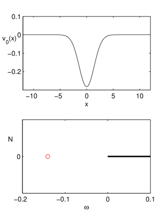
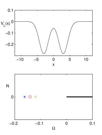
Figure 2: This figure demonstrates a single and a double well potential and the spectrum of $H$ and $H_{L}$ respectively. Panel (a) shows a single well potential and under it the spectrum of $H$, with an eigenvalue marked by a (red) mark ‘o’ at $\omega$ and continuous spectrum marked by a (black) line for energies $\omega\geq 0$. Panel (b) shows the double well centered at $\pm L$ and the spectrum of $H_{L}$ underneath. The eigenvalues $\Omega_{0}$ and $\Omega_{1}$ are each marked by a (blue) mark ‘*’ and a (green) mark ‘x’ respectively on either side of the location $\omega$ - (red) mark ‘o’. The continuous spectrum is marked by a (black) line for energies $\Omega\geq 0$.

The construction can be generalized. If $-\Delta+v_{0}(x)$ has $m$ bound states, then forming a double well $V_{L}$, with $L$ sufficiently large, $H_{L}=-\Delta+V_{L}$ will have $m-$ pairs of eigenvalues: $(\Omega_{2j},\Omega_{2j+1}),\ \ j=0,\dots,m-1$, eigenfunctions $\psi_{2j}$ (symmetric) and $\psi_{2j+1}$ anti-symmetric.

By Theorem 2.1, for small ${\cal N}$, there exists a unique non-trivial nonlinear bound state, bifurcating from the zero solution at the ground state energy, $\Omega_{0}$, of $H$. By uniqueness, ensured by the implicit function theorem, these small amplitude nonlinear bound states have the same symmetries as the double well; they are bi-modal. We also know from [2] that for sufficiently large ${\cal N}$ the ground state has broken symmetry. We now seek to elucidate the transition from the regime of ${\cal N}$ small to ${\cal N}$ large.

We work in the general setting of hypotheses (H1)-(H4). Define spectral projections onto the bound and continuous spectral parts of $H$:

$${P_{0}}=\left({\psi_{0}},\cdot\right){\psi_{0}},\ {P_{1}}=\left({\psi_{1}},\cdot\right){\psi_{1}},\ \ {\tilde{P}}=I\ -\ {P_{0}}\ -\ {P_{1}}$$ (2.13)

Here,

$$\left(f,g\right)\ =\ \int\ \bar{f}g\ dx.$$ (2.14)

We decompose the solutions of Eq. (2.7) according to

$$\Psi_{\Omega}\ =\ c_{0}{\psi_{0}}\ +\ c_{1}{\psi_{1}}\ +\ \eta,\ \ \eta={\tilde{P}}\eta.$$ (2.15)

We next substitute the expression (2.15) into equation (2.7) and then act with projections ${P_{0}}$, ${P_{1}}$ and ${\tilde{P}}$ to the resulting equation. Using the symmetry and anti-symmetry properties of the eigenstates, we obtain three equations which are equivalent to the PDE (2.7):

$$\left(\Omega_{0}-\Omega\right)c_{0}+a_{0000}|c_{0}|^{2}c_{0}+\left(a_{0110}+a_{0011}\right)|c_{1}|^{2}c_{0}+a_{0011}c_{1}^{2}\bar{c}_{0}+\left({\psi_{0}}g,{\cal R}(c_{0},c_{1},\eta)\right)\ =\ 0$$ (2.16)

$$\left(\Omega_{1}-\Omega\right)c_{1}+a_{1111}|c_{1}|^{2}c_{1}+\left(a_{1010}+a_{1001}\right)|c_{0}|^{2}c_{1}+a_{1010}c_{0}^{2}\bar{c}_{1}+\left({\psi_{1}}g,{\cal R}(c_{0},c_{1},\eta)\right)\ =\ 0$$ (2.17)

$$\left(H-{\Omega}\right)\ \eta\ =\ -{\tilde{P}}\ g\left[\ F(\cdot;c_{0},c_{1})\ +\ {\cal R}(c_{0},c_{1},\eta)\ \right]$$ (2.18)

$F(\cdot,c_{0},c_{1})$ is independent of $\eta$ and ${\cal R}(c_{0},c_{1},\eta)$ contains linear, quadratic and cubic terms in $\eta$. The coefficients $a_{klmn}$ are defined by:

$$a_{klmn}\ =\ \left(\ \psi_{k},gK[\psi_{l}\psi_{m}]\psi_{n}\ \right)$$ (2.19)

We shall study the character of the set of solutions of the system (2.16), (2.17), (2.18) restricted to the level set

$$\int|\Psi_{\Omega}|^{2}dx\ =\ {\cal N}\ \ \iff\ \ |c_{0}|^{2}\ +\ |c_{1}|^{2}\ +\ \int|\eta|^{2}dx\ =\ {\cal N}$$ (2.20)

as ${\cal N}$ varies.

Let $\Omega_{0}$ and $\Omega_{1}$ denote the two lowest eigenvalues of $H_{L}$. We prove (Theorem 4.1, Corollary 4.1, Theorem 5.1):

• There exist two solution branches, parametrized by ${\cal N}$, which bifurcate from the zero solution at the eigenvalues, $\Omega_{0}$ and $\Omega_{1}$.

• Along the branch, $(\Omega,\Psi_{\Omega})$, emanating from the solution $(\Omega=\Omega_{0},\Psi=0)$ , there is a symmetry breaking bifurcation at ${\cal N}={\cal N}_{crit}>0$. In particular, let $u_{crit}$ denote the solution of (2.7) corresponding to the value ${\cal N}={\cal N}_{crit}$. Then, in a neighborhood $u_{crit}$, for ${\cal N}<{\cal N}_{crit}$ there is only one solution of (2.7), the symmetric ground state, while for ${\cal N}>{\cal N}_{crit}$ there are two solutions one symmetric and a second asymmetric.

• Exchange of stability at the bifurcation point: For ${\cal N}<{\cal N}_{crit}$ the symmetric state is dynamically stable, while for ${\cal N}>{\cal N}_{crit}$ the asymmetric state is stable and the symmetric state is exponentially unstable.

3 Bifurcations in a finite dimensional approximation

It is illustrative to consider the finite dimensional approximation to the system (2.16,2.17,2.18), obtained by neglecting the continuous spectral part, ${\tilde{P}}u$. Let’s first set $\eta=0$, and therefore ${\cal R}(c_{0},c_{1},0)=0$. Under this assumption of no coupling to the continuous spectral part of $H$, we obtain the finite dimensional system:

$$\left(\Omega_{0}-\Omega\right)c_{0}+a_{0000}|c_{0}|^{2}c_{0}+\left(a_{0110}+a_{0011}\right)|c_{1}|^{2}c_{0}+a_{0011}c_{1}^{2}\bar{c}_{0}=\ 0$$ (3.1)

$$\left(\Omega_{1}-\Omega\right)c_{1}+a_{1111}|c_{1}|^{2}c_{1}+\left(a_{1010}+a_{1001}\right)|c_{0}|^{2}c_{1}+a_{1010}c_{0}^{2}\bar{c}_{1}\ =\ 0$$ (3.2)

$$|c_{0}|^{2}\ +\ |c_{1}|^{2}\ =\ {\cal N}$$ (3.3)

Our strategy is to first analyze the bifurcation problem for this approximate finite-dimensional system of algebraic equations. We then treat the corrections, coming from coupling to the continuous spectral part of $H$, $\eta$, perturbatively.

For simplicity we take $c_{j}$ real: $c_{j}=\rho_{j}\in{\rm\hbox to0.0pt{I\hss}\,\bf R}$; see section 4. Then,

$$\rho_{0}\ \left[\ \Omega_{0}-\Omega\ +\ a_{0000}\rho_{0}^{2}\ +\ \left(a_{0110}+2a_{0011}\right)\rho_{1}^{2}\ \right]=\ 0$$ (3.4)

$$\rho_{1}\ \left[\ \Omega_{1}-\Omega\ +\ a_{1111}\rho_{1}^{2}\ +\ \left(a_{1001}+2a_{1010}\right)\rho_{0}^{2}\ \right]\ =\ 0$$ (3.5)

$$\rho_{0}^{2}\ +\ \rho_{1}^{2}\ -\ {\cal N}\ =\ 0.$$ (3.6)

Introduce the notation

$${\cal P}_{0}=\rho_{0}^{2},\ \ {\cal P}_{1}=\rho_{1}^{2}$$ (3.7)

Then,

$${\cal F}_{0}({\cal P}_{0},{\cal P}_{1},{\Omega};{\cal N})\ =\ {\cal P}_{0}\ \left[\ \Omega_{0}-\Omega\ +\ a_{0000}{\cal P}_{0}\ +\ \left(a_{0110}+2a_{0011}\right){\cal P}_{1}\ \right]=\ 0$$

$${\cal F}_{1}({\cal P}_{0},{\cal P}_{1}.{\Omega};{\cal N})\ =\ {\cal P}_{1}\ \left[\ \Omega_{1}-\Omega\ +\ a_{1111}{\cal P}_{1}\ +\ \left(a_{1001}+2a_{1010}\right){\cal P}_{0}\ \right]\ =\ 0$$

$${\cal F}_{{\cal N}}({\cal P}_{0},{\cal P}_{1},{\Omega};{\cal N})\ ={\cal P}_{0}\ +\ {\cal P}_{1}\ -\ {\cal N}\ =\ 0.$$ (3.8)

Solutions of the approximate system

• ${\cal Q}^{(0)}({\cal N})\ =\ (\ {\cal P}_{0}^{(0)},{\cal P}_{1}^{(0)},{\Omega}^{(0)}\ )\ =\ (\ {\cal N},0,{\Omega_{0}}+a_{0000}{\cal N}\ )$ - approximate nonlinear ground state branch

• ${\cal Q}^{(1)}({\cal N})\ =\ (\ {\cal P}_{0}^{(1)},{\cal P}_{1}^{(1)},{\Omega}^{(1)}\ )\ =\ (\ 0,{\cal N},{\Omega_{1}}+a_{1111}{\cal N}\ )$ - approximate nonlinear excited state branch

Thus we have a system of equations ${\cal F}({\cal Q},{\cal N})=0$, where ${\cal F}:({\rm\hbox to0.0pt{I\hss}\,\bf R}_{+}\times{\rm\hbox to0.0pt{I\hss}\,\bf R}_{+}\times{\rm\hbox to0.0pt{I\hss}\,\bf R})\times{\rm\hbox to0.0pt{I\hss}\,\bf R}_{+}\to{\rm\hbox to0.0pt{I\hss}\,\bf R}^{3}\times{\rm\hbox to0.0pt{I\hss}\,\bf R}_{+}$, mapping $({\cal Q},{\cal N})\to{\cal F}({\cal Q},{\cal N})$ smoothly. We have that ${\cal F}({\cal Q}^{(j)}({\cal N}),{\cal N})=0,\ j=0,1$ for all ${\cal N}\geq 0$. A bifurcation (onset of multiple solutions) can occur only at a value of ${\cal N}_{*}$ for which the Jacobian $d_{\cal Q}{\cal F}({\cal Q}^{(j)}({\cal N}_{*});{\cal N}_{*})$ is singular. The point $({\cal Q}^{(j)}({\cal N}_{*});{\cal N}_{*})$ is called a bifurcation point. In a neighborhood of a bifurcation point there is a multiplicity of solutions (non-uniqueness) for a given ${\cal N}$. The detailed character of the bifurcation is suggested by the nature of the null space of $d_{\cal Q}{\cal F}({\cal Q}^{(j)}({\cal N}_{*});{\cal N}_{*})$.

We next compute $d_{\cal Q}{\cal F}({\cal Q}^{(j)}({\cal N});{\cal N})$ along the different branches in order to see whether and where there are bifurcations.

The Jacobian is given by

$$d_{\cal Q}{\cal F}({\cal Q}^{(j)}({\cal N});{\cal N})\ =\ \frac{\partial({\cal F}_{0},{\cal F}_{1},{\cal F}_{\cal N})}{\partial({\cal P}_{0},{\cal P}_{1},{\Omega})}\ =$$

$$\begin{pmatrix}{\Omega_{0}}-{\Omega}+2a_{0000}{\cal P}_{0}+(a_{0110}+a_{0011}){\cal P}_{1}&(a_{0110}+2a_{0011}){\cal P}_{0}&-P_{0}\\ (a_{1001}+2a_{1010}){\cal P}_{1}&{\Omega_{1}}-{\Omega}+2a_{1111}{\cal P}_{1}+(a_{0110}+2a_{1010}){\cal P}_{0}&-{\cal P}_{1}\\ 1&1&0\end{pmatrix}$$ (3.9)

A candidate value of ${\cal N}$ for which there is a bifurcation point along the “ground state branch” is one for which

$$\det\left(\ d_{\cal Q}{\cal F}({\cal Q}^{(0)}({\cal N});{\cal N})\ \right)\ =\ 0\ \ \iff\ \ {\cal N}\ =\ {{\cal N}_{cr}^{(0)}}\ \equiv\ \frac{{\Omega_{1}}-{\Omega_{0}}}{a_{0000}-(a_{1001}+2a_{1010})}$$ (3.10)

Since the parameter ${\cal N}$ is positive, we have

Proposition 3.1

• ${\cal Q}^{(0)}({{\cal N}_{cr}^{(0)}})\ =\ ({{\cal N}_{cr}^{(0)}},0,{\Omega_{0}}+a_{0000}{{\cal N}_{cr}^{(0)}};{{\cal N}_{cr}^{(0)}})$ is a bifurcation point for the approximating system (3.4-3.6) if ${{\cal N}_{cr}^{(0)}}$ is positive.

• For the double well with well-separation parameter, $L$, we have that ${{\cal N}_{cr}^{(0)}}(L)>0$ for $L$ sufficiently large.

Proof: We need only check (b). This is easy to see, using the large $L$ approximations of $\psi_{0}$ and $\psi_{1}$ in terms of $\psi_{\omega}$, the ground state of $H=-\Delta+V(x)$, the “single well” operator:

$${\psi_{0}}\ \sim\ 2^{-1/2}\left(\ \psi_{\omega}(x-L)+\psi_{\omega}(x+L)\ \right)$$

$${\psi_{1}}\ \sim\ 2^{-1/2}\left(\ \psi_{\omega}(x-L)-\psi_{\omega}(x+L)\ \right);$$ (3.11)

see Proposition 8.1 in section 8.

Excited state branch

$$\det\left(\ d_{\cal Q}{\cal F}({\cal Q}^{(1)}({\cal N});{\cal N})\ \right)\ =\ 0\ \iff\ \ {\cal N}_{*}^{(1)}\ =\ \frac{{\Omega_{1}}-{\Omega_{0}}}{a_{0110}+2a_{0011}-a_{1111}}$$ (3.12)

Remark 3.1

For the double well with well-separation parameter, $L$, we have that ${\cal N}^{(1)}_{*}(L)~{}<~{}0$ for $L$ sufficiently large, as can be checked using the approximation (3.11). Therefore ${\cal Q}^{(1)}({\cal N}_{*}^{(1)})$ is not a bifurcation point of the approximating system (3.8).

Summary: Assume ${\cal N}$ is sufficiently small. The finite dimensional approximation (3.8) predicts a symmetry breaking bifurcation along the nonlinear ground state branch and that no bifurcation takes place along the anti-symmetric branch of nonlinear bound states.

4 Bifurcation / Symmetry breaking analysis of the PDE

In this section we prove the following

Theorem 4.1

(Symmetry Breaking for NLS-GP) Consider NLS-GP with hypotheses (H2)-(H4). Let $a_{klmn}$ be given by (2.19) and

$$\Xi[\psi_{0},\psi_{1},g]\ \equiv a_{0000}-a_{1001}-2a_{1010}$$

$$=\left(\psi_{0}^{2},gK[\psi_{0}^{2}]\right)-\left(\psi_{1}^{2},gK[\psi_{0}^{2}]\right)-2\left(\psi_{0}\psi_{1},gK[\psi_{0}\psi_{1}]\right)\ >\ 0.$$ (4.1)

Assume

$$\frac{\Omega_{1}-\Omega_{0}}{\Xi[\psi_{0},\psi_{1}]^{2}}\ \ {\rm is\ sufficiently\ small.}$$ (4.2)

Then, there exists ${\cal N}_{cr}>0$ such that

• for any ${\cal N}\leq{\cal N}_{cr}$, there is (up to the symmetry $u\mapsto u\ e^{i\gamma}$) a unique ground state, $u_{\cal N}$, having the same spatial symmetries as the double well.

• ${\cal N}={\cal N}_{cr},\ u^{sym}_{{\cal N}_{cr}}$ is a bifurcation point. For ${\cal N}>{\cal N}_{cr}$, there are, in a neighborhood of ${\cal N}={\cal N}_{cr},\ u^{sym}_{{\cal N}_{cr}}$, two branches of solutions: (a) a continuation of the symmetric branch, and (b) a new asymmetric branch.

• The critical ${\cal N}$- value for bifurcation is given approximately by

  $${\cal N}_{cr}\ \ =\ \frac{\Omega_{1}-\Omega_{0}}{\Xi[\psi_{0},\psi_{1}]}\left[1+{\cal O}\left(\ \frac{\Omega_{1}-\Omega_{0}}{\Xi[\psi_{0},\psi_{1}]^{2}}\right)\right]$$

Corollary 4.1

Fix a pair of eigenvalues, $(\Omega_{2j},\psi_{2j}),\ (\Omega_{2j+1},\psi_{2j+1})$ of the linear double-well potential, $V_{L}(x)$; see Example 2.1. For the NLS-GP with double well potential of well-separation $L$, there exists $\tilde{L}>0$, such that for all $L\geq\tilde{L}$, there is a symmetry breaking bifurcation, as described in Theorem 4.1, with ${\cal N}_{cr}={\cal N}_{cr}(L;j)$.

Remark 4.1

$\Omega_{1}(L)-\Omega_{0}(L)\ =\ {\cal O}(e^{-\kappa L})$ for $L$ large. The terms in $\Xi[\psi_{0},\psi_{1}](L)$ are ${\cal O}(1)$. Therefore, for the double well potential, $V_{L}(x)$, the smallness hypothesis of Theorem 4.1 holds provided $L$ is sufficiently large.

To prove this theorem we will establish that, under hypotheses (4.1)-(4.2), the character of the solution set (symmetry breaking bifurcation) of the finite dimensional approximation (3.1-3.3) persists for the full (infinite dimensional) problem:

$$\left(\Omega_{0}-\Omega\right)c_{0}+a_{0000}|c_{0}|^{2}c_{0}+\left(a_{0110}+a_{0011}\right)|c_{1}|^{2}c_{0}+a_{0011}c_{1}^{2}\bar{c}_{0}+\left({\psi_{0}}g,{\cal R}(c_{0},c_{1},\eta)\right)\ =\ 0$$ (4.3)

$$\left(\Omega_{1}-\Omega\right)c_{1}+a_{1111}|c_{1}|^{2}c_{1}+\left(a_{1010}+a_{1001}\right)|c_{0}|^{2}c_{1}+a_{1010}c_{0}^{2}\bar{c}_{1}+\left({\psi_{1}}g,{\cal R}(c_{0},c_{1},\eta)\right)\ =\ 0$$ (4.4)

$$\left(H-{\Omega}\right)\ \eta\ =\ -{\tilde{P}}\ g\left[\ F(\cdot;c_{0},c_{1})\ +\ {\cal R}(c_{0},c_{1},\eta)\ \right],\ \ \ \ \ \eta={\tilde{P}}\eta$$ (4.5)

$$|c_{0}|^{2}\ +\ |c_{1}|^{2}\ +\ \int|\eta|^{2}\ \ =\ {\cal N}.$$ (4.6)

We analyze this system using the Lyapunov-Schmidt method. The strategy is to solve equation (4.5) for $\eta$ as a functional of $c_{0},c_{1}$ and $\Omega$. Then, substituting $\eta=\eta[c_{0},c_{1},\Omega]$ into equations (4.3), (4.4) and (4.6), we obtain three closed equations, depending on a parameter ${\cal N}$, for $c_{0},c_{1}$ and $\Omega$. This system is a perturbation of the finite dimensional (truncated) system: (3.1, 3.2) and (3.3). We then show that under hypotheses (4.1)-(4.2) there is a symmetry breaking bifurcation. Finally, we show that the terms perturbing the finite dimensional model have a small and controllable effect on the character of the solution set for a range of ${\cal N}$, which includes the bifurcation point. Note that, in the double well problem, hypotheses (4.1)-(4.2) are satisfied for $L$ sufficiently large, see Proposition 8.2.

We begin with the following proposition, which characterizes $\eta=\eta[c_{0},c_{1},\Omega]$.

Proposition 4.1

Consider equation (4.5) for $\eta$. By (H4) we have the following:

$${\rm Gap\ Condition:}\ |\Omega_{j}-\tau|\ \geq\ 2d_{*}\ {\rm for}\ j=0,1\ {\rm and\ all}\ \ \tau\in\sigma(H)\setminus\{\Omega_{0},\Omega_{1}\}$$ (4.7)

Then there exists $n_{*},\ r_{*}>0$, depending on $d_{*}$, such that in the open set

$$|c_{0}|+|c_{1}| < r_{*}$$ (4.8)

$$\|c_{0}{\psi_{0}}+c_{1}{\psi_{1}}+\eta\|_{H^{2}} < n_{*}(d_{*})$$

$$dist(\Omega,\sigma(H)\setminus\{\Omega_{0},\Omega_{1}\}) > d_{*},$$ (4.9)

the unique solution of (2.18) is given by the real-analytic mapping:

$$(c_{0},c_{1},\Omega)\ \mapsto\ \ \eta[c_{0},c_{1},\Omega],$$ (4.10)

defined on the domain given by (4.8,4.9). Moreover there exists $C_{*}>0$ such that:

$$\|\ \eta[c_{0},c_{1},\Omega]\ \|_{H^{2}}\leq C_{*}(|c_{0}|+|c_{1}|)^{3}$$ (4.11)

Proof: Consider the map

$$N:H^{2}\times H^{2}\times H^{2}\mapsto L^{2}$$

$$N(\phi_{0},\phi_{1},\phi_{2})=gK[\phi_{1}\phi_{2}]\phi_{3}.$$

By assumptions on the nonlinearity (see section 2), there exists a constant $k>0$ such that

$$\|N(\phi_{0},\phi_{1},\phi_{2})\|_{L^{2}}\leq k\|\phi_{1}\|_{H^{2}}\|\phi_{2}\|_{H^{2}}\|\phi_{3}\|_{H^{2}}.$$ (4.12)

Moreover the map being linear in each component it is real analytic.

Let $c_{0},c_{1}$ and $\Omega$ be restricted according the inequalities (4.8,4.9). Equation (2.18) can be rewritten in the form

$$\eta+(H-\Omega)^{-1}{\tilde{P}}N[c_{0}{\psi_{0}}+c_{1}{\psi_{1}}+\eta]\ =\ 0.$$ (4.13)

Since the spectrum of $H{\tilde{P}}$ is bounded away from $\Omega$ by $d_{*}$, the resolvent:

$$(H-\Omega)^{-1}{\tilde{P}}:L^{2}\mapsto H^{2}$$

is a (complex) analytic map and bounded uniformly,

$$\|(H-\Omega)^{-1}{\tilde{P}}\|_{L^{2}\mapsto H^{2}}\leq p(d_{*}^{-1}),$$ (4.14)

where $p(s)\to\infty$ as $s\to\infty$. Consequently the map $F:\mathbb{C}^{2}\times\{\Omega\in\mathbb{C}\ :\ dist(\Omega,\sigma(H)\setminus\{\Omega_{0},\Omega_{1}\}\ \}\geq d_{*}\}\times H^{2}\mapsto H^{2}$ given by

$$F(c_{0},c_{1},\Omega,\eta)=\eta+(H-\Omega)^{-1}{\tilde{P}}N[\ c_{0}{\psi_{0}}+c_{1}{\psi_{1}}+\eta\ ]$$ (4.15)

is real analytic. Moreover,

$$F(0,0,\Omega,0)=0,\ \ \ D_{\eta}F(0,0,\Omega,0)=I.$$

Applying the implicit function theorem to equation (4.13), we have that there exists $n_{*}(\Omega),\ r_{*}(\Omega)$ such that whenever $|c_{0}|+|c_{1}|<r_{*}$ and $\|c_{0}{\psi_{0}}+c_{1}{\psi_{1}}+\eta\|_{H^{2}}<n_{*}$ equation (4.13) has an unique solution:

$$\eta=\eta(c_{0},c_{1},\Omega)\in H^{2}$$

which depends analytically on the parameters $c_{0},\ c_{1},\ \Omega.$ By applying the projection operator ${\tilde{P}}$ to the (4.13) which commutes with $(H-\Omega)^{-1}$ we immediately obtain ${\tilde{P}}\eta=\eta,$ i.e. $\eta\in{\tilde{P}}L^{2}.$

We now show that $n_{*},\ r_{*}$ can be chosen independent of $\Omega$, satisfying (4.9). The implicit function theorem can be applied in an open set for which

$$D_{\eta}F(c_{0},c_{1},\Omega,\eta)=I+(H-\Omega)^{-1}{\tilde{P}}D_{\eta}N[\ c_{0}{\psi_{0}}+c_{1}{\psi_{1}}+\eta\ ]$$

is invertible. For this it suffices to have:

$$\|\ (H-\Omega)^{-1}{\tilde{P}}D_{\eta}N[\ c_{0}{\psi_{0}}+c_{1}{\psi_{1}}+\eta]\ \|_{H^{2}}\leq Lip<1$$

A direct application of (4.12) and (4.14) shows that

$$\|(H-\Omega)^{-1}{\tilde{P}}D_{\eta}N[\ c_{0}{\psi_{0}}+c_{1}{\psi_{1}}+\eta]\ \|_{H^{2}}\leq$$

$$3k\ p(d_{*}^{-1})\ \|c_{0}{\psi_{0}}+c_{1}{\psi_{1}}+\eta\|_{H^{2}}^{2}$$ (4.16)

Fix $Lip=3/4.$ Then, a sufficient condition for invertibility is

$$3k\ p(d_{*}^{-1})\ \|c_{0}{\psi_{0}}+c_{1}{\psi_{1}}+\eta\|_{H^{2}}^{2}\leq Lip=3/4.$$ (4.17)

which allows us to choose $n_{*}=\frac{1}{2}\sqrt{\frac{1}{kp(d_{*}^{-1})}}$, independently of $\Omega.$

But, if (4.17) holds, then, from (4.16), the $H^{2}$ operator

$$(H-\Omega)^{-1}{\tilde{P}}N[\ c_{0}{\psi_{0}}+c_{1}{\psi_{1}}+\cdot\ ]$$

is Lipschitz with Lipschitz constant less or equal to $Lip=3/4.$ The standard contraction principle estimate applied to (4.13) gives:

$$\|\eta\|_{H^{2}} \leq \frac{1}{1-Lip}\|(H-\Omega)^{-1}{\tilde{P}}N[\ c_{0}{\psi_{0}}+c_{1}{\psi_{1}}\ ]\ \|_{H^{2}}$$ (4.18)

$$\leq 4p(d_{*}^{-1})\ k\|c_{0}{\psi_{0}}+c_{1}{\psi_{1}}\|_{H^{2}}^{3}.$$

Plugging the above estimate into (4.17) gives:

$$\|c_{0}{\psi_{0}}+c_{1}{\psi_{1}}\|_{H^{2}}+4p(d_{*}^{-1})\ k\|c_{0}{\psi_{0}}+c_{1}{\psi_{1}}\|_{H^{2}}^{3}\leq\frac{1}{2\sqrt{p(d_{*}^{-1})k}}$$

Since the left hand side is continuous in $(c_{0},c_{1})\in\mathbb{C}^{2}$ and zero for $c_{0}=c_{1}=0$ one can construct $r_{*}>0$ depending only on $d_{*},\ k$ such that the above inequality, hence (4.17) and (4.18), all hold whenever $|c_{0}|+|c_{1}|\leq r_{*}.$ Finally, (4.11) now follows from (4.18).QED

In particular, for the double well potential we have the following

Proposition 4.2

Let $V=V_{L}$ denote the double well potential with well-separation $L$. There exists $L_{*}>0,\ \varepsilon(L_{*})>0$ and $d_{*}(L_{*})>0$ such that for $L>L_{*},$ we have that for $(c_{0},c_{1},\Omega)$ satisfying $dist(\Omega,\sigma(H)\setminus\{\Omega_{0},\Omega_{1}\}\}\ \}\geq d_{*}(L_{*})$ and $|c_{0}|+|c_{1}|<\varepsilon(L_{*})$ $\eta[c_{0},c_{1},\Omega]$ is defined and analytic and satisfies the bound (4.11) for some $C_{*}>0$.

Proof: Since $\Omega_{0},\ \Omega_{1},\ {\psi_{0}}$ and ${\psi_{1}}$ can be controlled, uniformly in $L$ large, via the approximations (3.11), both $d_{*}$ and $r_{*}$ in the previous Proposition can be controlled uniformly in $L$ large. QED

Next we study the symmetries of $\eta(c_{0},c_{1},\Omega)$ and properties of ${\cal R}(c_{0},c_{1},\eta)$ which we will use in analyzing the equations (2.16)-(2.17). The following result is a direct consequence of the symmetries of equation (2.18) and Proposition 4.1:

Proposition 4.3

We have

$$\eta(e^{i\theta}c_{0},e^{i\theta}c_{1},\Omega)=e^{i\theta}\eta(c_{0},c_{1},\Omega),\qquad{\rm for}\ 0\leq\theta<2\pi,$$ (4.19)

$$\overline{\eta(c_{0},c_{1},\Omega)}=\eta(\overline{c_{0}},\overline{c_{1}},\overline{\Omega})$$ (4.20)

in particular

$$\eta(e^{i\theta}c_{0},c_{1}=0,\Omega)=e^{i\theta}\eta(c_{0},c_{1}=0,\Omega),$$ (4.21)

$$\eta(c_{0}=0,e^{i\theta}c_{1},\Omega)=e^{i\theta}\eta(c_{0}=0,c_{1},\Omega),$$ (4.22)

$\eta(c_{0},0,\Omega)$ is even in $x_{1},$ $\eta(0,c_{1},\Omega)$ is odd in $x_{1}$ and if $c_{0},\ c_{1}$ and $\Omega$ are real valued, then $\eta(c_{0},c_{1},\Omega)$ is real valued.

In addition

$$\langle\ {\psi_{0}},{\cal R}(c_{0},c_{1},\eta)\ \rangle\ =\ c_{0}\ f_{0}\left(\ c_{0},c_{1},\Omega\ \right)$$ (4.23)

$$\langle\ {\psi_{1}},{\cal R}(c_{0},c_{1},\eta)\ \rangle\ =\ c_{1}\ f_{1}\left(\ c_{0},c_{1},\Omega\ \right)$$ (4.24)

where, for any $0\leq\theta<2\pi$

$$f_{j}\left(e^{i\theta}c_{0},e^{i\theta}c_{1},\Omega\ \right)=f_{j}\left(\ c_{0},c_{1},\Omega\ \right),\qquad j=0,1$$ (4.25)

$$\overline{f_{j}(c_{0},c_{1},\Omega\ )}=f_{j}\left(\ \overline{c_{0}},\overline{c_{1}},\overline{\Omega}\ \right),\qquad j=0,1$$ (4.26)

$$\left|f_{j}\left(\ c_{0},c_{1},\Omega\ \right)\right|\leq C(|c_{0}|+|c_{1}|)^{4},\qquad j=0,1$$ (4.27)

for some constant $C>0.$ Moreover, both $f_{0}$ and $f_{1}$ can be written as absolutely convergent power series:

$$f_{j}(c_{0},c_{1},\Omega)=\sum_{k+l+m+n\geq 4,\ k-l+m-n=0,\ m+n={\rm even}}b^{j}_{klmn}(\Omega)c_{0}^{k}\ \overline{c}_{0}^{l}\ c_{1}^{m}\ \overline{c}_{1}^{n},\qquad j=0,1,$$ (4.28)

where $b^{j}_{klmn}(\Omega)$ are real valued when $\Omega$ is real valued. In particular, if $c_{0},\ c_{1}$ and $\Omega$ are real valued, then $f_{j}\left(c_{0},c_{1},\Omega\ \right)$ is real valued and, in polar coordinates, for $c_{0},c_{1}\not=0,$ we have

$$f_{j}(|c_{0}|,|c_{1}|,{\Delta\theta},\Omega)=\sum_{k+m\geq 2,\ p\in\mathbb{Z}}b^{j}_{kmp}(\Omega)e^{ip2{\Delta\theta}}|c_{0}|^{2k}|c_{1}|^{2m},\qquad j=0,1,$$ (4.29)

where ${\Delta\theta}$ is the phase difference between $c_{1}\in\mathbb{C}$ and $c_{0}\in\mathbb{C}.$

Proof of Proposition 4.3: We start with (4.19) which clearly implies (4.21)-(4.22). We fix $\Omega$ and suppress dependence on it in subsequent notation. From equation (4.13) we have:

$$\eta(e^{i\theta}c_{0},e^{i\theta}c_{1})$$

$$= -(H-\Omega)^{-1}{\tilde{P}}N(e^{i\theta}c_{0}{\psi_{0}}+e^{i\theta}c_{1}{\psi_{1}}+\eta,e^{i\theta}c_{0}{\psi_{0}}+e^{i\theta}c_{1}{\psi_{1}}+\eta,e^{i\theta}c_{0}{\psi_{0}}+e^{i\theta}c_{1}{\psi_{1}}+\eta)$$

$$= -(H-\Omega)^{-1}{\tilde{P}}e^{i\theta}N(c_{0}{\psi_{0}}+c_{1}{\psi_{1}}+e^{-i\theta}\eta,c_{0}{\psi_{0}}+c_{1}{\psi_{1}}+e^{-i\theta}\eta,c_{0}{\psi_{0}}+c_{1}{\psi_{1}}+e^{-i\theta}\eta)$$

where we used

$$N(a\phi_{1},b\phi_{2},c\phi_{3})=a\overline{b}cN(\phi_{1},\phi_{2},\phi_{3}).$$ (4.30)

Consequently

$$e^{-i\theta}\eta(e^{i\theta}c_{0},e^{i\theta}c_{1})=-(H-\Omega)^{-1}{\tilde{P}}N[\ c_{0}{\psi_{0}}+c_{1}{\psi_{1}}+e^{-i\theta}\eta,c_{0}{\psi_{0}}+c_{1}{\psi_{1}}+e^{-i\theta}\eta,c_{0}{\psi_{0}}+c_{1}{\psi_{1}}+e^{-i\theta}\eta]$$

which shows that both $e^{-i\theta}\eta(e^{i\theta}c_{0},e^{i\theta}c_{1})$ and $\eta(c_{0},c_{1})$ satisfy the same equation (4.13). From the uniqueness of the solution proved in Proposition 4.1 we have the relation (4.19).

A similar argument (and use of the complex conjugate) leads to (4.20) and to the parities of $\eta(c_{0},0)$ and $\eta(0,c_{1}).$

To prove (4.23) and (4.24), recall that

$${\cal R}\left(c_{0},c_{1},\eta(c_{0},c_{1},\Omega)\right) = N(c_{0}{\psi_{0}}+c_{1}{\psi_{1}}+\eta,c_{0}{\psi_{0}}+c_{1}{\psi_{1}}+\eta,c_{0}{\psi_{0}}+c_{1}{\psi_{1}}+\eta)$$ (4.31)

$$- N(c_{0}{\psi_{0}}+c_{1}{\psi_{1}},c_{0}{\psi_{0}}+c_{1}{\psi_{1}},c_{0}{\psi_{0}}+c_{1}{\psi_{1}}).$$

Consider first the case $c_{1}=\rho_{1}\in\mathbb{R}.$ Note that

$$\langle\ {\psi_{1}}g,{\cal R}(c_{0},\rho_{1}=0,\eta(c_{0},0))\ \rangle\ =\ 0.$$

Indeed, for $\rho_{1}=0,$ all the functions in the arguments of ${\cal R}$ are even functions (in $x_{1}$) making ${\cal R}$ an even function. Since ${\psi_{1}}$ is odd we get that the above is the integral over the entire space of an odd function, i.e. zero. Since $\langle\ {\psi_{1}},{\cal R}(c_{0},\rho_{1},\eta(c_{0},\rho_{1}))\ \rangle$ is analytic in $\rho_{1}\in\mathbb{R}$ by the composition rule, and its Taylor series starts with zero we get (4.24) for real $c_{1}=\rho_{1}.$ To extend the result for complex values $c_{1}$ we use the rotational symmetry of ${\cal R},$ namely from (4.19), (4.30) and (4.31) we have

$${\cal R}\left(e^{i\theta}c_{0},e^{i\theta}c_{1},\eta(e^{i\theta}c_{0},e^{i\theta}c_{1},\Omega)\right)=e^{i\theta}{\cal R}\left(c_{0},c_{1},\eta(c_{0},c_{1},\Omega)\right),\qquad 0\leq\theta<\pi$$

hence (4.24) holds for $c_{1}=|c_{1}|e^{-i\theta}$ by extending $f_{1}$ via the equality (4.25).

A very similar argument holds for (4.23). Equation (4.27) follows from the definition of ${\cal R}$ and (4.11). Equation (4.26) follows from (4.20).

We now turn to a proof of the expansions for $f_{j}$: (4.28) and (4.29). Note first that both $f_{0}$ and $f_{1}$ are real analytic in $c_{0},\ c_{1}$ by analyticity of ${\cal R}$ in (4.23)-(4.24); see (4.31). Note also that $\eta$ is real analytic by Proposition 4.1 while $N$ is trilinear. Hence, both $f_{0}$ and $f_{1}$ can be written in power series of the type (4.28). Estimate (4.27) implies that $k+l+m+n\geq 4,$ while the rotational invariance (4.25) implies $k-l+m-n=0.$ The following parity argument shows why $m+n$ hence $m-n=l-k$ and $k+l$ are all even. Assume $m+n$ is odd. Note that because of (4.23), $b^{0}_{klmn}$ is the scalar product between an even function (in $x_{1}$) ${\psi_{0}}$ and the term in the power series of ${\cal R}$ in which ${\psi_{1}}$ is repeated $m+n$ times. The latter is an odd function (in $x_{1}$) because ${\psi_{1}}$ is an odd function and it is repeated an odd number of times. The scalar product and hence $b^{0}_{klmn}$ for $m+n$ odd will be zero. A similar argument holds for $b^{1}_{klmn},\ m+n$ odd. Finally $b^{j}_{klmn}(\Omega)$ are real valued when $\Omega$ is real because they are scalar products of real valued functions.

The form (4.29) of the power series follows directly from (4.28) by expressing $c_{0}$ and $c_{1}$ in their polar forms: $c_{0}=|c_{0}|e^{i\theta_{0}}$ and $c_{1}=|c_{1}|e^{i\theta_{1}},\ {\Delta\theta}=\theta_{1}-\theta_{0}$, and using that $m+n,\ k+l$ and $m-n=-(k-l)$ are all even. The proof of Proposition 4.3 is now complete.

4.1 Ground state and excited state branches, pre-bifurcation

In this section we prove part (i) of Theorem 4.1 as well as a corresponding statement about the excited state. In particular, we show that for sufficiently small amplitude, the only nonlinear bound state families are those arising via bifurcation from the zero state at the eigenvalues $\Omega_{0}$ and $\Omega_{1}$. This is true for general potentials with two bound states. Here, however we can determine threshold amplitude, ${\cal N}_{cr}$, above which the solution set changes.

A closed system of equations for $c_{0},c_{1}$ and $\Omega$, parametrized by ${\cal N}$, is obtained upon substitution of $\eta[c_{0},c_{1},\Omega]$, (Proposition 4.1) into (4.3-4.6). Furthermore, using the structural properties (4.23-4.24) of Proposition 4.3, we obtain:

$$\left(\Omega_{0}-\Omega\right)c_{0}+a_{0000}|c_{0}|^{2}c_{0}+\left(a_{0110}+a_{0011}\right)|c_{1}|^{2}c_{0}+a_{0011}c_{1}^{2}\bar{c}_{0}+c_{0}f_{0}(c_{0},c_{1},\Omega)\ =\ 0$$ (4.32)

$$\left(\Omega_{1}-\Omega\right)c_{1}+a_{1111}|c_{1}|^{2}c_{1}+\left(a_{1010}+a_{1001}\right)|c_{0}|^{2}c_{1}+a_{1010}c_{0}^{2}\bar{c}_{1}+c_{1}f_{1}(c_{0},c_{1},\Omega)\ =\ 0$$ (4.33)

$$|c_{0}|^{2}\ +\ |c_{1}|^{2}\ +{\cal O}\left(|c_{0}|^{2}+|c_{1}|^{2}\right)^{3}\ =\ {\cal N}$$ (4.34)

This system of equations is valid for $|c_{0}|+|c_{1}|<r_{*}$, independent of $L$, the distance between wells.

If we choose $c_{1}=0$, then the second equation in the system (4.32) is satisfied. In this case, a non-trivial solution requires $c_{0}\neq 0$. The first equation, (4.33), after factoring out $c_{0}$ becomes

$$\Omega_{0}-\Omega+a_{0000}|c_{0}|^{2}+f_{0}(|c_{0}|,0,\Omega)\ =\ 0$$ (4.35)

where we used (4.25) to eliminate the phase of the complex quantity $c_{0}$. Since $\Omega$ is real (4.35) becomes one equation with two real parameters $\Omega,\ |c_{0}|.$ Since the right hand side of (4.35) vanishes for $\Omega=\Omega_{0}$ and $|c_{0}|=0$ and since the partial derivative of this function with respect to $\Omega$, evaluated at this solution, is non-zero, we have by the implicit function theorem that there is a unique solution

$$\Omega=\Omega_{g}(|c_{0}|)=\Omega_{0}+a_{0000}|c_{0}|^{2}+{\cal O}(|c_{0}|^{4}).$$ (4.36)

By (4.34), for small amplitudes, the mapping from $|c_{0}|^{2}+|c_{1}|^{2}$ to ${\cal N}$ is invertible. The family of solutions

$$|c_{0}|\ \mapsto\ \left(\ |c_{0}|e^{i\theta},|c_{1}|=0,\Omega=\Omega_{g}(|c_{0}|)\ \right),\ \ \theta_{0}\in[0,2\pi)$$

defined for $|c_{0}|$ sufficiently small, corresponds to a family of symmetric nonlinear bound states, $u_{\cal N}$ with $\|u_{\cal N}\|_{L^{2}}^{2}={\cal N}$, bifurcating from the zero solution at the linear eigenvalue $\Omega_{0}$

$$u_{\cal N}\ =\ \left(\ |c_{0}|{\psi_{0}}(x)\ +\ \eta[|c_{0}|,0,\Omega_{g}(|c_{0}|](x)\ \right)\ e^{i\theta_{0}},\ \ \theta_{0}\in[0,2\pi)$$

$$\Omega\ =\ \Omega_{g}(|c_{0}|);$$

see, for example, [20, 21]. Since both ${\psi_{0}}$ and $\eta(|c_{0}|,0,\Omega_{g})$ are even (in $x_{1}$) we infer that $u_{\cal N}$ is symmetric (even).

Remark 4.2

A similar result holds for the case $c_{0}=0$ leading to the anti-symmetric excited state branch.

Proposition 4.4

For $|c_{0}|+|c_{1}|$ sufficiently small, these two branches of solutions, are the only solutions non-trivial solutions of (2.7).

Proof:  Indeed, suppose the contrary. By local uniqueness of these branches, ensured by the implicit function theorem, a solution not already lying on one of these branches must have both $c_{0}$ and $c_{1}$ nonzero. Now, divide the first equation by $c_{0}$, the second equation by $c_{1},$ and subtract the results. Introducing polar coordinates:

$$c_{0}=\rho_{0}e^{i\theta_{0}},\ c_{1}=\rho_{1}e^{i\theta_{1}},\ {\Delta\theta}=\theta_{1}-\theta_{0},$$ (4.37)

we obtain:

$$\Omega_{1}-\Omega_{0} = a_{0000}\rho_{0}^{2}\ +\ \left(a_{0110}+a_{0011}+a_{0011}e^{i2{\Delta\theta}}\right)\rho_{1}^{2}\ +\ f_{0}\left(\ \rho_{0},\rho_{1},{\Delta\theta},\Omega\right)$$ (4.38)

$$- a_{1111}\rho_{1}^{2}\ -\ \left(a_{1001}+a_{1010}+a_{1010}e^{-i2{\Delta\theta}}\right)\rho_{0}^{2}\ -\ f_{1}\left(\ \rho_{0},\rho_{1},{\Delta\theta},\Omega\right).$$

The left hand side is nonzero while the right hand side is continuous, uniformly for $\Omega$ satisfying (4.9) and zero for $\rho_{0}=0=\rho_{1}.$ Equation (4.38) cannot hold for $|\rho_{0}|+|\rho_{1}|<\varepsilon$ where $\varepsilon>0$ is independent of $\Omega.$ This completes the proof of Proposition 4.4.

Note, however that nothing can prevent (4.38) to hold for larger $\rho_{0}$ and $\rho_{1}$ possibly leading to a third branch of solutions of (2.7). In what follows, we show that this is indeed the case and the third branch bifurcates from the ground state one at a critical value of $\rho_{0}=\rho_{0}^{*}.$

4.2 Symmetry breaking bifurcation along the ground state / symmetric branch

A consequence of the previous section is that there are no bifurcations from the ground state branch for sufficiently small amplitude. We now show seek a bifurcating branch of solutions to (2.16-4.34), along which $c_{0}\cdot c_{1}\neq 0$. As argued just above, along such a new branch one must have:

$$\Omega_{0}-\Omega+a_{0000}\rho_{0}^{2}+\left(a_{0110}+a_{0011}+a_{0011}e^{i2{\Delta\theta}}\right)\rho_{1}^{2}+f_{0}(\rho_{0},\rho_{1},{\Delta\theta},\Omega)\ =\ 0$$ (4.39)

$$\Omega_{1}-\Omega+a_{1111}\rho_{1}^{2}+\left(a_{1010}+a_{1001}+a_{1010}e^{-i2{\Delta\theta}}\right)\rho_{0}^{2}+f_{1}(\rho_{0},\rho_{1},{\Delta\theta},\Omega)\ =\ 0$$ (4.40)

We first derive constraints on $\Delta\theta$. Consider the imaginary parts of the two equations and use the expansions (4.29) and the fact that $\Omega$ is real:

$$a_{0011}\sin(2{\Delta\theta})\rho_{1}^{2}+\sum_{k+m\geq 2,\ p\in\mathbb{Z}}b^{0}_{kmp}(\Omega)\sin(p2{\Delta\theta})\rho_{0}^{2k}\rho_{1}^{2m}=0$$

$$a_{1010}\sin(2{\Delta\theta})\rho_{0}^{2}+\sum_{k+m\geq 2,\ p\in\mathbb{Z}}b^{1}_{kmp}(\Omega)\sin(p2{\Delta\theta})\rho_{0}^{2k}\rho_{1}^{2m}=0.$$

Since both left hand sides are convergent series in $\rho_{0},\ \rho_{1},$ then all their coefficients must be zero. Hence $\sin(2{\Delta\theta})=0$ or, equivalently:

$${\Delta\theta}\in\left\{0,\frac{\pi}{2},\pi,\frac{3\pi}{2}\right\}$$ (4.41)

Case 1: ${\Delta\theta}\in\{0,\pi\}$:

Here, the system (4.39)-(4.40) is equivalent with the same system of two real equations with three real parameters $\rho_{0}\geq 0,\ \rho_{1}\geq 0$ and $\Omega:$

$$F_{0}(\rho_{0},\rho_{1},\Omega)\stackrel{{\scriptstyle def}}{{=}}\Omega_{0}-\Omega+a_{0000}\rho_{0}^{2}+\left(a_{0110}+2a_{0011}\right)\rho_{1}^{2}+f_{0}(\rho_{0},\rho_{1},\Omega)\ =\ 0$$ (4.42)

$$F_{1}(\rho_{0},\rho_{1},\Omega)\stackrel{{\scriptstyle def}}{{=}}\Omega_{1}-\Omega+a_{1111}\rho_{1}^{2}+\left(2a_{1010}+a_{1001}\right)\rho_{0}^{2}+f_{1}(\rho_{0},\rho_{1},\Omega)\ =\ 0$$ (4.43)

We shall prove that there is a bifurcation point along the symmetric branch using (4.1)-(4.2), which depend on discrete eigenvalues and eigenstates of $-\Delta+V(x).$ These properties are proved for the double well in section 8, an Appendix on double wells.

We begin by seeking the point along the ground state branch $(\rho_{0}^{*},0,\Omega_{g}(\rho_{0}^{*}))$ from which a new family of solutions of (4.42)-(4.43), parametrized by $\rho_{1}\geq 0$, bifurcates; see (4.36).

Recall first that for any $\rho_{0}\geq 0$ sufficiently small, $F_{0}\left(\rho_{0},0,\Omega_{g}(\rho_{0})\right)=0$. A candidate for a bifurcation point is $\rho_{0}^{*}>0$ for which, in addition,

$$F_{1}(\rho_{0}^{*},0,\Omega_{g}(\rho_{0}^{*}))=0$$ (4.44)

Using (4.1) and (4.2) one can check that

$$F_{1}(\rho_{0},0,\Omega_{g}(\rho_{0}))=\Omega_{1}-\Omega_{0}+\left(a_{1001}+2a_{1010}-a_{0000}+{\cal O}(\rho_{0}^{2})\right)\rho_{0}^{2}=0$$ (4.45)

has a solution:

$$\rho_{0}^{*}\ =\ \sqrt{\frac{\Omega_{1}-\Omega_{0}}{|a_{1001}+2a_{1010}-a_{0000}|}}\ \left[1+{\cal O}\left(\ \frac{\Omega_{1}-\Omega_{0}}{|a_{1001}+2a_{1010}-a_{0000}|^{2}}\ \right)\right]$$ (4.46)

We now show that a new family of solutions bifurcates from the symmetric state at $(\rho_{0}^{*},0,\Omega_{g}(\rho_{0}^{*}))$. This is realized as a unique, one-parameter family of solutions

$$\rho_{1}\mapsto(\rho_{0}(\rho_{1}),\rho_{1},\Omega_{asym}(\rho_{1}))$$ (4.47)

of the equations:

$$F_{0}(\rho_{0},\rho_{1},\Omega)=0,\ \ \ F_{1}(\rho_{0},\rho_{1},\Omega)=0$$ (4.48)

To see this, note that by the preceding discussion we have $F_{j}(\rho_{0}^{*},0,\Omega_{g}(\rho_{0}^{*}))=0,j=1,2.$ Moreover, the Jacobian:

$$\left|\frac{\partial(F_{0},F_{1})}{\partial(\rho_{0},\Omega)}(0,\rho_{0}^{*},\Omega_{g}(\rho_{0}^{*}))\right|=2\rho_{0}^{*}(a_{1001}+2a_{1010}-a_{0000}+{\cal O}(\rho_{0}^{*2})),\$$

is nonzero because $\rho_{0}^{*}>0$ and

$$a_{1001}+2a_{1010}-a_{0000}+{\cal O}(\rho_{0}^{*2}))<0$$ (4.49)

since $\rho_{0}^{*}$ solves (4.45) and $\Omega_{1}-\Omega_{0}>0.$ Therefore, by the implicit function theorem, for small $\rho_{1}>0,$ there is a unique solution of the system (4.42)-(4.43):

$$\rho_{0}=\rho_{0}(\rho_{1}) = \rho_{0}^{*}+\frac{\rho_{1}^{2}}{2\rho_{0}^{*}}\left(\frac{a_{0110}+2a_{0011}-a_{1111}}{a_{1001}+2a_{1010}-a_{0000}}+{\cal O}(\rho_{0}^{*2})\right)+{\cal O}(\rho_{1}^{4})$$ (4.50)

$$\Omega=\Omega_{asym}(\rho_{1}) = \Omega_{g}(\rho_{0}^{*})+\rho_{1}^{2}\left(a_{1111}+(2a_{1010}+a_{1001})\frac{a_{0110}+2a_{0011}-a_{1111}}{a_{1001}+2a_{1010}-a_{0000}}+{\cal O}(\rho_{0}^{*2})\right)+{\cal O}(\rho_{1}^{4}),$$

Remark 4.3

(1) Due to equivalence of ${\cal N}$ and $\rho_{0}^{2}+\rho_{1}^{2}$ as parameters, for small amplitude, we have that symmetry is broken at

$${\cal N}_{cr}\ \sim\ \frac{\Omega_{1}-\Omega_{0}}{|a_{0000}-a_{1001}-2a_{1010}|}$$ (4.52)

(2) Note also that we have the family of solutions

$$e^{i\theta}\left(\rho_{0}(\rho_{1}){\psi_{0}}\pm\rho_{1}{\psi_{1}}+\eta(\rho_{0}(\rho_{1}),\pm\rho_{1},\Omega_{asym}(\rho_{1}))\right),\qquad 0\leq\theta<2\pi,\ \rho_{1}>0.$$ (4.53)

Here the $\pm$ is present because the phase difference ${\Delta\theta}$ between $c_{0}$ and $c_{1}$ can be $0$ or $\pi,$ see (4.41) and immediately below it. Because $\rho_{0}\not=0\not=\rho_{1}$ this branch is neither symmetric nor anti-symmetric. Thus, symmetry breaking has taken place. In the case of the double well, the $\pm$ sign in (4.53) shows that the bound states on this asymmetric branch tend to localize in one of the two wells but not symmetrically in both; see also, [2], [18], [10],…..

Case 2: ${\Delta\theta}\in\left\{\frac{\pi}{2},\frac{3\pi}{2}\right\}:$

In both cases the system (4.39)-(4.40) is equivalent to the same system of two real equations, depending on three real parameters $\rho_{0}\geq 0,\ \rho_{1}\geq 0,\ \Omega:$

$$F_{0}(\rho_{0},\rho_{1},\Omega)\stackrel{{\scriptstyle def}}{{=}}\Omega_{0}-\Omega+a_{0000}\rho_{0}^{2}+a_{0110}\rho_{1}^{2}+f_{0}(\rho_{0},\rho_{1},\Omega)\ =\ 0$$ (4.54)

$$F_{1}(\rho_{0},\rho_{1},\Omega)\stackrel{{\scriptstyle def}}{{=}}\Omega_{1}-\Omega+a_{1111}\rho_{1}^{2}+a_{1001}\rho_{0}^{2}+f_{1}(\rho_{0},\rho_{1},\Omega)\ =\ 0$$ (4.55)

As before, in order to have another bifurcation of the symmetric branch it is necessary to find a point, $(\ \rho_{0}^{**},0,\Omega_{g}(\rho_{0}^{**})\ )$, for which:

$$F_{1}(\rho_{0}^{**},0,\Omega_{g}(\rho_{0}^{**})\ =\ \Omega_{1}-\Omega_{0}+\left(a_{1001}-a_{0000}\right)\rho_{0}^{**2}+{\cal O}(\rho_{0}^{**4})\ =\ 0.$$ (4.56)

If such a point would exist we will have $\rho_{0}^{**}>\rho_{0}^{*}$ because $a_{1001}-a_{0000}>2a_{1010}+a_{1001}-a_{0000}$ due to $a_{1010}<0.$ Hence this bifurcation would occur later along the symmetric branch compared to the one obtained in the previous case. Consequently the new branch will be unstable because, as we shall see in the next section, it bifurcates from a point where the $L_{+}$ operator already has two negative eigenvalues.

Moreover, it is often the case (see also the numerical results of section 6) that the equation (4.56) has no solution due to the wrong sign of the dominant coefficient, i.e. $a_{1001}-a_{0000}>0.$ This can be easily checked, in particular, e.g., for $g=-1$ and large separation between the potential wells, using (3.11).

5 Exchange of stability at the bifurcation point

In this section we consider the dynamic stability of the symmetric and asymmetric waves, associated with the branch bifurcating from the zero state at the ground state frequency, $\Omega_{0}$, of the linear Schrödinger operator $-\Delta+V(x)$; see figure 1. The notion of stability with which we work is $H^{1}$ - orbital Lyapunov stability.

Definition 5.1

The family of nonlinear bound states $\{\Psi_{\Omega}\ e^{-i\Omega t}:\theta\in[0,2\pi)\ \}$ is $H^{1}$ - orbitally Lyapunov stable if for every $\varepsilon>0$ there is a $\delta(\varepsilon)>0$, such that if the initial data $u_{0}$ satisfies

$$\inf_{\theta\in[0,2\pi)}\|u_{0}(\cdot)\ -\ \Psi_{\Omega}(\cdot)e^{i\theta}\|_{H^{1}}\ <\ \delta\ \ \ ,$$

then for all $t\neq 0$, the solution $u(x,t)$ satisfies

$$\inf_{\theta\in[0,2\pi)}\|u(\cdot,t)\ -\ \Psi_{\Omega}(\cdot)e^{i\theta}\|_{H^{1}}\ <\ \varepsilon.$$

In this section we prove the following theorem:

Theorem 5.1

The symmetric branch is $H^{1}$ orbitally Lyapunov stable for $0\leq\rho_{0}<\rho_{0}^{*}$, or equivalently $0<{\cal N}<{\cal N}_{cr}$. At the bifurcation point $\rho_{0}=\rho_{0}^{*}\ ({\cal N}={\cal N}_{cr})$, there is a exchange of stability from the symmetric branch to the asymmetric branch. In particular, for ${\cal N}>{\cal N}_{cr}$ the asymmetric state is stable and the symmetric state is unstable.

We summarize basic results on stability and instability. Introduce $L_{+}$ and $L_{-}$, real and imaginary parts, respectively, of the linearized operators about $\Psi_{\Omega}$:

$$L_{+}\ =\ L_{+}[\Psi_{\Omega}]\cdot = (H-\Omega)\cdot\ +\ \partial_{u}N(u,u,u)\left.\right|_{\Psi_{\Omega}}\cdot$$

$$\equiv (H-\Omega)\cdot+D_{u}N[\Psi_{\Omega}](\cdot)$$

$$L_{-}\ =\ L_{-}[\Psi_{\Omega}]\cdot = (H-\Omega)\cdot+N(\Psi_{\Omega},\Psi_{\Omega},\Psi_{\Omega})(\Psi_{\Omega})^{-1}\ \cdot$$ (5.1)

By (2.7) and (2.4), $L_{-}\Psi_{\Omega}=0$.

We state a special case of known results on stability and instability, directly applicable to the symmetric branch which bifurcates from the zero state at the ground state frequency of $-\Delta+V$.

Theorem 5.2

[25, 26, 7]

• (Stability) Suppose $L_{+}$ has exactly one negative eigenvalue and $L_{-}$ is non-negative. Assume that

  $$\frac{d}{d\Omega}\ \int|\Psi_{\Omega}(x)|^{2}dx\ <\ 0$$ (5.2)

  Then, $\Psi_{\Omega}$ is $H^{1}$ orbitally stable.

• (Instability)  Suppose $L_{-}$ is non-negative. If $n_{-}(L_{+})\geq 2$ then the linearized dynamics about $\Psi_{\Omega}$ has spatially localized solution which is exponentially growing in time. Moreover, $\Psi_{\Omega}$ is not $H^{1}$ orbitally stable.

First we claim that along the branch of symmetric solutions, bifurcating from the zero solution at frequency $\Omega_{0}$, the hypothesis on $L_{-}$ holds. To see that the operator $L_{-}[\Psi_{\Omega}]$ is always non-negative, consider $L_{-}[\Psi_{\Omega_{0}}]=L_{-}[0]=-\Delta+V-\Omega_{0}$. Clearly, $L_{-}[0]$ is a non-negative operator because $\Omega_{0}$ is the lowest eigenvalue of $-\Delta+V$. Since clearly we have $L_{-}\Psi_{\Omega}=0$, $0\in spec(L_{-}[\Psi_{\Omega}])$. Since the lowest eigenvalue is necessarily simple, by continuity there cannot be any negative eigenvalues for $\Omega$ sufficiently close to $\Omega_{0}$. Finally, if for some $\Omega$, $L_{-}$ has a negative eigevalue, then by continuity there would be an $\Omega_{*}$ for which $L_{-}[\Psi_{\Omega_{*}}$ would have a double eigenvalue at zero and no negative spectrum. But this contradicts that the ground state is simple. Therefore, it is the quantity $n_{-}(L_{+})$, which controls whether or not $\Psi_{\Omega}$ is stable.

Next we discuss the slope condition (5.2). It is clear from the construction of the branch $\Omega\mapsto\Psi_{\Omega}$ that (5.2) holds for $\Omega$ near $\Omega_{0}$. Suppose now that $\partial_{\Omega}\int|\Psi_{\Omega}|^{2}=0$. Then, $\langle\Psi_{\Omega},\partial_{\Omega}\Psi_{\Omega}\rangle=0$. As shown below, $L_{+}$ has exactly one negative eigenvalue for $\Omega$ sufficiently near $\Omega_{0}$. It follows that $L_{+}\geq 0$ on $\{\Psi_{\Omega}\}^{\perp}$ [25, 26]. Therefore, we have $(L_{+}^{1\over 2}\partial_{\Omega}\Psi_{\Omega},L_{+}^{1\over 2}\partial_{\Omega}\Psi_{\Omega})=(L_{+}\partial_{\Omega}\Psi_{\Omega},\partial_{\Omega}\Psi_{\Omega})=(\Psi_{\Omega},\partial_{\Omega}\Psi_{\Omega})=0$. Therefore, $L_{+}^{1\over 2}\partial_{\Omega}\Psi_{\Omega}=0$, implying $\Psi_{\Omega}=L_{+}\partial_{\Omega}\Psi_{\Omega}=0$, which is a contradiction. It follows that (5.2) holds so long as $L_{+}>0$ on $\{\Psi_{\Omega}\}^{\perp}$ and when (5.2) first fails, it does so due to a non-trivial element of the nullspace of $L_{+}$.

Therefore $\Psi_{\Omega}$ is stable so long as $n_{-}(L_{+})$ does not increase. We shall now show that for ${\cal N}<{\cal N}_{cr}$, $n_{-}(L_{+}[\Psi_{\Omega}])=1$ but that along the symmetric branch for ${\cal N}>{\cal N}_{cr}$ $n_{-}(L_{+}[\Psi_{\Omega}])=2$. Furthermore, we show that along the bifurcating asymmetric branch, the hypotheses of Theorem 5.2 ensuring stability hold.

Remark 5.1

For simplicity we have considered the most important case, where there is a transition from dynamical stability to dynamical instability along the symmetric branch, bifurcating from the ground state of $H$. However, our analysis which actually shows that along any symmetric branch, associated with any of the eigenvalues, $\Omega_{2j},j\geq 0$ of $H$, there is a critical ${\cal N}={\cal N}_{cr}(j)$, such that as ${\cal N}$ is increased through ${\cal N}_{cr}(j)$, $n_{-}(L_{+}^{(j)})$ the number of negative eigenvalues of the linearization about the symmetric state along the $j^{th}$ symmetric branch increases by one. By the results in [11, 6, 15], this has implications for the number of unstable modes of higher order ($j\geq 1$) symmetric states.

Consider the spectral problem for $L_{+}=L_{+}[\Psi_{\Omega}]$:

$$L_{+}[\Psi_{\Omega}]\phi=\mu\phi$$ (5.3)

We now formulate a Lyapunov-Schmidt reduction of (5.3) and then relate it to our formulation for nonlinear bound states. We first decompose $\phi$ relative to the states ${\psi_{0}},\ {\psi_{1}}$ and their orthogonal complement:

$$\phi\ =\ \alpha_{0}\psi_{0}\ +\ \alpha_{1}\psi_{1}\ +\ \xi,\ \ \ \left(\psi_{j},\xi\right)=0,\ j=0,1$$

Projecting (5.3) onto ${\psi_{0}},\ {\psi_{1}}$ and onto the range of ${\tilde{P}}$ we obtain the system:

$$\langle\ {\psi_{0}},L_{+}[\Psi_{\Omega}](\alpha_{0}\psi_{0}\ +\ \alpha_{1}\psi_{1}\ +\ \xi)\ \rangle = \mu\alpha_{0}$$ (5.4)

$$\langle\ {\psi_{1}},L_{+}[\Psi_{\Omega}](\alpha_{0}\psi_{0}\ +\ \alpha_{1}\psi_{1}\ +\ \xi)\ \rangle = \mu\alpha_{1}$$ (5.5)

$$(H-\Omega)\xi+D_{u}N[\Psi_{\Omega}](\alpha_{0}{\psi_{0}}+\alpha_{1}{\psi_{1}}+\xi) = \mu\xi.$$ (5.6)

The last equation can be rewritten in the form:

$$\left[\ I\ +\ (H-\Omega-\mu)^{-1}{\tilde{P}}D_{u}N[\Psi_{\Omega}]\ \right]\xi\ =\ -(H-\Omega-\mu)^{-1}{\tilde{P}}D_{u}N[\Psi_{\Omega}](\alpha_{0}{\psi_{0}}+\alpha_{1}{\psi_{1}})$$ (5.7)

The operator on the right hand side of (5.7) is essentially the Jacobian studied in the proof of Proposition 4.1, evaluated at $\Omega+\mu$. Hence, by the proof of Proposition 4.1, if $\Omega+\mu$ satisfies (4.9) and $\|\Psi_{\Omega}\|_{H^{2}}\leq{\cal N}_{*}$, then the operator $I+(H-\Omega-\mu)^{-1}{\tilde{P}}D_{u}N[\Psi_{\Omega}]$ is invertible on $H^{2}$ and (5.7) has a unique solution

$$\xi \stackrel{{\scriptstyle def}}{{=}} \ \xi[\mu,\alpha_{0},\alpha_{1},\Omega]$$

$$\equiv \ Q[\mu,\Psi_{\Omega}](\alpha_{0}{\psi_{0}}+\alpha_{1}{\psi_{1}})$$

$$= -(I+(H-\Omega-\mu)^{-1}{\tilde{P}}D_{u}N[\Psi_{\Omega}])^{-1}(H-\Omega-\mu)^{-1}{\tilde{P}}D_{u}N[\Psi_{\Omega}](\alpha_{0}{\psi_{0}}+\alpha_{1}{\psi_{1}})$$

$$= {\cal O}\left[(|\rho_{0}|+|\rho_{1}|)^{2}\right]\ \left[\ \alpha_{0}\psi_{0}+\alpha_{1}\psi_{1}\right].$$

The last relation follows from $D_{u}N[\psi]$ being a quadratic form in $\Psi_{\Omega}=\rho_{0}{\psi_{0}}+\rho_{1}{\psi_{1}}+{\cal O}((|\rho_{0}|+|\rho_{1}|)^{3}).$

Substitution of the expression for $\xi$ as a functional of $\alpha_{j}$ into (5.4) and (5.5) we get a closed system of two real equations:

$$(\Omega_{0}-\Omega)\alpha_{0}\ +\ \langle\psi_{0},D_{u}N[\Psi_{\Omega}]\ (I+Q[\mu,\Psi_{\Omega}])\ (\alpha_{0}{\psi_{0}}+\alpha_{1}{\psi_{1}})\rangle\ =\ \mu\ \alpha_{0}$$

$$(\Omega_{1}-\Omega)\alpha_{1}\ +\ \langle\psi_{1},D_{u}N[\Psi_{\Omega}]\ (I+Q[\mu,\Psi_{\Omega}])\ (\alpha_{0}{\psi_{0}}+\alpha_{1}{\psi_{1}})\rangle\ =\ \mu\ \alpha_{1}$$ (5.9)

The system (5) is the Lyapunov Schmidt reduction of the linear eigenvalue problem for $L_{+}$ with eigenvalue parameter $\mu$. Our next step will be to write it in a form, relating it to the linearization of the Lyapunov Schmidt reduction of the nonlinear problem.

Remark 5.2

For $\|\Psi_{\Omega}\|_{H^{2}}\leq n_{*},$ the above system is equivalent to the eigenvalue problem for the operator $L_{+}[\Psi_{\Omega}]$ with eigenvalue parameter $\mu$ as long as 4.9) holds with $\Omega$ replaced by $\Omega+\mu$. This restriction on the spectral parameter, $\mu$, is in fact very mild and has no impact on the analysis. This is because we are primarily interested in $\mu$ near zero, as we are are interested in detecting the crossing of an eigenvalue of $L_{+}$ from positive to negative reals as ${\cal N}$ is increased beyond some ${\cal N}_{cr}$. Values of $\mu$ for which (4.9) does not hold, do not play a role in any change of index, $n_{-}(L_{+}).$

First rewrite (5) as

$$(\Omega_{0}-\Omega-\mu)\alpha_{0}\ +\ \langle\psi_{0},D_{u}N[\Psi_{\Omega}]\ (I+Q[0,\Psi_{\Omega}])\ (\alpha_{0}{\psi_{0}}+\alpha_{1}{\psi_{1}})\rangle$$ (5.10)

$$\ \ +\ \langle\psi_{0},D_{u}N[\Psi_{\Omega}]\ \Delta Q[\mu,\Psi_{\Omega}]\ (\alpha_{0}{\psi_{0}}+\alpha_{1}{\psi_{1}})\rangle=\ 0$$

$$(\Omega_{1}-\Omega-\mu)\alpha_{1}\ +\ \langle\psi_{1},D_{u}N[\Psi_{\Omega}]\ (I+Q[0,\Psi_{\Omega}])\ (\alpha_{0}{\psi_{0}}+\alpha_{1}{\psi_{1}})\rangle$$

$$\ \ +\ \langle\psi_{1},D_{u}N[\Psi_{\Omega}]\ \Delta Q[\mu,\Psi_{\Omega}]\ (\alpha_{0}{\psi_{0}}+\alpha_{1}{\psi_{1}})\rangle=\ 0.$$ (5.11)

Here,

$$\Delta Q\left[\mu,\Psi_{\Omega}\right]\ =\ Q\left[\mu,\Psi_{\Omega}\right]\ -\ Q\left[0,\Psi_{\Omega}\right].$$ (5.12)

Note that terms involving $\Delta Q$ in (5.10,5.11) are of size ${\cal O}[(\rho_{0}^{2}+\rho_{1}^{2})\mu\alpha_{j}]$.

Proposition 5.1

$$Q[0,\Psi_{\Omega}](\alpha_{0}\psi_{0}+\alpha_{1}\psi_{1})\ =\ \partial_{\rho_{0}}\eta[\rho_{0},\rho_{1},\Omega]\ \alpha_{0}\ +\ \partial_{\rho_{1}}\eta[\rho_{0},\rho_{1},\Omega]\ \alpha_{1}$$ (5.13)

Proof of Proposition 5.1: Recall that $\eta$ satisfies

$$F(\rho_{0},\rho_{1},\Omega,\eta)\ \equiv\ \eta+(H-\Omega)^{-1}{\tilde{P}}N[\ \rho_{0}{\psi_{0}}+\rho_{1}{\psi_{1}}+\eta\ ]\ =\ 0,$$ (5.14)

Differentiation with respect to $\rho_{j},\ j=0,1$ yields

$$\left(\ I\ +\ (H-\Omega)^{-1}{\tilde{P}}D_{u}N[\Psi_{\Omega}]\ \right)\ \partial_{\rho_{j}}\eta\ =\ -\left(\ H-\Omega\ \right)^{-1}{\tilde{P}}D_{u}N[\Psi_{\Omega}]\psi_{j},$$ (5.15)

where

$$\Psi_{\Omega}=\rho_{0}{\psi_{0}}+\rho_{1}{\psi_{1}}+\eta[\rho_{0},\rho_{1},\Omega].$$

Thus,

$$\partial_{\rho_{j}}\ \eta\ =\ Q[0,\Psi_{\Omega}]\ \psi_{j},$$ (5.16)

from which Proposition 5.1 follows.

We now use Proposition 5.1 to rewrite the first inner products in equations (5.10)-(5.11). For $k=0,1$

$$\langle\psi_{k},D_{u}N[\Psi_{\Omega}]\ (I+Q[0,\Psi_{\Omega}])\ (\alpha_{0}{\psi_{0}}+\alpha_{1}{\psi_{1}})\rangle$$

$$=\sum_{j=0}^{1}\langle\psi_{k},D_{u}N[\rho_{0}\psi_{0}+\rho_{1}\psi_{1}+\eta](\psi_{j}+\partial_{\rho_{j}}\eta)\rangle\alpha_{j}$$

$$=\ \sum_{j=0}^{1}\ \frac{\partial}{\partial\rho_{j}}\langle\psi_{k},N[\Psi_{\Omega}]\rangle\ \alpha_{j}$$

$$=\ \sum_{j=0}^{1}\ \partial_{\rho_{j}}\ \langle\psi_{k},N[\rho_{0}\psi_{0}+\rho_{1}\psi_{1}]\rangle\ \alpha_{j}\ +\ \partial_{\rho_{j}}\ \left[\ \rho_{k}f_{k}(\rho_{0},\rho_{1},\Omega)\ \right],$$ (5.17)

where $N[\psi_{\Omega}]=N[\rho_{0}\psi_{0}+\rho_{1}\psi_{1}]+{\cal R}$; see equations (2.16-2.18), (4.23-4.24). Therefore, the Lyapunov-Schmidt reduction of the eigenvalue problem for $L_{+}$ becomes

$$(\Omega_{0}-\Omega-\mu)\alpha_{0}\ +\ \sum_{j=0}^{1}\ \partial_{\rho_{j}}\ \langle\psi_{0},N[\rho_{0}\psi_{0}+\rho_{1}\psi_{1}]\rangle\ \alpha_{j}\ +\ \partial_{\rho_{j}}\ \left[\ \rho_{0}f_{0}(\rho_{0},\rho_{1},\Omega)\ \right]$$ (5.18)

$$\ \ +\ \langle\psi_{0},D_{u}N[\Psi_{\Omega}]\ \Delta Q[\mu,\Psi_{\Omega}]\ (\alpha_{0}{\psi_{0}}+\alpha_{1}{\psi_{1}})\rangle=\ 0$$

$$(\Omega_{1}-\Omega-\mu)\alpha_{1}\ +\ \sum_{j=0}^{1}\ \partial_{\rho_{j}}\ \langle\psi_{1},N[\rho_{0}\psi_{0}+\rho_{1}\psi_{1}]\ \rangle\ \alpha_{j}\ +\ \partial_{\rho_{j}}\ \left[\ \rho_{1}f_{1}(\rho_{0},\rho_{1},\Omega)\ \right]$$

$$\ \ +\ \langle\psi_{1},D_{u}N[\Psi_{\Omega}]\ \Delta Q[\mu,\Psi_{\Omega}]\ (\alpha_{0}{\psi_{0}}+\alpha_{1}{\psi_{1}})\rangle=\ 0.$$ (5.19)

This can be written succinctly in matrix form as

$$\left[\ M\ -\mu\ +\ {\cal C}(\mu)\ \right]\ \left(\begin{array}[]{l}\alpha_{0}\\ \alpha_{1}\end{array}\right)=\ \left(\begin{array}[]{l}0\\ 0\end{array}\right),$$ (5.20)

where

$$M=M[\Omega,\rho_{0},\rho_{1}]$$

$$\left(\begin{array}[]{rl}\Omega_{0}-\Omega+3a_{0000}\rho_{0}^{2}+(a_{0110}+2a_{0011})\rho_{1}^{2}+\partial_{\rho_{0}}(\rho_{0}f_{0})&2(a_{0110}+2a_{0011})\rho_{0}\rho_{1}+\partial_{\rho_{1}}(\rho_{0}f_{0})\\ 2(2a_{1010}+a_{1001})\rho_{0}\rho_{1}+\partial_{\rho_{0}}(\rho_{1}f_{1})&(\Omega_{1}-\Omega)+3a_{1111}\rho_{1}^{2}+(2a_{1010}+a_{1001})\rho_{0}^{2}+\partial_{\rho_{1}}(\rho_{1}f_{1})\end{array}\right)$$ (5.22)

and

$${\cal C}(\mu)_{lm}=\langle\psi_{l},D_{u}N[\Psi_{\Omega}]\Delta Q[\mu,\Psi_{\Omega}]\psi_{m}\rangle,\quad l,m=0,1.$$ (5.24)

Note that

$${\cal C}(\mu=0)=0.$$ (5.25)

Recall that $\mu$ is the spectral parameter for the eigenvalue problem $L_{+}$, (5.3) and we are interested in $n_{-}(L_{+}[\Psi_{\Omega}])$, the number of negative eigenvalues along a family of nonlinear bound states $\Omega\mapsto\Psi_{\Omega}$. By Theorem 5.2 $n_{-}(L_{+})$ determines the stability or instability of a particular state. This question has now been mapped to the problem of following the roots of

$$D(\mu,\rho_{0},\rho_{1})=\det(\mu I-M-{\cal C}(\mu))=0,$$ (5.26)

where $\rho_{0}$ and $\rho_{1}$ are parameters along the different branches of nonlinear bounds states. Since ${\cal C}(\mu)$, defined in (5.24) is small for small amplitude nonlinear bound states, we expect the roots, $\mu$, to be small perturbations of the eigenvalues of the matrix $M$. We study these roots along the symmetric ($M=M(\Omega_{g}(\rho_{0}),\rho_{0},0)$) and asymmetric branch ($M=M(\Omega_{asym}(\rho_{1}),\rho_{0}(\rho_{1}),\rho_{1})$) using the implicit function theorem.

Symmetric branch:

Along the symmetric branch:

$$\rho_{1}=0,\quad\rho_{0}\geq 0,\quad\Omega=\Omega_{g}=\Omega_{0}+a_{0000}\rho_{0}^{2}+{\cal O}(\rho_{0}^{4}),\quad\Psi_{\Omega}=\rho_{0}\psi_{0}+\eta(\rho_{0},0,\Omega)={\rm symmetric}.$$

Thus, $D=D(\mu,\rho_{0})$. Moreover, the system (5.20) is diagonal. This is because $Q$, and hence $\Delta Q$, preserve parity at a symmetric $\Psi_{\Omega}$; see their definitions. Therefore ${\cal C}_{01}=0={\cal C}_{10}$, each the scalar product of an even and an odd function. Moreover from (4.29) we get: $\frac{\partial f_{j}}{\partial\rho_{1}}(\rho_{0},0,\Omega)=0,\ j=0,1.$

Therefore, the matrix $\mu I-M-{\cal C}(\mu)$ is diagonal and $\mu$ is an eigenvalue of $L_{+}[\psi_{\Omega_{g}(\rho_{0})}]$ if and only if $\mu$ is a root of either

$$P_{0}(\mu,\rho_{0})\ \equiv\ \mu-M_{00}(\rho_{0})-{\cal C}_{00}(\mu,\rho_{0})=0$$ (5.27)

or

$$P_{1}(\mu,\rho_{0})\ \equiv\ \mu-M_{11}(\rho_{0})-{\cal C}_{11}(\mu,\rho_{0})=0$$ (5.28)

Both $P_{0}$ and $P_{1}$ are analytic in $\mu$ and $\rho_{0}$ and it is easy to check that

$$P_{0}(0,0)\ =0,\ \ \ \ \partial_{\mu}P_{0}(0,0)=1$$

and

$$P_{1}(\Omega_{1}-\Omega_{0},0)=0,\ \ \ \ \partial_{\mu}P_{1}(\Omega_{1}-\Omega_{0},0)=1.$$

Formally differentiating (5.27) or (5.28) with respect to $\rho_{0}$ gives:

$$\partial_{\rho_{0}}\mu_{j}=\frac{\partial_{\rho_{0}}M_{jj}+\partial_{\rho_{0}}C_{jj}}{1-\partial_{\mu}C_{jj}}.$$ (5.29)

By the implicit function theorem (5.27) and (5.28) define, respectively, $\mu_{0}$ and $\mu_{1}$ as smooth functions of $\rho$ provided

$$|\partial_{\mu}{\cal C}_{jj}|<1,\qquad j=0,1$$ (5.30)

A direct calculation using (5) and estimates (4.12), (4.14) shows that in the regime of interest: $\Omega$ satisfying (4.9), it suffices to have

$$\|\Psi_{\Omega}\|_{H^{2}}\leq n_{*}\left(9\max(\|\psi_{0}\|_{H^{2}},\|\psi_{1}\|_{H^{2}})\right)^{-\frac{1}{4}}$$ (5.31)

where $n_{*}$ is given by Proposition 4.1. The latter can be reduced to an estimate on $\rho_{0}$ via the above definition of $\Psi_{\Omega}$ and (4.18) as in the end of the proof of Proposition 4.1.

Therefore, under conditions (4.9) and (5.31), we have a unique solution $\mu_{0},$ respectively $\mu_{1},$ of (5.27), respectively (5.28). Moreover, the two solutions are analytic in $\rho_{0}$ and, for small $\rho_{0},$ we have the following estimates:

$$\mu_{0} = 2a_{0000}\rho_{0}^{2}+{\cal O}(\rho_{0}^{4})<0$$ (5.32)

$$\mu_{1} = \Omega_{1}-\Omega_{0}+{\cal O}(\rho_{0}^{2})>0,$$ (5.33)

where we used $a_{0000}\equiv g\langle\psi_{0}^{2},K[\psi_{0}^{2}]\rangle<0,$ and $\mu_{1}(\rho_{0}=0)=\Omega_{1}-\Omega_{0}>0.$

We claim that $\mu_{1}$ changes sign for the first time at $\rho_{0}=\rho_{0}^{*}.$ Indeed, by continuity, the sign can only change when $\mu_{1}=0,$ i.e. when (5.28) has a solution of the form $(0,\rho_{0}).$ Since ${\cal C}_{11}(0,\rho_{0})=0,$ see (5.25), (5.28) becomes

$$0=M_{11}(\rho_{0})=\Omega_{1}-\Omega_{g}(\rho_{0})+(2a_{1010}+a_{1001})\rho_{0}^{2}+f_{1}(\rho_{0},0,\Omega_{g})\ =\ F_{1}(\rho_{0},0,\Omega_{g}(\rho_{0}));$$

see (LABEL:M-def) and note that $\rho_{1}=0.$ But this equation is the same as (4.44), which determines $\rho_{0}^{*}$, then bifurcation point. Thus, as expected, $D(\mu,\rho_{0})=0$ has a root $\rho_{1}(\rho_{0}^{*})=0$ or equivalently $L_{+}$ has a zero eigenvalue at the bifurcation point. Note that the associated null eigenfunction has odd parity in one space dimension, and is more generally, non-symmetric and changes sign.

To see that $\mu_{1}(\rho_{0})$ changes sign at $\rho_{0}=\rho_{0}^{*}$ we differentiate (5.28) with respect to $\rho_{0}$ at $\rho_{0}=\rho_{0}^{*}$ and obtain from (5.29) that

$$\partial_{\rho_{0}}\mu_{1}=\frac{\partial_{\rho_{0}}M_{11}+\partial_{\rho_{0}}C_{11}}{1-\partial_{\mu}C_{11}}<0.$$

This follows because the denominator is positive, by (5.30), while direct calculation gives for the numerator:

$$\partial_{\rho_{0}}M_{11}(\rho_{0}^{*})+\partial_{\rho_{0}}C_{11}(\rho_{0}^{*})=2\rho_{0}^{*}\left(a_{1001}+2a_{1010}-a_{0000}+{\cal O}(\rho_{0}^{*2})\right)<0$$

see (4.49). Therefore $\mu_{1}$ becomes negative for $\rho_{0}>\rho_{0}^{*}$ at least when $|\rho_{0}-\rho_{0}^{*}|$ is small enough.

In conclusion, $L_{+}[\Omega_{g}(\rho_{0})]$ has exactly one negative eigenvalue for $0\leq\rho_{0}<\rho_{0}^{*}$ and two negative eigenvalues for $\rho_{0}>\rho_{0}^{*}$ and $|\rho_{0}-\rho_{0}^{*}|$ small. Therefore, following the criteria of [25, 26, 7, 11, 6, 12], the symmetric branch is stable for $0\leq\rho_{0}<\rho_{0}^{*}$ and becomes unstable past the bifurcation point.

Asymmetric branch: Stability for ${\cal N}>{\cal N}_{cr}$

Finally, we study the behavior of eigenvalue problem (5.20) on the asymmetric branch:

$$0\leq\rho_{1}\ll 1$$

$$\rho_{0}=\rho_{0}(\rho_{1}) = \rho_{0}^{*}+\frac{\rho_{1}^{2}}{2\rho_{0}^{*}}\left(\frac{a_{0110}+2a_{0011}-a_{1111}}{a_{1001}+2a_{1010}-a_{0000}}+{\cal O}(\rho_{0}^{*2})\right)+{\cal O}(\rho_{1}^{4})$$ (5.34)

$$\Omega=\Omega_{asym}(\rho_{1}) = \Omega_{g}(\rho_{0}^{*})+\rho_{1}^{2}\left(a_{1111}+(2a_{1010}+a_{1001})\frac{a_{0110}+2a_{0011}-a_{1111}}{a_{1001}+2a_{1010}-a_{0000}}+{\cal O}(\rho_{0}^{*2})\right)$$ (5.35)

$$\ +{\cal O}(\rho_{1}^{4}),$$

$$\Psi_{\Omega} = \rho_{0}(\rho_{1}){\psi_{0}}+\rho_{1}{\psi_{1}}+\eta(\rho_{0}(\rho_{1}),\rho_{1},\Omega_{asym}(\rho_{1}))$$

The eigenvalues will be given by the zeros of the real valued function

$$D(\mu,\rho_{1})=\det(\mu I-M(\rho_{1})-{\cal C}(\mu,\rho_{1})),$$ (5.36)

which is analytic in $\mu$ and $\rho_{1}$ for $\Omega+\mu$ satisfying (4.9) and $\rho_{1}$ small. Note that at $\rho_{1}=0$ we are still on the symmetric branch at the bifurcation point $\rho_{0}=\rho_{0}^{*}.$ Hence, the matrix is diagonal and

$$D(\mu,0)=P_{0}(\mu,\rho_{0}^{*})P_{1}(\mu,\rho_{0}^{*}),$$ (5.37)

where $P_{j},\ j=0,1$ are defined in (5.27)-(5.28). In the previous subsection we showed that each $P_{j}(\cdot,\rho_{0}^{*})$ has exactly one zero, $\mu_{j},$ on the interval $-\infty<\mu<\-d_{*}-\Omega_{g}(\rho_{0}^{*})>0.$ The zeros were simple, by our implicit function theorem application in which,

$$\partial_{\mu}P_{j}(\mu_{j},\rho_{0}^{*})=1-\partial_{\mu}C_{jj}>0,$$ (5.38)

see (5.30). In addition one can easily deduce that $\lim_{\mu\rightarrow-\infty}P_{j}(\mu,\rho_{0}^{*})=-\infty$ by using the definitions (5.24), (5.12) and the fact that $\|(H-\Omega-\mu)^{-1}\|_{L^{2}\rightarrow H^{2}}\stackrel{{\scriptstyle\mu\rightarrow-\infty}}{{\rightarrow}}0$ which implies $\|Q[\mu,\Psi_{\Omega}]\|_{H^{2}\rightarrow H^{2}}\stackrel{{\scriptstyle\mu\rightarrow-\infty}}{{\rightarrow}}0.$

Consequently $D(\cdot,0)$ has exactly two simple zeros $\mu_{0}<0$ and $\mu_{1}=0$ on the interval $-\infty<\mu\leq(-d_{*}-\Omega_{g}(\rho_{0}^{*}))/2>0,$ which are both simple and $\lim_{\mu\rightarrow-\infty}D(\mu,0)=\infty$. It is well known, and a consequence of continuity arguments and of the implicit function theorem, that the previous statement is stable with respect to small perturbations. More precisely, there exists $\varepsilon>0$ such that whenever $|\rho_{1}|<\varepsilon,$ $D(\cdot,\rho_{1})$ has exactly two zeros $\mu_{0}(\rho_{1})<0$ and $\mu_{1}(\rho_{1})$ on the interval $-\infty<\mu\leq(-d_{*}-\Omega_{g}(\rho_{0}^{*}))/2>0,$ which are both simple and analytic in $\rho_{1}.$

Since we are interested in $n_{-}(L_{+})$, the number of negative eigenvalues of $L_{+}$, we still need to determine the sign of $\mu_{1}(\rho_{1}).$ In what follows we will show that its derivatives satisfy

$$\partial_{\rho_{1}}\mu_{1}(0)=0,\quad\partial_{\rho_{1}}^{2}\mu_{1}(0)>0.$$ (5.39)

We can then conclude that for $0<\rho_{1}\ll 1,$ $\mu_{1}(\rho_{1})>0,$ and $L_{+}$ has exactly one (simple) negative eigenvalue, $\mu_{0}(\rho_{1})$. Therefore, the asymmetric branch is stable.

We now prove (5.39). By differentiating

$$D(\mu_{1}(\rho_{1}),\rho_{1})=0$$ (5.40)

once with respect to $\rho_{1}$ at $\rho_{1}=0$ we get

$$\partial_{\mu}D(0,0)\partial_{\rho_{1}}\mu_{1}(0)+\partial_{\rho_{1}}D(0,0)=0$$

Using (5.37) we obtain

$$\partial_{\mu}D(0,0)=P_{0}(0,\rho_{0}^{*})\partial_{\mu}P_{1}(\mu_{1}=0,\rho_{0}^{*})>0$$ (5.41)

where we used (5.38) and that $P_{0}(0,\rho_{0}^{*})=-M_{00}(\rho_{0}^{*})>0$. Using (5.36) and (5.25) we obtain

$$\partial_{\rho_{1}}D(0,0)=\frac{\partial\det(M)}{\partial\rho_{1}}(\rho_{1}=0)=\det 10+\det 01,\ \ {\rm where}$$ (5.42)

$\det ij\ =$  the determinant evaluated at $\rho_{1}=0$ of the matrix obtained from $M$ by differentiating the first row $i$ times, respectively the second row $j$ times. $\det ij$ can be evaluated using (4.28), (4.44), and (5.35).

Note that the second row of $\det 10$ is zero and therefore $\det 10=0$. Furthermore, $\det 01$ is zero because its second column is zero. Therefore, by (5.42) we have $\partial_{\rho_{1}}\mu_{1}(0)=0.$.

We now calculate $\partial^{2}_{\rho_{1}}\mu_{1}(\rho_{1}=0)$. Differentiate (5.40) twice with respect to $\rho_{1}$ at $\rho_{1}=0$ and use $\partial_{\rho_{1}}\mu_{1}(0)=0$ to obtain:

$$\partial_{\mu}D(0,0)\partial_{\rho_{1}}^{2}\mu_{1}(0)+\partial_{\rho_{1}}^{2}D(0,0)=0.$$

which implies, by (5.41)

$${\rm sign}(\partial_{\rho_{1}}^{2}\mu_{1}(0))=-{\rm sign}(\partial_{\rho_{1}}^{2}D(0,0)).$$

But, as before, (5.36) and (5.25) imply

$$\partial_{\rho_{1}}^{2}D(0,0)=\frac{\partial^{2}\det(M)}{\partial\rho_{1}^{2}}(0)=\det 20+2\det 11+\det 02<0.$$

The last inequality is a consequence of the following argument. First, $\det 20=0$, since its second row zero. A direct calculation using the definition of $M$ and relations (5.34) show:

$$\det 11 = -4(a_{0110}+2a_{0011})(2a_{1010}+a_{1001})\rho_{0}^{*2}+{\cal O}(\rho_{0}^{*4})$$

$$\det 02 = 8a_{0000}a_{1111}\rho_{0}^{*2}+{\cal O}(\rho_{0}^{*4})$$

Note that in the limit of large well-separation limit ($L>>1$), all coefficients $a_{klmn}=a_{klmn}(L)$ converge to the same value $g\alpha^{2}<0$. This implies

$$2\det 11+\det 02=(-64g^{2}\alpha^{4}+{\cal O}(e^{-\tau L}))\rho_{0}^{*2}+{\cal O}(\rho_{0}^{*4})<0.$$

Therefore, $\partial_{\rho_{1}}^{2}\mu_{1}(0)>0$ and the proof of  Theorem 5.1 is now complete.

6 Numerical study of symmetry breaking

Symmetry breaking bifurcation for fixed well-separation, $L$

In this section we numerically compute the bifurcation diagram for the lowest energy nonlinear bound state branch for NLS-GP (2.1) and compare these results to the predictions of the finite dimensional approximation Eqs. (3.8. Specifically, we numerically compute the bifurcation structure of Eq. (2.1) for a double-well potential, $V_{L}(x)$, of the form:

$$V(x)=V_{0}\left[\frac{1}{\sqrt{4\pi s^{2}}}\exp\left(-\frac{(x-L/2)^{2}}{4s^{2}}\right)+\frac{1}{\sqrt{4\pi s^{2}}}\exp\left(-\frac{(x+L/2)^{2}}{4s^{2}}\right)\right].$$ (6.1)

The potential for $V_{0}=-1$ , $s=1$ and $L=6$ has two discrete eigenvalues $\Omega_{0}=-0.1616$ and $\Omega_{1}=-0.12$ and a continuous spectral part for $\Omega>0$. The linear eigenstates can also be obtained and used to numerically compute the coefficients of the finite dimensional decomposition of Eqs. (3.8) as $a_{0000}=-0.09397$, $a_{1111}=-0.10375$, $a_{0011}=a_{1010}=a_{1001}=a_{0110}=-0.08836$ (for $g=-1$). Then, using (3.10), we can compute the approximate threshold in ${\cal N}$ for bifurcation of an asymmetric branch (and the destabilization of the symmetric one):

$${\cal N}_{cr}\sim{\cal N}_{cr}^{(0)}=0.24331,\ \ \Omega_{cr}\sim\Omega_{cr}^{(0)}\equiv\Omega_{0}\ +\ a_{0000}\ {\cal N}_{cr}^{(0)}=-0.18447.$$

We expect good agreement because the values of $s$ and $L$ suggest the regime of large $L$, where our rigorous theory holds.

Using numerical fixed-point iterations (in particular Newton’s method), we have obtain the branches of the nonlinear eigenvalue problem (2.7). To study the stability of a solution, $u_{0}$, of (2.7), consider the evolution of a small perturbation of it:

$$u=e^{-i\Omega t}\left[u_{0}(x)+\left(p(x)e^{\lambda t}+q(x)e^{\bar{\lambda}t}\right)\right].$$ (6.2)

Keeping only linear terms in $p,q$, we obtain a linear evolution equation, whose normal modes satisfy a linear eigenvalue problem with spectral parameter, which we denote by $\lambda$ and eigenvector $(p(x),\bar{q}(x))^{T}$.

Our computations for the simplest case of the cubic nonlinearity with $K[\psi\bar{\psi}]=\psi\bar{\psi}$ are shown in Figure 3 (for $g(x)=-1$). In particular, the top subplot of panel (a) shows the full numerical results by thin lines (solid for the symmetric solution, dashed for the bifurcating asymmetric and dash-dotted for the anti-symmetric one) and compares them with the predictions based on the finite dimensional truncation, (3.8) shown by the corresponding thick lines. The approximate threshold values ${\cal N}_{cr}$ and $\Omega_{cr}$ are found numerically to be $\Omega_{cr}^{(0)}\approx-0.1835$, ${\cal N}_{cr}^{(0)}\approx 0.229$. This suggests a relative error in its evaluation by the finite-dimensional reduction of less than $1\%$. This critical point is indicated by a solid vertical (black) line in panel (a). For $\Omega>\Omega_{cr}^{(0)}$, there exist two branches in the problem, namely the one that bifurcates from the symmetric linear state (this branch exists for $\Omega<\Omega_{0}$) and the one that bifurcates from the anti-symmetric linear state (and, hence, exists for $\Omega<\Omega_{1}$). For $\Omega<\Omega_{cr}^{(0)}$, the symmetric branch becomes unstable due to a real eigenvalue (see bottom subplot of panel (a)), signalling the emergence of a new branch, namely the asymmetric one. All three branches are shown for $\Omega=-0.25$ (indicated by dashed vertical (black) line in panel (a)) in panel (b) and their corresponding linearization spectrum $(\lambda_{r},\lambda_{i})$ is shown for the eigenvalues $\lambda=\lambda_{r}+i\lambda_{i}$.

(a)	(b)

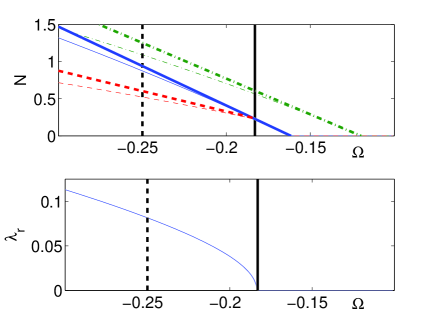
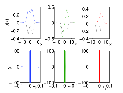
Figure 3: (Color Online) The figure shows the typical numerical bifurcation results for the cubic case and their comparison with the finite dimensional analysis of Section 3. Panel (a) shows the bifurcation diagram in the top subplot and the relevant real eigenvalues in the bottom subplot. In the top, the solid (blue) line represents the symmetric branch, the dash-dotted (green) line the anti-symmetric branch, while the dashed (red) line represents the bifurcating asymmetric branch. The thin lines indicate the numerical findings, while the thick ones show the corresponding finite-dimensional, weakly nonlinear predictions. The solid vertical (black) line indicates the critical point (of $\Omega\approx-0.1835$) obtained numerically. The dashed vertical (black) line is a guide to the eye for the case with $\Omega=-0.25$, whose detailed results are shown in panel (b). The bottom subplot of panel (a) shows the real eigenvalue (as a function of $\Omega$) of the symmetric branch that becomes unstable for $\Omega<-0.1835$. Panel (b) shows using the same symbolism as panel (a) the symmetric (left), anti-symmetric (middle) and asymmetric (right) branches and their linearization eigenvalues (bottom subplots) for $\Omega=-0.25$. The potential is shown by a dotted black line.

Symmetry breaking threshold, ${\cal N}_{cr}(L)$ as $L$ varies

We now investigate the limits of validity of ${\cal N}_{cr}^{(0)}(L)$ as an approximation to ${\cal N}_{cr}(L)$ by varying the distance $L$ between the potential wells (6.1). For $L$ large, ${\cal N}_{cr}^{(0)}$, given by equation (3.10), is close to the actual ${\cal N}_{cr}(L)$, the exact threshold. In this case the eigenvalues of $-\partial_{x}^{2}+V_{L}(x)$, $\Omega_{0}(L)$ and $\Omega_{1}(L)$, are close to each other; see Remark 4.1. Therefore, the bifurcation occurs for small ${\cal N}$ and one is in the regime of validity of Theorem 4.1. In figure 4 we display a comparison between the estimate for ${\cal N}_{cr}$ based on the finite dimensional truncation, ${\cal N}^{(0)}_{cr}$, and the actual ${\cal N}_{cr}$. For large $L$ the two values are close to each other. As $L$ is decreased the wells approach one another and eventually, at $L=0$, merge to form a single well potential. As $L$ is decreased, the eigenvalues of the linear bound states $\Omega_{0}(L)$ and $\Omega_{1}(L)$ move farther apart. For some value of $L$, $L_{d}$, the eigenvalue of the excited state, $\Omega_{1}(L)$, merges at $\Omega=0$, into the continuous spectrum. For $L<L_{d}$ the estimate ${\cal N}^{(0)}_{cr}$ is not correct. In fact, ${\cal N}_{cr}^{(0)}(L)\to\infty$, while the actual value of ${\cal N}_{cr}(L)$ appears to be remain finite. In Figure 4a we observe that for $L<2$, ${\cal N}^{(0)}$ and ${\cal N}_{cr}$ diverge from one another and eventually the approximation ${\cal N}^{(0)}_{cr}(L)$ tends to infinity, while the actual ${\cal N}_{cr}(L)$ remains finite. Moreover, in Figure 4b we show a bifurcation diagram for small $L$ in which the discrete (excited state) eigenvalue of $-\partial_{x}^{2}+V_{L}$, $\Omega_{1}$, does not exist, and yet there exists a symmetry breaking point ${\cal N}_{cr}$.

(a)	(b)

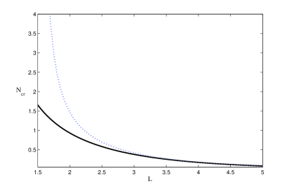
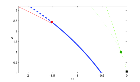
Figure 4: (Color Online) The figure demonstrates the validity of ${\cal N}_{cr}^{(0)}(L)$ as an approximation to ${\cal N}_{cr}(L)$. Panel (a) compares the linear finite dimensional estimation for the bifurcation point ${\cal N}^{(0)}_{cr}(L)$ and the actual numerical bifurcation point ${\cal N}_{cr}$. The computations are for the double well potential (6.1) $V_{0}=-1$ and $s=\frac{1}{4}$ and cubic nonlinearity. The curve ${\cal N}_{cr}(L)$ is marked by a solid (black) line and the curve ${\cal N}^{(0)}_{cr}(L)$ is marked by a dotted (blue) line. Panel (b) shows a numerical bifurcation diagram for the double well potential (6.1) $V_{0}=-1$, $s=\frac{1}{4}$ and $L=1.3$. The bifurcation point ${\cal N}_{cr}$ is marked by a (red) circle. For ${\cal N}<{\cal N}_{cr}$ the ground state marked by a thick (blue) solid line is stable. For ${\cal N}>{\cal N}_{cr}$ the ground state is unstable and marked by a thick (blue) dashed line. The stable asymmetric state which appears for ${\cal N}>{\cal N}_{cr}$ is marked by a thin (red) solid line. The unstable antisymmetric state $(\Omega^{{\cal N}}_{1})$ is marked by a thin (light green) dashed line. The point ${\cal N}$ for which the antisymmetric state appears in the discrete spectrum is marked by a (black) square. Notice that in this bifurcation diagram there is also a bifurcation from the antisymmetric branch. The state which bifurcates from the antisymmetric state is marked by a (dark green) thin dotted line.

More general nonlinearities

To simplify the analysis, we assumed a cubic nonlinearity in NLS-GP. The analogue of the finite-dimensional approximation (3.8) can be derived, for more general nonlinearities, by the same method. In this section we present numerical computations for general power law nonlinearities such as $K[\psi\bar{\psi}]=(\psi\bar{\psi})^{p}$ and observe similar phenomena to the cubic case $p=1$. This is illustrated e.g. in Figure 5, presenting our numerical results for the quintic case of $p=2$ (the relevant curves are analogous to those of Figure 3). It can be observed that the higher order case possesses a similar bifurcation diagram as the cubic case. However, the critical point for the emergence of the asymmetric branch is now shifted to $\Omega_{cr}^{(0)}\approx-0.1725$, i.e., considerably closer to the linear limit. In fact, we have also examined the septic case of $p=3$, finding that the relevant critical point is further shifted in the latter to $\Omega_{cr}^{(0)}=-0.168$. This can be easily understood as cases with higher $p$ are well-known to be more prone to collapse-type instabilities (see e.g. [25]). It may be an interesting separate venture to identify $\Omega_{cr}^{(0)}$ as a function of $p$, and possibly obtain a $p_{\star}$ such that $\forall\Omega<\Omega_{0}$, the symmetric branch is unstable. We also note in passing that bifurcation diagrams for higher values of $p$ may also bear additional (to the shift in $\Omega_{cr}^{(0)}$) differences from the cubic case; one such example in Figure 5 is given by the presence of a linear instability (due to a complex eigenvalue quartet emerging for $\Omega<-0.224$) for the anti-symmetric branch. The latter was found to be linearly stable in the cubic case of Fig. 3.

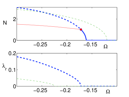
Figure 5: Same as Figure 3 but for the quintic nonlinearity. This serves to illustrate the analogies between the bifurcation pictures but also their differences (shifted critical point and also partial instability of the anti-symmetric branch).

Nonlocal nonlinearities

Finally, we consider the case of nonlocal nonlinearities, depending on a parameter $\epsilon$, the range of the nonlocal interaction. In particular, consider the case of a non-local nonlinearity of the form:

$$K[\psi\bar{\psi}]=\int_{-\infty}^{\infty}{\cal K}(x-y)\psi(y)\bar{\psi}(y)dy,$$ (6.3)

where

$${\cal K}(x-y)=\frac{1}{2\pi\epsilon^{2}}e^{-\frac{(x-y)^{2}}{2\epsilon^{2}}}.$$ (6.4)

Here, $\epsilon>0$ is a parameter controlling the range of the non-local interaction. As $\epsilon$ tends to $0$, ${\cal K}(x-y)\rightarrow\delta(x-y)$ and we recover the “local” cubic limit. limit. The form of the finite dimensional reduction, (3.8), does not change; the only modification is that the coefficients $a_{klmn}$ are now functions of the range of the interaction $\epsilon$. The dependence of the coefficients, $a_{klmn}$ on $\epsilon$ is displayed in panel (a) of Fig. 6. The solid (blue) line shows $|a_{0000}|$, the dashed (green) one corresponds to $|a_{1111}|$, the dash-dotted (red) one to $|a_{1001}|=|a_{0110}|$ (due to symmetry), while the thick solid (black) one to $|a_{0101}|=|a_{0011}|=|a_{1010}|$. Notice in the inset how the coefficients asymptote smoothly to their “local” limit. Additionally, note the expected asymptotic relation $a_{1001}=a_{0011}$. Also note the significant (decaying) dependence of the relevant coefficients on the range of the interaction. The nature of this dependence indicates that while the character of the bifurcation may be the same as in the case of local nonlinearities, its details (such as the location of the critical points) depend sensitively on the range of the non-local interaction. This is illustrated in panel (b) for the specific case of $\epsilon=5$. In this panel (which is analogous to panel (a) of Figure 3, but for the non-local case) the critical point for emergence of the asymmetric branch/instability of the symmetric branch is shifted to $\Omega_{cr}^{(0)}=-0.2466$ (and the corresponding ${\cal N}_{cr}=1.4353$) in comparison to the numerically obtained value of $\Omega_{cr}^{(0)}\approx-0.256$; the relative error in the identification of the critical point (by the finite-dimensional reduction) is in this case of the order of $3.7\%$, which can be attributed to the more strongly nonlinear (i.e., occurring for higher value of ${\cal N}_{cr}^{(0)}$) nature of the bifurcation. However, as the finite-dimensional approximation still yields a reliable estimate for the location of the critical point, in panel (c) we use it to obtain an approximation to the location of the critical point $(\Omega_{cr}^{(0)},{\cal N}_{cr}^{(0)})$ as a function of the non-locality parameter $\epsilon$.

(a)	(b)

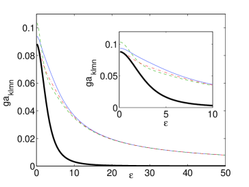
(c)

Figure 6: This figure shows the nonlocal analog of Figure 3. Panel (a) shows the dependence of the (absolute value of the) coefficients of the finite-dimensional approximation on the non-locality parameter $\epsilon$ ($\epsilon=0$ denotes the “local” nonlinearity limit). The solid (blue) line denotes $a_{0000}$, the dashed (green) $a_{1111}$, the dash-dotted (red) $a_{0110}$, while the thick solid (black) one denotes $a_{0101}$. Panel (b) is analogous to panel (a) of Figure 3, but now shown for the non-local case, with the non-locality parameter $\epsilon=5$. Finally, panel (c) shows the dependence of the critical point of the finite dimensional bifurcation $(N_{\star},\Omega_{\star})$, on the non-locality parameter $\epsilon$.

7 Concluding remarks

We have studied the spontaneous symmetry breaking for a large class of NLS-GP equations, with double-well potentials. Our analysis of the symmetry breaking bifurcation and the exchange of stability is based on an expansion, which to leading order in amplitude, is a superposition of a symmetric - antisymmetric pair of eigenstates of the linear Hamiltonian, $H$, whose energies are separated (gap condition (4.7) ) from all other spectra of $H$. This gap condition holds for sufficiently large $L$ but breaks down as $L$ decreases. Nevertheless, numerical studies show the existence of a finite threshold for symmetry breaking. A theory encompassing this phenomenon is of interest and is currently under investigation.

8 Appendix - Double wells

In this discussion, we are going to follow the analysis of [8]. Consider a (single well) real valued potential $v_{0}(x)$ on $\mathbb{R}^{n}$ such that $v_{0}(x)\in L^{r}+L^{\infty}_{\varepsilon}$ for all $1\leq r\leq q$ where $q\geq\max(n/2,2)$ for $n\not=4,$ $q>2$ for $n=4.$ Then, multiplication by $v_{0}$ is a compact operator from $H^{2}$ to $L^{2}$ and

$$H_{0}=-\Delta+v_{0}(x)$$

is a self adjoint operator on $L^{2}$ with domain $H^{2}.$

Consider now the double well potential:

$$V_{L}=T_{L}v_{0}T_{-L}+RT_{L}v_{0}T_{-L}R$$

where $T_{L}$ and $R$ are the unitary operators:

$$T_{L}g(x_{1},x_{2},\ldots,x_{n}) = g(x_{1}+L,x_{2},\ldots,x_{n})$$

$$Rg(x_{1},x_{2},\ldots,x_{n}) = g(-x_{1},x_{2},\ldots,x_{n})$$

and the self adjoint operator:

$$H_{L}=-\Delta+V_{L}(x)$$

Proposition 8.1

Assume that $\omega<0$ is a nondegenerate eigenvalue of $H_{0}$ separated from the rest of the spectrum of $H_{0}$ by a distance greater than $2d_{*}.$ Denote by $\psi_{\omega}$ its corresponding e-vector, $\|\psi_{\omega}\|_{L^{2}}=1.$ Then there exists $L_{0}>0$ such that for $L\geq L_{0}$ the following are true:

• $H_{L}$ has exactly two eigenvalues $\Omega_{0}(L)$ and $\Omega_{1}(L)$ nearer to $\omega$ than $2d_{*}.$ Moreover $\lim_{L\rightarrow\infty}\Omega_{j}(L)=\omega,\ j=0,1.$

• One can choose the normalized eigenvectors $\psi_{j}(L),\ \|\psi_{j}(L)\|_{L^{2}}=1,$ corresponding to the e-values $\Omega_{j}(L),\ j=0,1$ such that they satisfy:

  $$\lim_{L\rightarrow\infty}\|\psi_{j}(L)-(T_{L}\psi_{\omega}+(-1)^{j}RT_{L}\psi_{\omega})/\sqrt{2}\|_{H^{2}}=0,\ j=0,1.$$

• If $P^{L}_{j}$ are the orthogonal projections in $L^{2}$ onto $\psi_{j}(L),\ j=0,1$ and $\tilde{P}_{L}=Id-P^{L}_{0}-P^{L}_{1}$ then there exists $d>0$ independent of $L$ such that:

  $$\|(H_{L}-\Omega)^{-1}\tilde{P}_{L}\|_{L^{2}\mapsto H^{2}}\geq d,\quad{\rm for\ all}\ L\geq L_{0}\ {\rm and}\ |\Omega-\omega\|\leq d_{*}.$$

Proof: For (i) we refer the reader to [8]. The $L^{2}$ convergence in (ii) has also been proved there. The $H^{2}$ convergence follows from the following compactness argument. Let:

$$\psi^{L}_{j}=n_{L}\psi_{j}(L),\qquad j=0,1$$

where $n_{L}$ is such that $\|\psi^{L}_{j}\|_{H^{2}}=1,\ j=0,1.$ From the eigenvector equations: $(H_{L}-\Omega(L))\psi^{L}=0,$ where we dropped the index $j=0,1$ and the convergence $\Omega(L)\rightarrow\omega,$ see part (i), we get

$$\lim_{L\rightarrow\infty}\|(-\Delta-\omega+V_{L})\psi^{L}\|_{L^{2}}=0.$$ (8.1)

Denote:

$$g_{L}=(-\Delta-\omega)\psi^{L}\in L^{2}.$$ (8.2)

Since $-\Delta-\omega:H^{2}\mapsto L^{2}$ is bounded there exists a constant $C>0$ independent of $L$ such that

$$\|g_{L}\|_{L^{2}}\leq C.$$

Since $\omega<0,$ $-\Delta-\omega:H^{2}\mapsto L^{2}$ has a continuous inverse then (8.1) is equivalent to:

$$g_{L}+V_{L}(-\Delta-\omega)^{-1}g_{L}\rightarrow 0,\ {\rm in}\ L^{2}.$$

By expanding $V_{L}$ we get

$$g_{L}+T_{L}v_{0}(-\Delta-\omega)^{-1}T_{-L}g_{L}+RT_{L}v_{0}(-\Delta-\omega)^{-1}T_{-L}Rg_{L}\rightarrow 0.$$ (8.3)

But $v_{0}(-\Delta-\omega)^{-1}:L^{2}\mapsto L^{2}$ is compact while the translation and reflection operators are unitary. These and the uniform boundedness of $g_{L}$ lead to the existence of $\psi\in L^{2}$ and $\tilde{\psi}\in L^{2}$ and a subsequence of $g_{L},$ which we will redenote by $g_{L},$ such that

$$\lim_{L\rightarrow\infty}\|v_{0}(-\Delta-\omega)^{-1}T_{-L}g_{L}-\psi\|_{L^{2}}=0\ {\rm and}\ \lim_{L\rightarrow\infty}\|v_{0}(-\Delta-\omega)^{-1}T_{-L}Rg_{L}-\tilde{\psi}\|_{L^{2}}=0.$$ (8.4)

By plugging in (8.3) and multiplying to the left by $T_{-L}$ we get

$$\lim_{L\rightarrow\infty}\|T_{-L}g_{L}+\psi+RT_{2L}\tilde{\psi}\|_{L^{2}}=0.$$

But $RT_{2L}\tilde{\psi}$ converges weakly to zero, hence $T_{-L}g_{L}$ converges weakly to $-\psi.$ By plugging now in (8.4) and using compactness we get:

$$\psi+v_{0}(-\Delta-\omega)^{-1}\psi=0.$$

The latter shows that $(-\Delta-\omega)^{-1}\psi$ is an eigenvector of $-\Delta+v_{0}$ corresponding to the eigenvalue $\omega.$ By nondegeneracy of $\omega$ we get

$$\psi=-n(-\Delta-\omega)\psi_{\omega},$$ (8.5)

where $n$ is a constant. A similar argument shows

$$\tilde{\psi}=-\tilde{n}(-\Delta-\omega)\psi_{\omega},$$ (8.6)

where $\tilde{n}$ is a constant.

Combining (8.1)-(8.6) we get

$$\lim_{L\rightarrow\infty}\|(-\Delta-\omega)(\psi^{L}-nT_{L}\psi_{\omega}-\tilde{n}RT_{L}\psi_{\omega})\|_{L^{2}}=0$$ (8.7)

which by the continuity of $(-\Delta-\omega)^{-1}:L^{2}\mapsto H^{2}$ implies

$$\lim_{L\rightarrow\infty}\|\psi^{L}-nT_{L}\psi_{\omega}-\tilde{n}RT_{L}\psi_{\omega}\|_{H^{2}}=0$$

Using now that $\|\psi^{L}\|_{H^{2}}=1$ and that the rescaled $\psi_{j}^{L}$ such that it has norm 1 in $L^{2}$ converges to $(T_{L}\psi_{\omega}+(-1)^{j}RT_{L}\psi_{\omega})/\sqrt{2}$ we get the conclusion of part (ii) for a subsequence first, then, by uniqueness of the limit, for all $L\rightarrow\infty.$

For part (iii), it suffices to show that there are no sequences $(\Omega_{L},\psi^{L})\in[\omega-d_{*},\omega+d_{*}]\times H^{2}$ with $\|\psi^{L}\|_{H^{2}}=1$ and $\psi_{L}\bot\psi_{j}(L),\ j=0,1$ in $L^{2}$ such that

$$\lim_{L\rightarrow\infty}\|(H_{L}-\Omega_{L})\psi^{L}\|_{L^{2}}=0.$$ (8.8)

The spectral estimate:

$$\|(H_{L}-\Omega_{L})\psi^{L}\|_{L^{2}}\geq dist(\Omega_{L},\sigma(H_{L})\backslash\{\Omega_{0}(L),\Omega_{1}(L)\})\|\psi^{L}\|_{L^{2}}\geq d_{*}\|\psi^{L}\|_{L^{2}},$$

combined with (8.8) implies

$$\lim_{L\rightarrow\infty}\|\psi^{L}\|_{L^{2}}=0.$$ (8.9)

In principle we can now employ the compactness argument in part (ii) to get

$$\lim_{L\rightarrow\infty}\|\psi^{L}\|_{H^{2}}=0$$ (8.10)

which will contradict $\|\psi^{L}\|_{H^{2}}=1.$ More precisely, (8.8)-(8.9) imply

$$\lim_{L\rightarrow\infty}\|(-\Delta-\omega-d_{*}+V_{L})\psi^{L}\|_{L^{2}}=0$$

which, by repeating the argument after (8.1) with $\omega$ replaced by $\omega+d_{*}$, gives

$$\lim_{L\rightarrow\infty}\|\psi^{L}+T_{L}\psi_{\omega+d_{*}}+RT_{L}\tilde{\psi}_{\omega+d_{*}}\|_{H^{2}}=0$$

where $\psi_{\omega+d_{*}}$ and $\tilde{\psi}_{\omega+d_{*}}$ are eigenvectors of $-\Delta+v_{0}$ corresponding to eigenvalue $\omega+d_{*}.$ But the latter is not actually an eigenvalue, hence $\psi_{\omega+d_{*}}=0$ and $\tilde{\psi}_{\omega+d_{*}}=0.$ These show (8.10) and finishes the proof of part (iii).

The proposition is now completely proven.

Proposition 8.2

$$a_{1001}+2a_{1010}-a_{0000}\ \leq-\gamma<0,\ \ \ {\rm and}$$ (8.11)

$$\frac{\Omega_{1}-\Omega_{0}}{|a_{1001}+2a_{1010}-a_{0000}|^{2}}\to 0\ {\rm as}\ L\uparrow\infty,$$ (8.12)

These are now obvious from definition of $a_{ijkl}$, the continuity of $N:H^{2}\times H^{2}\times H^{2}\mapsto L^{2}$ and the $H^{2}$ convergence of $\psi_{j}(L)$ to the translations and reflections of the single well eigenvector, see Proposition 8.1 part (ii).

References

[1]
M. Albiez, R. Gati, J. Fölling, S. Hunsmann, M. Cristiani, and M.K.
Oberthaler.
Direct observation of tunneling and nonlinear self-trapping in a
single bosonic josephson junction.
Phys. Rev. Lett., 95:010402, 2005.
[2]
W.H. Aschbacher, J. Fröhlich, G.M. Graf, K. Schnee, and M. Troyer.
Symmetry breaking regime in the nonlinear hartree equation.
J. Math. Phys., 43:3879–3891, 2002.
[3]
C. Cambournac, T. Sylvestre, H. Maillotte, B. Vanderlinden, P. Kockaert, Ph.
Emplit, and M. Haelterman.
Symmetry-breaking instability of multimode vector solitons.
Phys. Rev. Lett., 89:083901, 2002.
[4]
B. Deconinck and J. Nathan Kutz.
Singular instability of exact stationary solutions of the nonlocal
gross-pitaeskii equation.
Phys. Lett. A, 319:97–103, 2003.
[5]
Jason Fleischer, Guy Bartal, Oren Cohen, Tal Schwartz, Ofer Manela, Barak
Freedman, Mordechai Segev, Hrvoje Buljan, and Nikolaos Efremidis.
Spatial photonics in nonlinear waveguide arrays.
Optics Express, 13(6):1780–1796, March 2005.
[6]
M.G. Grillakis.
Linearized instability for nonlinear Schrödinger and
Klein-Gordon equations.
Comm. Pure Appl. Math., 41:747–774, 1988.
[7]
M.G. Grillakis, J. Shatah, and W.A. Strauss.
Stability theory of solitary waves in the presence of symmetry i.
J. Funct. Anal., 74(1):160–197, 1987.
[9]
T. Heil, I. Fischer, and W. Elsässer.
Chaos synchronization and spontaneous symmetry-breaking in
symmetrically delay-coupled semiconductor lasers.
Phys. Rev. Lett., 86:795–798, 2001.
[10]
R.K. Jackson and M.I. Weinstein.
Geometric analysis of bifurcation and symmetry breaking in a
Gross-Pitaevskii equation.
J. Stat. Phys., 116:881–905, 2004.
[11]
C.K.R.T. Jones.
An instability mechanism for radially symmetric standing waves of a
nonlinear Schrödinger equation.
J. Diff. Equa., 71:34–62, 1988.
[12]
T. Kapitula.
Stability of waves in perturbed Hamiltonian systems.
Physica D, 156:186–200, 2001.
[13]
T. Kapitula and P. Kevrekidis.
Bose-einstein condensates in the presence of a magnetic trap and
optical lattice: two-mode approximation.
Nonlinearity, 18(6):2491–2512, 2005.
[14]
T. Kapitula, P.G. Kevrekidis, and Z. Chen.
Three is a crowd: Solitary waves in photorefractive media with three
potential wells.
to appear in SIAM J. Appl. Dyn. Sys.
[15]
T. Kapitula, P.G. Kevrekidis, and B. Sandstede.
Counting eigenvalues via the krein signature in infinite-dimensional
hamiltonian systems.
Physica D, 195:263–282, 2004.
[16]
P.G. Kevrekidis, Z. Chen, B.A. Malomed, D.J. Frantzeskakis, and M.I. Weinstein.
Spontaneous symmetry breaking in photonic lattices: Theory and
experiment.
Phys. Lett. A, 340:275–280, 2005.
[17]
W. Krolikowski, O. Bang, N.I. Nikolov, D. Neshev, J. Wyller, J.J. Rasmussen,
and D. Edmundson.
Modulational instability, solitons and beam propagation in spatially
nonlocal nonlinear media.
J. Opt. B: Quantum Semiclass. Opt., 6:S288–S294, 2004.
[18]
K.W. Mahmud, J.N. Kutz, and W.P. Reinhardt.
Bose-einstein condensates in a one-dimensional double square well:
Analytical solutions of nonlinear schrödinger equation.
Phys. Rev. A, 66:063607, 2002.
[19]
L. Nirenberg.
Lectures on Nonlinear Functional Analysis.
Courant Institute, New York, 1974.
[20]
Claude-Alain Pillet and C. Eugene Wayne.
Invariant manifolds for a class of dispersive, Hamiltonian.
J. Differential Equations, 141(2):310–326, 1997.
[21]
H.A. Rose and M.I. Weinstein.
On the bound states of the nonlinear Schrödinger equation with a
linear potential.
Physica D, 30:207–218, 1988.
[22]
A. Sacchetti.
Nonlinear time-dependent one-dimensional schrödinger equation
with double-well potential.
SIAM J. Math. Anal., 35:1160–1176, 2003.
[23]
S. Sawai, Y. Maeda, and Y. Sawada.
Spontaneous symmetry breaking turing-type pattern formation in a
confined dictyostelium cell mass.
Phys. Rev. Lett., 85:2212–2215, 2000.
[24]
A.G. Vanakaras, D.J. Fotinos, and E.T. Samulski.
Tilt, polarity, and spontaneous symmetry breaking in liquid crystals.
Phys. Rev. E, 57:R4875–R4878, 1998.
[25]
M.I. Weinstein.
Modulational stability of ground states of nonlinear Schrödinger
equations.
SIAM J. Math. Anal., 16:472–491, 1985.
[26]
M.I. Weinstein.
Lyapunov stability of ground states of nonlinear dispersive evolution
equations.
Comm. Pure Appl. Math., 39:51–68, 1986.
[27]
C. Yannouleas and U. Landman.
Spontaneous symmetry breaking in single and molecular quantum dots.
Phys. Rev. Lett., 82:5325–5328, 1999.