Complex trajectories in chaotic dynamical tunneling

Abstract

We develop the semiclassical method of complex trajectories in application to chaotic dynamical tunneling. First, we suggest a systematic numerical technique for obtaining complex tunneling trajectories by the gradual deformation of the classical ones. This provides a natural classification of the tunneling solutions. Second, we present a heuristic procedure for sorting out the least suppressed trajectory. As an illustration, we apply our technique to the process of chaotic tunneling in a quantum mechanical model with two degrees of freedom. Our analysis reveals rich dynamics of the system. At the classical level, there exists an infinite set of unstable solutions forming a fractal structure. This structure is inherited by the complex tunneling paths and plays the central role in the semiclassical study. The process we consider exhibits the phenomenon of optimal tunneling: the suppression exponent of the tunneling probability has a local minimum at a certain energy which is thus (locally) the optimal energy for tunneling. We test the proposed method by comparison of the semiclassical results with the results of the exact quantum computations and find a good agreement.

I Introduction

An intrinsic feature of quantum physics is the existence of processes which are forbidden at the classical level. The text–book examples of such processes are tunneling and over–barrier reflection in one–dimensional quantum mechanics; more involved topics include atom ionization processes Perelomov , chemical reactions Miller , false vacuum decay in scalar field theory Coleman:1977py , etc. Generically, one introduces a certain parameter $g^{2}$ (the Planck constant $\hbar$ in quantum mechanics, coupling constant in field theory, etc.) measuring the magnitude of quantum fluctuations, and finds that the probabilities ${\cal P}$ of classically forbidden processes behave exponentially as $g^{2}\to 0$,

$${\cal P}\simeq g^{\gamma}A{\rm e}^{-F/g^{2}}\;.$$ (1)

Here $F>0$ is the suppression exponent and the dependence of the pre-exponential factor on $g$ is indicated explicitly. In this paper we adopt the term “tunneling” for any process forbidden at the classical level. This includes, in particular, the cases of dynamical tunneling Miller ; Heller:1981 , when the exponential suppression of the process is not related to the existence of a potential barrier.

A powerful tool for the study of tunneling at small $g^{2}$ is provided by the semiclassical methods. Exploiting the semiclassical approach, one reduces the problem of computing the tunneling probability to the problem of finding the relevant solution to the classical equations of motion in the complex domain Perelomov ; Miller ; Wilkinson:Takada , where both the time variable $t$ and dynamical coordinates are taken to be complex. The suppression exponent $F$ is then related to the classical action $S$ calculated along an appropriate contour in the complex time plane. The shape of this contour, as well as the boundary conditions imposed on the solution at $t\to\pm\infty$, are dictated by the quantum numbers of the initial and final states. In the simplest cases of under–barrier motion (one-dimensional tunneling, false vacuum decay) the contour runs along the imaginary time axis, and the relevant solution is real along this axis. Such a trajectory may be identified with the “most probable escape path” in the configuration space Banks:1973ps ; Coleman:1977py , which gives some understanding of the classically forbidden dynamics. In other cases, however, the passage of the system through the classically forbidden region of the phase space cannot be treated separately from the preceding and following real–time evolution, and the analysis of complex tunneling solutions in the complex time domain is needed. This happens, e.g., in the study of chemical reactions with definite initial quantum state of reactants Miller or in the investigation of the induced tunneling processes in field theory Rubakov:1992ec ; Kuznetsov:1997az ; Bezrukov:2003er ; Levkov:2004tf . The semiclassical techniques based on genuinely complex classical solutions received the common name of the method of complex trajectories.

It should be pointed out that the application of the above method might be highly non–trivial. Major complications are related to the issues of existence and uniqueness of tunneling trajectories, which are basically the complex solutions to a certain boundary value problem. First, it may occur that the boundary value problem at hand does not have any solutions at all (see, e.g., Ref. Affleck:1980mp ). Second, there may exist many (sometimes an infinite number of) solutions. Some of them may well be unphysical and should be rejected. The identification of physical solutions relies very much on the particular properties of the system under consideration; presently there are no trustworthy criteria applicable in general (see Refs. Berry:1972 ; Adachi:1986 ; Shudo:1996 ; Ribeiro:2004 ; Parisio:2005 for the attempts to find such criteria). Even after the unphysical solutions are eliminated, the problem remains to identify the solution(s) which yield the minimal suppression exponent and therefore correspond to the dominant contribution to the tunneling amplitude.

The above difficulties become particularly pronounced in the case of tunneling in chaotic systems. Appearance of chaos is generic for non–linear systems with many degrees of freedom; the topics related to tunneling in the presence of chaos were addressed in Refs. Adachi:1986 ; Bohigas1993 ; Doron1995 ; Mouchet2001 ; Shudo1995_1 ; Shudo:1996 ; Shudo2002 ; Onishi2003 ; Ribeiro:2004 . The semiclassical analysis of chaotic tunneling is hindered by the existence of an infinite number of semiclassical solutions which form a fractal set in the complex phase space Adachi:1986 ; Shudo1995_1 ; Onishi2003 . The direct analysis of this set with the purpose of identifying the physically relevant solutions becomes an elaborative task in the systems with many degrees of freedom Heller2002 . Presently, the semiclassical analysis of the chaotic tunneling processes is limited to the special cases when the phase space of the system can be explicitly visualized Adachi:1986 ; Shudo1995_1 ; Onishi2003 , or when the small sub–class of periodic tunneling orbits is considered Ribeiro:2004 . Development of generic methods of classifying the semiclassical solutions is of great importance Heller2002 .

In this paper we present new method of obtaining and classifying the tunneling trajectories, which is applicable, in particular, in the case of many–dimensional ($D\geq 2$) chaotic tunneling. Namely, we consider the processes which proceed classically at some values of the initial-state quantum numbers, and become exponentially suppressed at other values. The technique presented below enables one to obtain complex trajectories describing tunneling by starting from the real classical solutions and changing gradually the quantum numbers of the initial state. Our procedure has two advantages. First, it is generic and numerically implementable. Second, it provides a natural classification of tunneling trajectories based on the analysis of their classical progenitors. The latter classification suggests a heuristic method for sorting out the least suppressed tunneling path.

As an illustration we apply the above method to the problem of scattering in quantum mechanical model with two degrees of freedom. The process we study is a particular exemple of over-barrier reflection. We calculate the suppression exponent for the reflection probability. As the test of the method we compare the semiclassical results with the “exact” suppression exponent. The latter is extracted from the exact wave function obtained by solving numerically the Schrödinger equation. The results of the two calculations are in good agreement.

The system under consideration has two distinctive features, which are inherent in two wide (intersecting but not necessarily identical) classes of tunneling problems. We believe that our model is a generic representative of both of these classes.

The first feature is chaoticity. In our model chaos manifests itself at the classical level as follows. Consider the set of initial data giving rise to the classical reflected trajectories. We will see that this set falls into an infinite number of disconnected domains. The boundaries of these domains correspond to trajectories which do not escape into the final asymptotic region as time goes on, but get trapped in the interaction region. The latter trajectories are unstable: small deviations from them lead to either reflected or transmitted solutions. Increasing the resolution of initial data reveals that the set of initial data corresponding to the trapped trajectories forms a fractal similar to the Cantor set. This is the hallmark of the so–called irregular (or chaotic) scattering Eckhardt1986 .

The chaoticity of the classical dynamics has profound consequences for the tunneling process. We will show that complex trajectories relevant for over–barrier reflection are all trapped in the interaction region and thus are unstable. Moreover, they inherit the fractal structure of the classical trapped solutions which means, in particular, that their number is infinite. The complex trajectory which contributes most to the tunneling amplitude is a descendant of a certain unstable classical solution lying on the boundary of the above fractal set.

The chaoticity of the process manifests itself in the exact quantum computations as well. We find that the quantum probability of tunneling, instead of being smooth function of energy, exhibits large irregular oscillations. Similar dependence of the tunneling amplitude on the parameters of chaotic systems was reported previously in Refs. Bohigas1993 ; Doron1995 ; Shudo1995_1 . At first glance, this behavior contradicts to the semiclassical formula (1). One observes, however, that the oscillation period scales like $g^{2}$ when $g^{2}\to 0$, so that the oscillations become indiscernible in the semiclassical limit. In order to extract the semiclassical suppression exponent, one smears the tunneling probability over several periods. The smeared probability does obey the scaling law (1).

The second feature of our system is as follows. We observe that the process under consideration is classically forbidden, and hence exponentially suppressed, at arbitrary high energies. Our interest in this property is motivated by the studies of similar processes in quantum field theory. As a matter of fact, the exponential suppression at all energies is generic for the field theoretical processes involving creation of some classical object (soliton, bubble of new phase or vacuum configuration with different topology) in a collision of two highly energetic quantum particles Zakharov:1990xt ; Maggiore:1991kh ; Voloshin:1993dk ; Rubakov:1994hz ; Levkov:2004tf . Moreover, it has been shown recently Levkov:2004tf that the method of complex trajectories predicts the suppression exponent $F$ of the above processes to attain its minimum at a certain “optimal” energy $E_{o}$, above which $F$ stays constant (this behavior of the suppression exponent was conjectured earlier in Refs. Maggiore:1991kh ; Voloshin:1993dk ). The optimal value $F(E_{o})$ is determined by the complex–valued classical solutions with particular properties, see Refs Levkov:2004tf ; these solutions are called “real–time instantons”.

One might question the applicability of the method of complex trajectories for the description of the above phenomenon of optimal tunneling. Indeed, the properties of processes at $E\approx E_{o}$ are in many respects different from the well–known case of tunneling through a potential barrier. In this paper we provide the evidence that the semiclassical method is applicable for the description of dynamical tunneling independently of how high the energy of the process is, or whether there exists a potential barrier at all.

The model of this paper provides a particular example of quantum mechanical system exhibiting the phenomenon of optimal tunneling. Namely, the suppression exponent $F(E)$ depends on energy $E$ in non-monotonic way, attaining a local minimum at some energy $E_{o}$. We will find that the minimal value of the suppression exponent is indeed given by the method of real-time instantons. At higher energies the function $F(E)$ grows to infinity.

The paper is organized as follows. In Sec. II we describe the model under consideration and introduce notations. In Sec. III the classical dynamics of the system is analyzed. The semiclassical study of the classically forbidden reflections is performed in Sec. IV. In Sec. V we present the results of the numerical integration of the Schrödinger equation and discuss their comparison with the semiclassical results. Sec. VI contains summary and conclusions.

II Setup

Throughout the paper we illustrate our technique on a toy model describing the evolution of a quantum particle in two-dimensional harmonic waveguide. Namely, we consider the case when the motion of the particle is confined to the vicinity of a certain line $Y=\frac{1}{g}a(gX)$ by the quadratic potential ($X$ and $Y$ stand for the Cartesian coordinates of the particle). The equipotential contour ${\cal U}(X,Y)={\cal E}$ is shown in Fig. 1; the Hamiltonian is

Figure 1: The equipotential contour ${\cal U}(X,Y)={\cal E}$ for the waveguide model (2) and the directions of the incoming, reflected and transmitted fluxes of particles.

$${\cal H}=\frac{P_{X}^{2}+P_{Y}^{2}}{2m}+{\cal U}(X,Y)\;,$$ (2)

where

$${\cal U}(X,Y)=\frac{m\omega^{2}}{2}\left[Y-\frac{1}{g}a\!\left(gX\right)\right]^{2}\;,$$ (3)

$$a(x)=a_{0}{\rm e}^{-x^{2}/2}\;.$$

In the asymptotic regions $X\to\pm\infty$, the variables of the model (2) separate, and the motion of the particle becomes trivial: oscillations in the $Y$-direction are accompanied by the translatory motion along the $X$-axis. The wriggle around the point $X\approx 0$ introduces nonlinear coupling between the degrees of freedom; we refer to this part of the configuration space as the interaction region.

In what follows we use the system of units where

$$\hbar=\omega=m=1\;.$$ (4)

The rescaling

$${\boldsymbol{X}}={\boldsymbol{x}}/g\;,\qquad{\boldsymbol{P}}={\boldsymbol{p}}g$$ (5)

brings the Hamiltonian (2) into the form

$${\cal H}=\frac{g^{2}(p_{x}^{2}+p_{y}^{2})}{2}+\frac{1}{2g^{2}}(y-a(x))^{2}\;.$$ (6)

Equation (6) implies that the semiclassical regime in our model occurs for $g^{2}\ll 1$. Apart from $g^{2}$, the only free parameter of the model (6) is $a_{0}$, which we set

$$a_{0}=0.8\;.$$ (7)

This choice will be explained in Sec. III. To avoid confusion, we remark that the rescaled coordinates $x$, $y$ will be used for the semiclassical analysis of Secs. III, IV and App. A, while the original ones ($X$ and $Y$) are exploited in the quantum computations of Sec. V and App. B.

The process we want to investigate is the backward reflection of a particle coming from the right, see Fig. 1. Note that though we will refer to this process as over-barrier reflection, there is actually no potential barrier in our system: the minimum of the potential is zero in any transverse section of the waveguide. The incoming quantum state $|{\cal E},{\cal N}\rangle$ is completely determined by the total energy ${\cal E}$ and occupation number ${\cal N}$ of the $Y$-oscillator. The quantity of interest is the total reflection coefficient for this state,

$${\cal P}({\cal E},{\cal N})=\lim_{t_{f}-t_{i}\to+\infty}\frac{1}{t_{f}-t_{i}}\times\\ \times\sum_{f}\big{|}\langle f|{\rm e}^{-i{\cal H}(t_{f}-t_{i})}|{\cal E},{\cal N}\rangle\big{|}^{2}\;,$$ (8)

where $|f\rangle$ stands for the basis of reflected waves ($P_{f}>0$) supported in the right asymptotic region, and the proper normalization of the incoming state has been chosen,

$$\langle{\cal E},{\cal N}|{\cal E}^{\prime},{\cal N}^{\prime}\rangle=2\pi\delta({\cal E}-{\cal E}^{\prime})\delta_{{\cal NN}^{\prime}}\;.$$ (9)

At some values of the initial–state parameters ${\cal E}$, ${\cal N}$ the reflection process is classically forbidden. [In particular, one expects a particle with high enough translatory momentum $|P_{i}|$ to pass classically to the other side of the waveguide ending up in the asymptotic region $X\to-\infty$.] In this case the reflection coefficient (8) is expected to obey the semiclassical scaling law (1) at $g^{2}\to 0$. Below we concentrate on the calculation of the leading suppression exponent $F$ as function of ${\cal E}$, ${\cal N}$.

We do not pretend to describe any concrete experimental situation by the Hamiltonian (2); it is chosen as a convenient testing ground of our semiclassical technique. The advantage of the scattering setup is an unambiguous determination of the initial and final states of the tunneling process, the latter determination being problematic in the case of bounded motion Wilkinson:Takada . Moreover, the simple form of our model makes it tractable both semiclassically and by the exact quantum mechanical methods. Note that a system similar to (2) was considered in Ref. Drew2005 .

III Classical reflections

Let us start by considering the classical dynamics of the reflection process. As we will see in Sec. IV, the analysis of the classical dynamics is crucial for understanding the classically forbidden reflections. The results of the present Section will enable us to identify the sets of the initial data $({\cal E},\;{\cal N})$ which correspond to the classically allowed/forbidden reflections; for brevity we refer to these sets as classically allowed/classically forbidden regions. Note that these are the regions in the initial data plane $({\cal E},\,{\cal N})$; they should not be confused with the classically allowed/forbidden regions in the configuration space. The latter term is not used in this paper.

One notes that the action functional of the model (6) has the form

$${\cal S}=S/g^{2},$$ (10)

where

$$S=\int\left(\frac{\dot{x}^{2}+\dot{y}^{2}}{2}-\frac{1}{2}(y-a(x))^{2}\right)dt\;$$ (11)

does not contain the parameter $g$ at all. Hence, $g$ drops out of the classical equations of motion. While studying the classical dynamics it is convenient to forget about $g$ and consider the classical system defined by the rescaled action (11).

In contrast to quantum mechanics, where two quantum numbers ${\cal E}$, ${\cal N}$ determine the initial state completely, the classical evolution is specified by four initial conditions. One of these is physically irrelevant. It corresponds to the $x$ coordinate at the initial moment $t=t_{i}$, and can be absorbed by the appropriate shift of $t_{i}$. Note that, still, one should be careful to choose $x(t_{i})$ far from the interaction region; in numerical calculations of this Section the value

$$x(t_{i})=10$$ (12a)

is used. To keep contact with the quantum mechanical formulation we choose the other two initial data to be the total classical energy $$E N$$ and the “classical occupation number” , which is equal to the initial classical energy of the transverse oscillations. This determines the initial velocity of the particle along the waveguide,

$$\dot{x}(t_{i})=-\sqrt{2(E-N)}\;.$$ (12b)

It is worth noting that Eq. (10) implies the following relation between the classical parameters and their quantum counterparts,

$$E=g^{2}{\cal E}~{},\qquad N=g^{2}{\cal N}\;.$$ (13)

The last initial condition is the initial phase $\phi_{0}$ of $y$-oscillator. It parametrizes the initial position and velocity of the particle in the transverse section of the waveguide:

$$y(t_{i})=\sqrt{2N}\cos\phi_{0}\;,$$ (14a)

$$\dot{y}(t_{i})=-\sqrt{2N}\sin\phi_{0}\;.$$ (14b)

Clearly, a given point of the plane $(E,N)$ belongs to the classically allowed region if classical reflection is possible for some value(s) of $\phi_{0}$. Otherwise, we say that this point lies in the classically forbidden region.

At first glance it may seem that classical reflections are impossible for any values of $E$, $N$ as there is no potential barrier to prevent the classical particle from going into the left asymptotic region. Let us make sure that this is not the case by considering the evolution at small $E$. In this regime the particle moves slowly along the axis $y=a(x)$ of the waveguide performing small and (relatively) rapid oscillations in the orthogonal direction. The frequency $\omega_{\perp}$ of the latter oscillations is determined by the curvature of the transverse section of the potential and thus depends on the position $x$ of the particle. It is straightforward to find that $\omega_{\perp}(x)=\sqrt{1+(a^{\prime}(x))^{2}}$. The energy of the orthogonal oscillations $E_{\perp}$ divided by their frequency is an adiabatic invariant,

$$\frac{E_{\perp}}{\omega_{\perp}(x)}=const=N\;.$$ (15)

On the other hand, the conservation of total energy yields,

$$E=\frac{v_{\parallel}^{2}}{2}+E_{\perp}=\frac{v_{\parallel}^{2}}{2}+N\sqrt{1+(a^{\prime}(x))^{2}}\;,$$ (16)

where $v_{\parallel}$ is the projection of the particle velocity onto the axis of the waveguide. Thus, the adiabatic motion in our waveguide is governed by one–dimensional dynamics in the effective potential

$$U(x)=N\sqrt{1+a_{0}^{2}x^{2}{\rm e}^{-x^{2}}}\;.$$ (17)

where the explicit expression (3) for the function $a(x)$ has been used. This picture is valid as long as $\dot{\omega}_{\perp}/\omega_{\perp}^{2}\ll 1$, which is satisfied for $E,N\ll 1$.

The potential (17) has the form of two symmetric humps with the maxima $U_{max}=N\sqrt{1+a_{0}^{2}{\rm e}^{-1}}$ situated at $x=\pm 1$, see Fig 2.

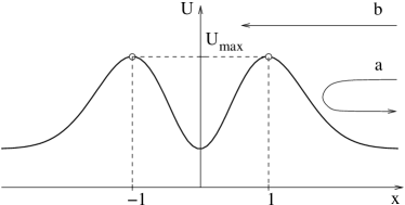
Figure 2: The effective potential for the motion in the adiabatic regime. The particle is reflected at $E<U_{max}$ (case a), and is transmitted through the waveguide at $E>U_{max}$ (case b).

Any particle coming from the right with $E<U_{max}$ gets reflected back; so, these values of $E$, $N$ belong to the classically allowed region. In the opposite case $E>U_{max}$ the particle overcomes the effective potential which means that the reflection process is classically forbidden. Thus, the line $E=N\sqrt{1+a_{0}^{2}{\rm e}^{-1}}$ is the boundary of the classically allowed region at $E,N\ll 1$.

When the values of the parameters $E$, $N$ approach the boundary of the classically allowed region the particle spends more and more time around the tops of the effective barrier $U(x)$. For the values precisely at this boundary there are two unstable solutions $x=\pm 1$. In the two-dimensional picture these solutions correspond to periodic oscillations around the fixed points $(x=\pm 1,y=a_{0}{\rm e}^{-1/2})$ on the axis of the waveguide. We will see that such unstable periodic solutions exist beyond the adiabatic approximation and play a key role in the semiclassical analysis, cf. Refs. Onishi2003 ; Bezrukov:2003yf ; Takahashi2003 . Borrowing the terminology from gauge theories Klinkhamer:1984di we call them excited sphalerons. The sphaleron living at $x\approx 1$ ($x\approx-1$) will be referred to as near (far) sphaleron according to its position relative to the right end of the waveguide.

To identify the boundary of the classically allowed region beyond the adiabatic regime one resorts to numerical methods. We scan through the range of initial phases $0\leq\phi_{0}\leq 2\pi$ at fixed $E$, $N$ and look for the reflected trajectories. If such a trajectory is found at some $\phi_{0}$, the point $(E,N)$ is identified as belonging to the classically allowed region. Otherwise the point is attributed to the classically forbidden domain. The results of these calculations are presented in Fig.3.

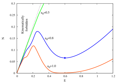
Figure 3: The boundaries $N_{b}(E)$ of the classically allowed regions plotted for $a_{0}=0.5;\,0.8;\,1.0$. The classical reflections are forbidden at $N<N_{b}(E)$. The points to the left of the dashed line $E=N$ correspond to the kinematically forbidden initial conditions.

The boundaries $N_{b}(E)$ of the classically allowed region are obtained for three different values of the parameter $a_{0}$. The classical reflections are allowed for the initial data above the boundaries, $N>N_{b}(E)$, and forbidden below them, $N<N_{b}(E)$. One observes that beyond the adiabatic regime the form of the boundary $N_{b}(E)$ depends qualitatively on the value of $a_{0}$. At small $a_{0}$ it monotonically increases. At $a_{0}\approx 0.5$ a dip in the curve $N_{b}(E)$ develops around $E\approx 0.6$. As $a_{0}$ grows further, this dip becomes lower and more pronounced, until it touches the line $N=0$ at $a_{0}\approx 1$. At even larger values of $a_{0}$ the boundary of the classically allowed region splits into two disconnected parts and a range of energies around $E=0.6$ appears, where the classical reflections are allowed even for $N=0$.

Heuristically, one may envision that the form of the curve $N_{b}(E)$ reflects the behavior of the suppression exponent $F(E,N)$ in the classically forbidden region. Indeed, the suppression exponent is zero above the line $N=N_{b}(E)$. As the value of $N$ gets decreased at fixed energy $E$, the function $F(E,N)$ starts growing at $N=N_{b}(E)$. Thus, the deeper the point is in the classically forbidden domain, the larger is $F$, and vice versa. According to this reasoning the dip in the curve $N_{b}(E)$ at $a_{0}>0.5$ implies that classically forbidden reflection are least suppressed at energies $E\approx 0.6$. Moreover, at $a_{0}<1$ there is a finite range of occupation numbers, $0<N<N_{b}(E=0.6)$, where the reflection process is suppressed at all energies (except for the narrow band $N<E<N\sqrt{1+a_{0}^{2}{\rm e}^{-1}}$ corresponding to the adiabatic regime). For these values of $N$, the suppression exponent $F$ considered as function of $E$ is expected to have a (local) minimum in the vicinity of $E=0.6$. One of the purposes of this paper is to test the method of complex trajectories in the regime when the minimum of $F(E)$ exists; so, we concentrate on the case $a_{0}=0.8$.

Now, we are in a position to investigate the classical dynamics of the system (11) in detail. The observations we make below are crucial for the subsequent study of the classically forbidden reflections. One asks the following question. At given $E,N$ belonging to the classically allowed region, there is a non-empty set ${\cal R}_{E,N}$ of initial phases $\phi_{0}$, which give rise to classical reflections. What is the structure of this set? To answer this question, we fix the initial conditions (12), (14) at $t_{i}=0$ and integrate the equations of motion until $t_{f}=200$ starting from different values of the initial phase $\phi_{0}$. In this way, the dependence of $x_{f}\equiv x(t_{f})$ on $\phi_{0}$ is obtained, see Fig. 4.

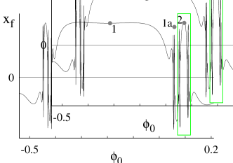
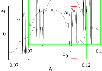
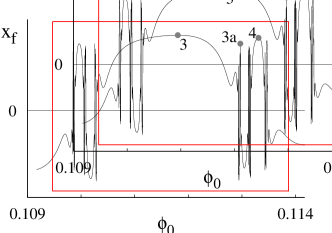
Figure 4: The dependence of the final particle position on the value of the initial phase $\phi_{0}$ for $E=0.6$, $N=0.1$ ($x_{f}$ axis is not to scale). From top to bottom: scaling of the fine structures of the function $x_{f}(\phi_{0})$ reveals self-similar behavior. The corresponding regions in different graphs are marked by the boxes of the same color. The trajectories corresponding to the marked points are shown in Fig. 5.

The negative values of $x_{f}$ correspond to the classical transmissions through the waveguide, while $x_{f}>0$ represent reflections. Thus,

$${\cal R}_{E,N}=\{\phi_{0}|x_{f}(\phi_{0})>0\}\;.$$ (18)

Figure 4 shows that the set ${\cal R}_{E,N}$ is not connected: the intervals of phases corresponding to the reflected trajectories are intermixed with those representing transmissions. Moreover, the scaling of the fine structures of the function $x_{f}(\phi_{0})$ reveals self-similar behavior. One concludes that the set ${\cal R}_{E,N}$ consists of an infinite number of disconnected domains forming a fractal structure. Such a complexity is a manifestation of irregular dynamics inherent in our model; this feature is in sharp contrast to the situation one observes in completely regular systems (see, e.g., the model of Ref. Bonini:1999kj where the analogous set consists of a single interval Bezrukov:2003yf ).

To analyze the nature of irregular dynamics, we consider the trajectories generated by the initial phases which span various connected intervals ${\cal R}_{\alpha;\,E,N}\subset{\cal R}_{E,N}$. All the classical trajectories from a given interval of phases display the same qualitative properties; some features change discontinuously, however, as one goes to another interval. Let us characterize each trajectory by its behavior in the interaction region. To start with, one can distinguish a subset of intervals ${\cal R}_{j;\,E,N}\subset{\cal R}_{E,N}$ corresponding to the trajectories which reach the far sphaleron, perform several oscillations there, and go out of the interaction region back to $x\to+\infty$. We call this subset “the main sequence”. The $x(t)$-dependence for the first four trajectories from the main sequence is plotted in Fig. 5a, while the corresponding values of the initial phase are marked in Fig. 4 by numbers (1 to 4).

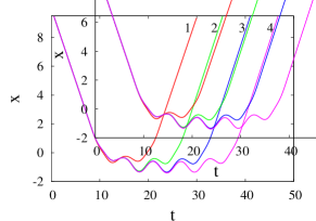
(a)

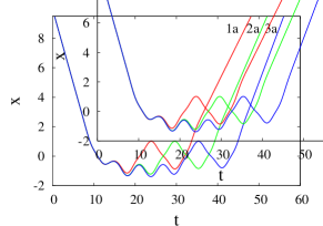
(b)

Figure 5: The main (a) and secondary (b) sequences of trajectories for $E=0.6$, $N=0.1$. The trajectories correspond to initial phases with the same marks as in Fig.4.

Let us make the important observation: all the plotted solutions leave the far sphaleron with approximately the same oscillatory phase. In fact, we have found that this is true for any reflected trajectory. Here lies the root of the disconnectedness of ${\cal R}_{E,N}$: one cannot transform one reflected trajectory into another with a different number of oscillations at the far sphaleron by continuously changing the initial phase. For a solution from the main sequence the index $j$ is equal to the number of oscillations at $x\approx-1$.

The trajectories corresponding to the intervals of ${\cal R}_{E,N}$ other than those from the main sequence display more involved behavior. After oscillating at the far sphaleron they move to the near sphaleron, oscillate an integer number of periods on top of it, return to the far sphaleron, oscillate there once again, etc. As an example we present several trajectories from the next-to-the-main sequence (with only one return to the far sphaleron) in Fig. 5b, they correspond to the initial phases marked by 1a to 3a in Fig. 4. We observed that the motion back and forth between the sphalerons can be arbitrarily complicated giving rise to the aforementioned fractal structure of ${\cal R}_{E,N}$.

For the semiclassical analysis of the next Section it is important to know what happens with the classical reflected solution when the initial phase $\phi_{0}$ approaches the end-point $\phi_{end}$ of an interval ${\cal R}_{\alpha;\,E,N}\subset{\cal R}_{E,N}$. Figure 4 implies that at the ends of the interval the corresponding trajectory gets stuck in the interaction region. More precisely, one observes that as the value of $\phi_{0}$ approaches $\phi_{end}$, the classical solution spends more and more time at $x\approx 1$ before going away to infinity (see Fig. 6), so that

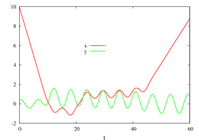
Figure 6: The classical trajectory with the value of the initial phase $\phi_{0}=-0.414$ close to the end–point, $\phi_{0}-\phi_{end}\sim 10^{-3}$, of the first interval of the main sequence; $E=0.6$, $N=0.1$. Before leaving the interaction region the trajectory gets stuck at the near sphaleron for a long time.

the initial datum $\phi_{0}=\phi_{end}$ gives rise to a trajectory which is neither reflected, nor transmitted, but ends up at the near sphaleron. Such a trajectory is unstable: there exist arbitrarily small perturbations which push it out of the interaction region to either end of the waveguide. As the number of intervals (and hence of their end-points) constituting ${\cal R}_{E,N}$ is infinite, the number of the above unstable trajectories is infinite, too. We will see in the next Section that the above unstable solutions give rise to the tunneling trajectories; thus, the classically forbidden reflection process of the next Section provides a particular example of chaotic tunneling.

More insight into the classical dynamics is gained by extending the previous analysis to include the variation of two initial conditions, $\phi_{0}$ and $N$, at fixed energy $E$. One is again interested in the structure of the set ${\cal R}_{E}$ of initial data $(\phi_{0},N)$ which correspond to classical reflections. This set is shown in Fig. 7 ($E=0.6$).

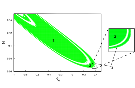
Figure 7: The set ${\cal R}_{E}$ of initial data leading to reflections at $E=0.6$ is painted in green. The inset shows the fine structure near the boundary of ${\cal R}_{E}$. Three first domains of the main sequence are marked by numbers.

As before, it consists of an infinite number of disconnected domains ${\cal R}_{\alpha;\,E}$. Each of these domains is characterized by the way in which the corresponding trajectories travel back and forth between the sphalerons. The domains of the main sequence with $j=1,2,3$ are clearly visible in Fig. 7 along with the secondary ones which accompany them. Figure 7 enables one to understand what happens with the classical reflected trajectories when the occupation number $N$ approaches the boundary of the classically allowed region from above, $N\to N_{b}(E)$; this corresponds to moving to the lower boundary of the set ${\cal R}_{E}$,

$$N_{b}(E)=\inf_{(\phi_{0},N)\in{\cal R}_{E}}N\;.$$

One notices that no matter how close $N$ is to this boundary, the line $N=const$ always has intersections with some domains from the main sequence. In other words, the boundary of the classically allowed region is the accumulation point of the main sequence of domains. On the other hand, as $N$ tends to $N_{b}(E)$, the intersection of the line $N=const$ with certain domains of ${\cal R}_{E}$ disappears. This means disappearance of certain types of trajectories at $N\to N_{b}(E)$. Concentrating on the main sequence, one observes that the remaining trajectories are those with large indices $j$. As the latter are equal to the number of oscillations at the far sphaleron, one concludes that the closer the point $(E,N)$ is to the boundary of the classically allowed region, the longer the corresponding trajectories get stuck at the far sphaleron.

We conclude this section with remarks on the implications of the above classical picture for the semiclassical description of tunneling. It will be shown in Sec. IV that each isolated domain of the set ${\cal R}_{E}$ continues into a branch of tunneling trajectories. Thus, the number of tunneling solutions at given $E$, $N<N_{b}(E)$ is infinite; each of these solutions is associated with a certain domain ${\cal R}_{\alpha;\,E}$. In particular, the fractal structure of ${\cal R}_{E}$ is inherited by the collection of tunneling paths. The above property is very different from that of the models with completely regular classical dynamics Bezrukov:2003yf where the tunneling solution is unique. On the other hand, an infinite number of tunneling trajectories seems to be generically inherent in chaotic systems Shudo1995_1 . According to the general rules, the suppression exponent $F$ in Eq. (1) is equal to the lower bound of the suppressions calculated on all the tunneling solutions,

$$F(E,N)=\inf_{\alpha}F_{\alpha}(E,N)\;,$$ (19)

where the index $\alpha$ marks the solutions. At first glance it is not clear how the lower bound (19) can be found: one is unable to compute the suppression exponents of an infinite set of trajectories. Two observations which greatly simplify the problem are as follows. First, it will be shown below that the nearer the domain ${\cal R}_{\alpha;\,E}$ is to the boundary of the classically allowed region, the smaller is the suppression exponent of the tunneling solution associated with it. Second, the domains of the main sequence accumulate near the boundary of the classically allowed region. This implies that the suppression exponents $F_{j}$ of the tunneling trajectories from the main sequence decrease with the index $j$. Moreover, for any tunneling path there exist tunneling solutions from the main sequence with the same $E$, $N$ and smaller value of the suppression exponent. Thus, in order to calculate the lower bound (19) it is sufficient to consider the trajectories from the main sequence, compute their suppression exponents $F_{j}$, and take the limit,

$$F(E,N)=\lim_{j\to\infty}F_{j}(E,N)\;.$$ (20)

This tactics is implemented in the next section.

IV Semiclassical study

We now formulate the boundary value problem for the tunneling trajectories. The probability (8) of over-barrier reflection is described by the complexified solution to the classical equations of motion

$$\frac{\delta S}{\delta x(t)}=\frac{\delta S}{\delta y(t)}=0$$ (21a)

obeying the following boundary conditions,

$$\frac{{\dot{x}}^{2}}{2}+N=E~{},~{}~{}~{}\frac{{\dot{y}}^{2}}{2}+\frac{y^{2}}{2}=N, \mathrm{at}~{}~{}~{}~{}~{}t\to-\infty\;,$$ (21b)

$$\mathop{\rm Im}\nolimits x~{},~{}~{}\mathop{\rm Im}\nolimits y\to 0, \mathrm{at}~{}~{}~{}~{}~{}t\to+\infty\;.$$ (21c)

Here $E$, $N$ stand for the (rescaled, see Eqs. (13)) energy and initial occupation number. The initial conditions (21b) at $t\to-\infty$ can be cast into the form (12b), (14), where the initial phase $\phi_{0}$ is now allowed to take complex values. Similarly, $x(t_{i})$ is also complex, in general. The boundary conditions (21b), (21c) have clear physical interpretation. Equations (21b) fix the quantum numbers ${\cal E}$, ${\cal N}$ of the initial quantum state. Due to the uncertainty principle this makes the two conjugate coordinates, $\phi_{0}$ and $x(t_{i})$, maximally indeterminate. Accordingly, in the semiclassical picture they become complex–valued. On the other hand, the quantum numbers of the final states are not fixed, and Eqs. (21c) imply that the particle comes out in a classical state with real coordinates and momenta.

Note that, generically, the tunneling solution is defined along a certain contour in the complex time plane. In our case, however, the contour is trivial: it runs along the real time-axis.

It is useful to parametrize the imaginary parts of $x(t_{i})$ and $\phi_{0}$ as follows,

$$2\mathop{\rm Im}\nolimits x(t_{i})=-\dot{x}(t_{i})T\;,$$ (22)

$$2\mathop{\rm Im}\nolimits\phi_{0}=-T-\theta\;,$$ (23)

where $T$ and $\theta$ are real parameters. Then the suppression exponent of a given complex trajectory is

$$F_{\alpha}=2\mathop{\rm Im}\nolimits\tilde{S}_{\alpha}-ET_{\alpha}-N\theta_{\alpha}\;,$$ (24)

where the two last terms result from the non–trivial initial state of the process, while

$$\tilde{S}_{\alpha}=\frac{1}{2}\int dt\left(-x\ddot{x}-y\ddot{y}-(y-a(x))^{2}\right)$$ (25)

is the classical action integrated by parts. The subscript $\alpha$ is introduced to remind that there may exist several tunneling solutions with given $E$, $N$.

We do not present the derivation of the above boundary value problem. The logic is completely analogous to that of Refs. Bonini:1999kj ; Bezrukov:2003yf ; prefactor ; wigles , and an interested reader is referred to these papers. The field theory analog of the problem (21) was first introduced in Ref. Rubakov:1992ec .

It is important to remark that the problem (21) does not guarantee per se that its solutions describe reflections. To ensure that this is the case, one supplements Eqs. (21) with the condition

$$\mathop{\rm Re}\nolimits x\to+\infty~{}~{}~{}~{}~{}~{}~{}\mathrm{at}~{}~{}~{}t\to+\infty\;.$$ (26)

Below we find solutions which satisfy this requirement by using the $\epsilon$–regularization method of Refs. Bezrukov:2003yf .

Let us explain the physical meaning of the initial-state parameters $T$, $\theta$. One can prove the relations (see, e.g., Refs. Bezrukov:2003yf ; wigles )

$$T=-\frac{\partial}{\partial E}F(E,N)\;,\qquad\qquad\theta=-\frac{\partial}{\partial N}F(E,N)\;,$$ (27)

which imply that $T$ and $\theta$ are the derivatives of the suppression exponent with respect to energy and initial oscillator excitation number. One notices that $T$, $\theta$ can be used instead of $E$, $N$ to parametrize the tunneling paths. Then, the solutions with $T=0$ correspond to the extrema of the suppression exponent with respect to energy. These solutions are called “real–time instantons”, they can be found directly using the method of Ref. Levkov:2004tf . Calculating the value of the functional (24) on them, one obtains the extremal (notably, minimal) values of the suppression exponent at $N=const$. The method of real–time instantons is important in field theory Levkov:2004tf , where it enables one to calculate the minimal suppression of the collision–induced tunneling. One of the purposes of this paper is to check the above method by the explicit comparison with the exact quantum mechanical results. Accordingly, we pay specific attention to the region around the minimum of the suppression exponent $F(E)$.

We solve the boundary value problem (21) numerically with the deformation procedure. Namely, the solution with energy $E+\Delta E$ and oscillator excitation number $N+\Delta N$ is found by the iterative Newton–Raphson method NumericalRecipes starting from the solution at $E$, $N$, which serves as the zeroth–order approximation. In this way, an entire branch of tunneling trajectories can be obtained starting from a single solution and walking in small steps in $E$, $N$. The details of our numerical technique can be found in Refs. Bonini:1999kj , see Refs. Kuznetsov:1997az ; Bezrukov:2003er for the applications in field theory.

The only non-trivial task of the above approach is to find the input for the first deformation. The idea we put forward in this paper is to start the procedure from the classically allowed region and arrive at the tunneling solutions by changing the values of $E$, $N$ in small steps. [Note that the approach of obtaining complex trajectories from the real ones was also implemented in a different context in Ref.Xavier1996 .] One begins with the observation that the real classical trajectories satisfy Eqs. (21). Naively, one takes a trajectory with $E$, $N$ from the classically allowed region, and decreases the value of $N$ with the hope to get the correct tunneling solution at $N<N_{b}(E)$. However, serious obstacles arise on the way. First, the classical solution is not unique at given $E$, $N$; the degeneracy is parametrized by the initial phase $\phi_{0}\in{\cal R}_{E,N}$. This makes the numerical implementation of the deformation procedure problematic. Second, suppose one takes the initial data $(N,\phi_{0})$ belonging to some connected domain ${\cal R}_{\alpha;\,E}\subset{\cal R}_{E}$ and decreases $N$. It was observed in Sec. III that, as the value of $N$ approaches the boundary $N=N_{b,\alpha}(E)$ of ${\cal R}_{\alpha;\,E}$ from above, the reflected classical solution spends more and more time in the interaction region. At $N=N_{b,\alpha}(E)$ it gets stuck at $x\approx 1$ forever, merging at this point with the classical solutions, which represent the transmissions of the particle through the waveguide at $N<N_{b,\alpha}(E)$. Here lies the worst obstruction: the transmitted classical trajectories obviously solve the boundary value problem (21), so that the deformation procedure which starts from the classically allowed region will produce them at $N<N_{b,\alpha}$, instead of the correct complex reflected solutions. One concludes that the condition (26) should be somehow incorporated explicitly into the boundary value problem.

A method which automatically fixes the asymptotic (26) of the solution is proposed in Refs. Bezrukov:2003yf ; prefactor . It is called $\epsilon$–regularization. Here we briefly describe this method concentrating on its application to the problem at hand. A more detailed description of the technique can be found in Refs. Bezrukov:2003yf ; prefactor . One replaces the action of the system in Eqs. (21), (24) with the modified action

$$S_{\epsilon}[{\boldsymbol{x}}]=S[{\boldsymbol{x}}]+i\epsilon T_{int}[{\boldsymbol{x}}]\;.$$ (28)

Here $\epsilon$ is small and positive, while the functional $T_{int}$ measures the time the particle spends in the interaction region. The simplest choice is

$$T_{int}=\int dtf(x(t),y(t))\;,$$ (29)

where the function $f$ is real and positive at $x,\,y\in{\mathbb{R}}$, and is localized in the interaction region. Otherwise the choice of $f$ is arbitrary: the final result is recovered in the limit $\epsilon\to+0$ and does not depend on the particular form of this function. We use

$$f=\tilde{\theta}(1-x)\tilde{\theta}(x-1)\;,$$ (30)

where

$$\tilde{\theta}(x)=\frac{1}{1+{\rm e}^{-2x-x^{3}}}$$ (31)

is the smeared $\theta$–function. Note that $f$ peaks at the near sphaleron; this choice will be explained shortly.

One notices two important changes that the substitution (28) brings into the boundary value problem (21). First, the degeneracy of the classical solutions is removed at $\epsilon\neq 0$. Indeed, any unperturbed classical trajectory extremizes the original action functional $S[{{\boldsymbol{x}}}]$, so that at fixed $E$, $N$ and $\epsilon=0$ there exists a valley of extrema parametrized by $\phi_{0}$. The functional $T_{int}[{\boldsymbol{x}}]$, however, discriminates among all these extrema and lifts the valley. Correspondingly, at small $\epsilon>0$ the extrema of the regularized action $S_{\epsilon}[{\boldsymbol{x}}]$ are close to the classical reflected solutions with $\partial T_{int}/\partial\phi_{0}=0$ (see Refs. Bezrukov:2003yf for the detailed discussion). From the physical viewpoint this can be understood as follows. In the $\epsilon$–regularized case the suppression, Eq. (24), of the trajectories in the classically allowed region is not precisely zero because of the complex term $i\epsilon T_{int}$ in Eq. (28). The suppression is minimized on the real classical trajectories corresponding to the minima of $T_{int}$; therefore, the solutions to Eqs. (21), (28), which by construction correspond to the least suppressed reflections, are close to the above classical trajectories.

In practice, one starts with the function $T_{int}(\phi_{0})$ representing the values of $T_{int}$ on the classical trajectories with fixed $E$, $N$ and $\epsilon=0$, finds the extrema of this function, and uses the corresponding trajectories as the zeroth–order approximation to the solutions of Eqs. (21), (28) with small, but non-zero $\epsilon$.

The second useful property of the $\epsilon$–regularization comes about as one tries to decrease the value of the initial oscillator excitation number, and cross the boundary $N=N_{b,\alpha}(E)$ of a given classically allowed domain. One discovers that at $\epsilon\neq 0$ each reflected trajectory at $N>N_{b,\alpha}(E)$ is smoothly connected with the complex reflected solution at $N<N_{b,\alpha}(E)$. The reason, again, lies in the additional suppression caused by the term $i\epsilon T_{int}$ in the action. Although the reflected trajectories get only slightly perturbed at small $\epsilon$, the solutions ending up in the interaction region at $t\to+\infty$ change drastically. Indeed, the functional $T_{int}[{\boldsymbol{x}}]$ diverges on the latter trajectories giving rise to the infinite suppression. The immediate consequence is that the paths which get stuck in the interaction region are excluded from the set of solutions to the boundary value problem (21), (28). Now, the solutions to Eqs. (21), (28) cannot change their asymptotic (26): starting from the classical reflected solution and decreasing the value of the initial excitation number $N$ in small steps, one leaves the classically allowed region and obtains the correct complex reflected trajectories.

Let us briefly comment on the choice of the contour in the complex time plane which carries the tunneling solutions. Obviously, the classical trajectories, which are the starting point of our deformation procedure, run along the real time axis. Generically, while moving into the classically forbidden region, one may need to deform the time contour in order to avoid the singularities of the solution, see Refs. Bezrukov:2003yf . In the actual calculations of this paper we did not encounter such a necessity. The time contour was always kept coincident with the real axis.

An example of a regularized tunneling solution deep inside the classically forbidden region ($E=0.6$, $N=0$) is shown in Fig. 8b.

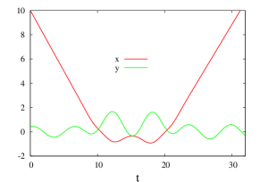
(a)

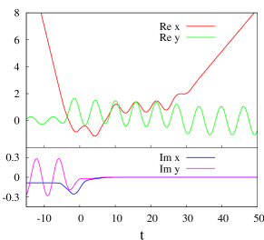
(b)

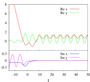
(c)

Figure 8: (a) The reflected classical trajectory from the first domain of the main sequence, corresponding to the minimum of $T_{int}(\phi_{0})$ ($E=0.6$; $N=0.1$; $\phi_{0}=-0.366$). (b) The regularized tunneling solution ($E=0.6$, $N=0$, $\epsilon=10^{-6}$) descended from the above classical trajectory. (c) The limit $\epsilon\to 0$ of the tunneling solution.

The depicted solution descends from the classical reflected trajectory with $E=0.6$, $N=0.1$, $\phi_{0}=-0.366$ (see Fig. 8a), which (locally) minimizes the function $T_{int}(\phi_{0})$; the regularization $\epsilon=10^{-6}$ was switched on and $N$ was gradually decreased by small steps. Note that the solution in Fig. 8b is genuinely complex and satisfies the requirement (26).

The solutions to the original boundary value problem are recovered in the limit $\epsilon\to+0$; the suppression exponents of the unperturbed trajectories are

$$F_{\alpha}(E,N)=\lim_{\epsilon\to+0}F_{\alpha,\epsilon}(E,N)\;.$$ (32)

Practically, the removal of the regularization is carried out by taking $\epsilon$ to be small enough, $\epsilon\mathchoice{\mathrel{\vbox{\hbox{$\buildrel\displaystyle<\over{\displaystyle\sim}$}}}}{\mathrel{\vbox{\hbox{$\buildrel\textstyle<\over{\textstyle\sim}$}}}}{\mathrel{\vbox{\hbox{$\buildrel\scriptstyle<\over{\scriptstyle\sim}$}}}}{\mathrel{\vbox{\hbox{$\buildrel\scriptscriptstyle<\over{\scriptscriptstyle\sim}$}}}}10^{-6}$. At these $\epsilon$, the values of the suppression exponents $F_{\alpha,\epsilon}$ stabilize at the level of accuracy $O(10^{-5})$ which is sufficient for our purposes.

As one tries to take the limit $\epsilon\to+0$ of the tunneling trajectory itself, a surprise comes about. Namely, as $\epsilon$ gets decreased, the regularized tunneling trajectories deep inside the classically forbidden region stay longer and longer at finite $x$, so that the trajectories with $\epsilon=0$ do not escape to infinity, but end up on an unstable solution – the near sphaleron – living at $x\approx 1$. [An example of unperturbed tunneling trajectory ($E=0.6$, $N=0$, $\epsilon=0$) is shown in Fig. 8c.] Strictly speaking, the solutions at $\epsilon=0$ do not describe reflection, but rather creation of the unstable state, the sphaleron. Nevertheless, their suppression exponents are relevant for tunneling as the latter state decays into the asymptotic region $x\to+\infty$ without exponential suppression. The mechanism of dynamical tunneling via creation of unstable periodic orbits was discovered independently in Refs. Bezrukov:2003yf and Refs. Takahashi2003 .

We remark that all unregularized tunneling trajectories in the model under consideration tend to the unstable sphaleron solution at $t\to+\infty$, and thus turn out to be unstable themselves. Straightforward numerical methods are inappropriate for finding such trajectories Bonini:1999kj , while $\epsilon$–regularization provides a universal method for treating such instabilities.

Let us now discuss the structure of tunneling solutions. Following the above strategy, one starts with the classical reflected solutions. It is straightforward to see that the function $T_{int}(\phi_{0})$ has at least one extremum in every connected interval ${\cal R}_{\alpha;\,E,N}$ in the set of reflection phases ${\cal R}_{E,N}$. Indeed, the classical reflected trajectories with $\phi_{0}\in{\cal R}_{\alpha;\,E,N}$ spend finite time in the interaction region and smoothly depend on the initial data, producing the smooth function $T_{int}(\phi_{0})$. On the other hand, the classical trajectories spend more and more time at the near sphaleron as $\phi_{0}$ approaches the end-points of ${\cal R}_{\alpha;\,E,N}$ (see Sec. III). Thus, $T_{int}(\phi_{0})$ tends to infinity at the end points of this interval, necessarily attaining a minimum somewhere in between. [Note that the specific form of the functional $T_{int}$ (function $f$ in Eq. (29) peaks at $x\approx 1$) has been chosen in accordance with the tendency of classical trajectories to get stuck at the near sphaleron.] Thus, starting from each interval ${\cal R}_{\alpha;\,E,N}$, one obtains one branch of solutions to the $\epsilon$-regularized problem. Note that, as ${\cal R}_{E,N}$ is the section of the set ${\cal R}_{E}$ by the line $N=const$, the domains of ${\cal R}_{E}$ may correspond to two disconnected intervals of ${\cal R}_{E,N}$, see Fig. 7. When $N$ gets decreased, these intervals merge. Below we assume that the starting classical solution of the type $\alpha$ has been taken at small enough $N$, such that the domain ${\cal R}_{\alpha;\,E}$ gives rise to a single interval of phases ${\cal R}_{\alpha;\,E,N}$. Then, the fractal structure of ${\cal R}_{E}$ is inherited by the complex tunneling paths: the distinct branches of complex trajectories are in one–to–one correspondence with the connected domains of the set ${\cal R}_{E}$.

Now, we can give a heuristic justification of the claim made in the end of Sec. III: the nearer the domain ${\cal R}_{\alpha;\,E}\subset{\cal R}_{E}$ lies to the boundary of the classically forbidden region, the less suppressed is the corresponding tunneling trajectory. Let us consider two branches of solutions stemming from the domains 1 and 2 in Fig. 7. The line $N=0.07$ intersects with the domain 2, so that the point $E=0.6$, $N=0.07$ belongs to the classically allowed region, and the suppression of the solution 2 vanishes in the limit $\epsilon\to 0$. On the other hand, the line $N=0.07$ does not cross the domain 1. Thus, at $E=0.6$, $N=0.07$ the corresponding solution to Eqs. (21), (28) is genuinely complex and has non-zero suppression even at $\epsilon\to 0$. Suppose that one decreases $N$ and enters the classically forbidden region. At some point the solution of the type 2 also becomes classically forbidden. It is clear that at least for some range of $N$, its suppression remains weaker than that of the solution 1. This suggests, though does not guarantee, the same hierarchy of suppressions inside the entire classically forbidden region. Below, we check the conjectured hierarchy explicitly.

Let us discuss in detail the case $N=0$ (no transverse oscillations in the initial state) corresponding to the extreme values of parameters inside the forbidden region; all the qualitative features are the same for other values of $N$ as well. Our strategy is to find the limit (20) of the main sequence of suppressions $F_{j}$, and check that this limit represents the lower bound of the suppression exponents of all the tunneling solutions.

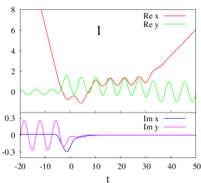
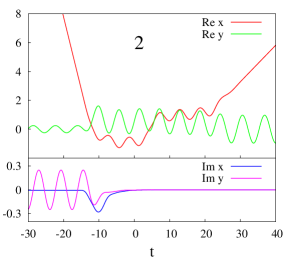
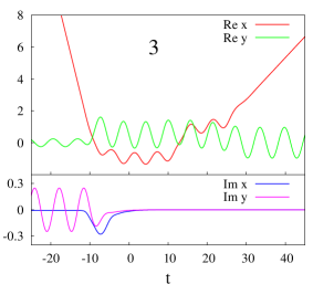
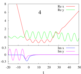
Figure 9: Four tunneling solutions from the main sequence; $E=0.5$, $N=0$, $\epsilon=10^{-6}$.

Figure 9 shows several first representatives of the main sequence of tunneling paths at $E=0.5$, $N=0$, $\epsilon=10^{-6}$. Similar to their classical progenitors, the branches of tunneling trajectories may be classified according to the number of oscillations they perform at the far sphaleron. On the contrary, the number of oscillations at the near sphaleron is not an invariant of the branch: as discussed above, it grows as the regularization parameter $\epsilon$ gets decreased, so that the tunneling trajectories get stuck at the near sphaleron at $\epsilon=0$. Another important observation about the plots in Fig. 9 is that the imaginary parts of the solutions are sizeable only in the beginning of the evolution. They fall off rapidly during the oscillations at the far sphaleron and become small at late times. This qualitative feature holds for the trajectories at other energies as well. Thus, the suppression exponents of the trajectories are saturated during the first few oscillations at the far sphaleron, and depend weakly on the subsequent evolution. In addition, the trajectories from the main sequence almost coincide in the beginning of the process.

$j\,\diagdown\,E$	0.1	0.3	0.5	0.7	0.9
1	0.3188	0.1625	0.1098	0.1398	0.2259
2	0.2586	0.1380	0.0991	0.1341	0.2221
3	0.2373	0.1340	0.0979	0.1336	0.2219
4	0.2307	0.1333	0.0978	0.1336	0.2219
5	0.2285	0.1331	0.0978	0.1336	0.2219
$\infty$	0.2272	0.1331	0.0978	0.1336	0.2219

Table 1: The suppression exponents of the complex trajectories from the main sequence at $N=0$. The rows represent the indices $j$ of the trajectories, while the columns correspond to the values of energy $E$. The last row refers to the limiting solution.

This implies fast convergence of the suppression exponents $F_{j}$ to the limiting value $F$ according to the formula (20).

The above convergence is demonstrated in Table 1, where the suppression exponents $F_{j}(E)$ are presented for several values of energy $E$ at $N=0$. As expected from the heuristic argument, the value of $F_{j}$ decreases as $j$ gets larger. The limiting values $F(E)$ are also included into Table 1.

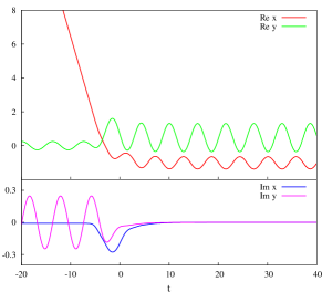
Figure 10: The limit of the main sequence of tunneling trajectories: the solution which gets stuck at the far sphaleron; $E=0.5$, $N=0$.

They can be obtained by extrapolating the dependences of the suppression exponents $F_{j}$ on $j$, which are well fitted by the formula

$$F_{j}=F+a{\rm e}^{-bj}\;,$$

where $a$, $b$ are real positive coefficients. A better way, which is exploited in this paper, is to find the limit $j\to+\infty$ of the tunneling solution itself, and then calculate the limiting value of the suppression exponent using Eq. (24). The limiting solution performs an infinite number of oscillations on the far sphaleron; it can be obtained numerically by the method described in App. A. The limiting solution at $E=0.5$, $N=0$ is shown in Fig. 10.

So far we have considered only the tunneling trajectories from the main sequence and demonstrated that Eq. (20) reproduces the lower bound of their suppressions.

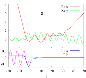
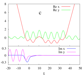
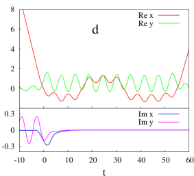
Figure 11: The examples of secondary tunneling trajectories; $E=0.5$, $N=0$, $\epsilon=10^{-6}$.

We have checked that the limiting value $F(E)$ is lower than the suppression exponents of other tunneling trajectories as well. As an illustration, consider the tunneling trajectories shown in Fig. 11. The differences between their suppression exponents and that of the limiting solution are plotted in Fig. 12.

Figure 12: The difference between the suppression exponents of the secondary trajectories of the types shown in Fig. 11 and that of the limiting solution; $N=0$.

The limiting solution is evidently the least suppressed one.

Let us discuss the physical interpretation of the obtained results. The form of the limiting solution implies that the reflection process in our model proceeds in two stages. First, the far sphaleron state gets created. This stage is exponentially suppressed due to the essential modification of the particle state needed for the sphaleron creation. Second, the sphaleron state decays into the asymptotic region $x\to+\infty$ with probability of order $1$. This two-stage process is a manifestation of the phenomenon of “tunneling on top of the barrier” Takahashi2003 ; Bezrukov:2003yf ; the phenomenon is generic for the inclusive tunneling processes, see Refs. Bezrukov:2003er ; Levkov:2004tf for the field theoretical examples.

Remarkably, though we came to the limiting solution considering the accumulation point of an infinite number of complicated tunneling paths, the solution itself is unique and very simple. All the chaotic features of motion, like going back and forth between the sphalerons, are related to the second stage of the reflection process: the decay of the far sphaleron. As the second stage is unsuppressed, one might conclude that, after all, the chaotic motions are irrelevant for the calculation of the main suppression exponent. Note, however, that one is not able to guess from the beginning, which tunneling solution corresponds to the smallest suppression; therefore, the systematic analysis of the chaotic motions is essential. Besides, the sub-dominant contributions of the chaotic trajectories might be important for the analysis of the process at finite values of the semiclassical parameter $g$ Adachi:1986 ; Shudo:1996 ; Onishi2003 .

The final semiclassical results for the dependence of the suppression exponent $F$ on energy $E$ for $N=0;\,0.02;\,0.04$ are presented in Fig. 13.

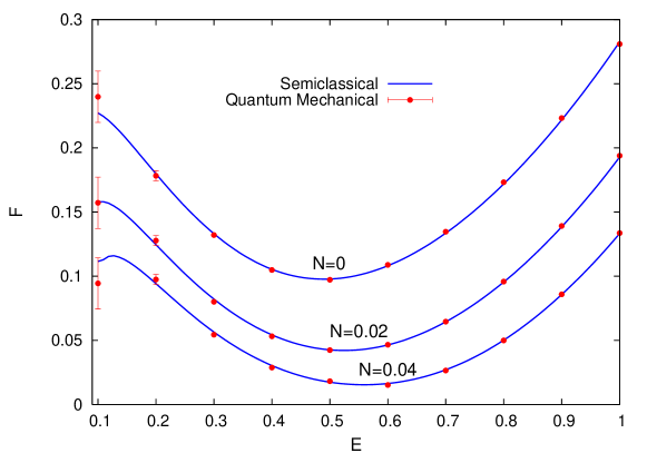
Figure 13: The semiclassical (lines) versus quantum mechanical (points) results for the suppression exponent $F(E)$ at three different values of $N$. The errors of the quantum mechanical computations are smaller than the point size for $E\geq 0.3$.

Note that the suppression exponent is non-monotonic function of energy with the minimum near $E=0.5$. We remind that the minima of $F(E)$ correspond to the particularly interesting solutions, real–time instantons.

V Exact quantum computations

In this Section we extract the suppression exponent $F$ from the exact reflection probability (8). One begins by solving numerically the Schrödinger equation

$${\cal H}|\psi\rangle={\cal E}|\psi\rangle\;.$$ (33)

It is convenient to work in the original variables $X$, $Y$, $P_{X}$, $P_{Y}$, see Eq. (5), in order to bring the kinetic term of the Hamiltonian into the canonical form. One rewrites Eqs. (2), (3) as

$${\cal H}=\frac{P_{X}^{2}+P_{Y}^{2}}{2}+\frac{1}{2}(Y-\tilde{a}(X))^{2}\;,$$ (34)

where

$$\tilde{a}(X)=\frac{1}{g}a(gX)\;.$$ (35)

Basically, our numerical technique follows the lines of Refs. Bonini:1999kj ; Levkov:2002qg . One works in the asymptotic basis formed by a direct product of the translatory coordinate eigenfunctions $|X\rangle$ and eigenfunctions $|n\rangle$ of the $y$–oscillator with the fixed frequency $\omega=1$,

$$\psi_{n}(X)=\langle X,\,n|\psi\rangle\;.$$

The stationary Schrödinger equation (33) reads,

$$\frac{d^{2}}{dX^{2}}\psi_{n}(X)=\sum_{n^{\prime}}A_{nn^{\prime}}(X)\psi_{n^{\prime}}(X)\;,$$ (36)

where

$$A_{nn^{\prime}}(X)=\langle n|\hat{P}_{Y}^{2}+(\hat{Y}-\tilde{a}(X))^{2}-2{\cal E}|n^{\prime}\rangle\\ =\delta_{n,n^{\prime}}(2n+1+\tilde{a}^{2}(X)-2{\cal E})\\ -\tilde{a}(X)(\delta_{n,n^{\prime}-1}\sqrt{2n+2}+\delta_{n,n^{\prime}+1}\sqrt{2n})$$

is an infinite three–diagonal matrix.

In the asymptotic regions $X\to\pm\infty$, $\tilde{a}(X)\to 0$ the interaction terms become negligibly small, and the solution takes the form,

$$\psi_{n}(X)\to r_{n}^{\pm}\mathrm{e}^{iP_{n}X}+t_{n}^{\pm}\mathrm{e}^{-iP_{n}X}\;,$$ (37)

where

$$P_{n}=\sqrt{2{\cal E}-(2n+1)}$$ (38)

stands for the asymptotic translatory momentum of the $n$-th mode. The boundary conditions for the stationary wave function $\psi_{n}(X)$ are constructed in the standard way. The particle comes from the right, $X\to+\infty$, in the ${\cal N}$–th oscillator state; hence, we fix

$$t_{n}^{+}=\delta_{n,{\cal N}}\;.$$ (39)

On the other hand, only the outgoing wave should remain at $X\to-\infty$,

$$r_{n}^{-}=0\;.$$ (40)

Note that while the low–lying modes are oscillatory at the asymptotic, the ones with $n>{\cal E}-1/2$ grow (decay) exponentially, see Eq. (38). Physically, the latter correspond to the kinetically inaccessible region, where the energy of the transverse oscillations exceeds ${\cal E}$. We fix the boundary conditions for them by killing the parts growing exponentially toward infinities. One notes that after the proper continuation of Eq. (38),

$$P_{n}=i\sqrt{(2n+1)-2{\cal E}}\;,\qquad n>{\cal E}-1/2\;,$$ (41)

the aforementioned conditions coincide with Eqs. (39), (40).

Equations (36), (39), (40) constitute the boundary value problem to be solved numerically. After the stationary wave function $\psi_{n}(X)$ is found, one calculates the probability current

$$J=\mathrm{Im}\,\sum_{n}\psi_{n}^{*}(X)\frac{d}{dX}\psi_{n}(X)\;,$$ (42)

and hence the reflection probability

$${\cal P}=\frac{|J^{(\mathrm{out})}|}{|J^{(\mathrm{in})}|}=\sum_{n<{\cal E}-1/2}\frac{P_{n}}{P_{\cal N}}|r_{n}^{+}|^{2}\;,$$ (43)

where the currents $J^{(\mathrm{in})}$ and $J^{(\mathrm{out})}$ are computed with the incoming and outgoing parts of the wave function at $X\to+\infty$, respectively.

The details of the numerical formulation of the problem (36), (39), (40) are presented in App. B. Let us discuss the results.

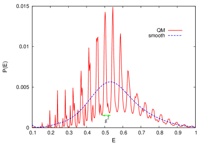
Figure 14: The function ${\cal P}(E)$ plotted for $N=0$, $g=0.2$. The dashed curve represents the smoothened result, Eq. (45).

The typical dependence of the reflection probability ${\cal P}$ on energy $E=g^{2}{\cal E}$ is shown in Fig. 14, solid line (the values of the other parameters are $N\equiv g^{2}{\cal N}=0$, $g=0.2$). The striking feature is that the graph is modulated by sharp oscillations. At first glance, this picture is incompatible with the results of the semiclassical analysis, where we obtained, at least in the leading order, that the tunneling probability, ${\cal P}\propto{\rm e}^{-F(E)/g^{2}}$, is a smooth function of energy. We are going to demonstrate the opposite: the quantum mechanical results reconcile nicely with the semiclassical ones.

By computing the reflection probability at different $g$, one notices the following important properties. First, the period of oscillations scales like $\tau_{E}\propto g^{2}$. So, in the semiclassical limit $g\to 0$ the oscillations become more and more frequent. Second, one considers $F_{g}\equiv g^{2}\mathop{\rm ln}\nolimits{\cal P}$ and asks whether the amplitude of oscillations of this quantity goes to zero in the limit $g\to 0$. We certainly observed that it drops down as $g$ decreases though we were unable to figure out whether it indeed vanishes at $g\to 0$. The properties mentioned above suggest the interpretation of the oscillations as the result of the quantum interference between the contributions of various tunneling trajectories found in Sec. IV. Suppose for simplicity that there are only two such trajectories. Let us denote their complex actions by $S_{1}(E)$ and $S_{2}(E)$ (we omit the dependence on $N$). Then, the total reflection amplitude reads,

$$r\sim A_{1}\mathrm{e}^{iS_{1}(E)/g^{2}}+A_{2}\mathrm{e}^{iS_{2}(E)/g^{2}}\;.$$

For the sake of argument we suppress the index $n$ and disregard the initial–state contributions into the exponents. In the above formula $A_{1}$ and $A_{2}$ stand for the pre-exponential factors of the partial processes. For the reflection probability one writes,

$${\cal P}\propto|r|^{2}\sim|A_{1}|^{2}\mathrm{e}^{-2\mathrm{Im}\,S_{1}(E)/g^{2}}+|A_{2}|^{2}\mathrm{e}^{-2\mathrm{Im}\,S_{2}(E)/g^{2}}\\ +2|A_{1}A_{2}|\mathrm{e}^{-\mathrm{Im}\,(S_{1}(E)+S_{2}(E))/g^{2}}\times\\ \times\cos\left[\mathrm{Re}\,(S_{1}(E)-S_{2}(E))/g^{2}+\mathrm{arg}(A_{1}/A_{2})\right]\;.$$ (44)

Along with the terms corresponding to the probabilities of the partial processes, one gets the interference term, which results in oscillations with period $\tau_{E}$ of order $g^{2}$. Of course, if one of the solutions, say, the first one, is dominant, $\mathrm{Im}\,S_{1}<\mathrm{Im}\,S_{2}$, the relative contributions of the two last terms in Eq. (44) vanish exponentially fast at $g\to 0$. In our case the situation is more subtle, however. As the semiclassical analysis reveals, in the model under consideration there exists an infinite number of tunneling paths, which pile up near the dominant limiting solution. So, at each finite value of $g$ there are solutions which satisfy $\mathrm{Im}\,(S_{2}-S_{1})\lesssim g^{2}$ (the index “$1$” still marks the dominant solution here). Thus, the sum (44) always contains an infinite number of oscillating terms producing a complicated interference pattern; it is not clear whether the oscillations disappear at small $g$.

What saves the day is the aforementioned scaling of the oscillation period. Indeed, $\tau_{E}$ vanishes at $g\to 0$ implying that the oscillations become indiscernible in the semiclassical limit. One obtains a quantity which is well-behaved in this limit by averaging the reflection probability over several periods of oscillations. To be more precise, we consider the smoothened probability

$${\cal P}^{(s)}(E,N)=\int dE^{\prime}\,{\cal D}_{\sigma}(E-E^{\prime}){\cal P}(E^{\prime},N)\;,$$ (45)

where ${\cal D}_{\sigma}$ is the bell-shaped function,

$$D_{\sigma}(E)=\frac{\mathrm{e}^{-E^{2}/\sigma^{2}}}{\sigma\sqrt{\pi}}\;,\qquad\int dE\,D_{\sigma}(E)=1\;.$$

If $\sigma=g^{2}\Sigma$, where $\Sigma$ is a fixed number, the smoothening (45) does not spoil the value of the dominant suppression exponent. Indeed, for the first term in Eq. (44) one writes,

$${\cal P}^{(s,\mathrm{dom})} \propto\int dE^{\prime}\,|A_{1}|^{2}\mathrm{e}^{-F_{1}(E^{\prime})/g^{2}}{\cal D}_{\sigma}(E^{\prime}-E)$$ (46)

$$\approx|A_{1}|^{2}\mathrm{e}^{{F_{1}^{\prime}}^{2}(E)\Sigma^{2}/4}\cdot\mathrm{e}^{-F_{1}(E)/g^{2}}\;,$$

where $F_{1}=2\mathrm{Im}S_{1}$, $F_{1}^{\prime}=dF_{1}/dE$, and we made use of the Taylor series expansion in the second equality. It is clear that only the pre-exponential factor is affected by the integration (45), while the exponent $F_{1}(E)$ is left intact. On the other hand, at large enough values of the coefficient $\Sigma$ the formula (45) represents averaging over many oscillatory periods, which kills all the oscillating contributions. Indeed, consider the typical interference term,

$${\cal P}^{(\mathrm{osc})}\propto C(E)\mathrm{e}^{-F_{0}(E)/g^{2}}\times\\ \times\cos\left[\Delta S(E)/g^{2}-\Delta\phi(E)\right]\;,$$ (47)

where $F_{0}=\mathrm{Im}(S_{1}+S_{2})$, $\Delta S=\mathrm{Re}(S_{1}-S_{2})$, $C=2|A_{1}A_{2}|$, $\Delta\phi=\mathrm{arg}(A_{1}/A_{2})$. Performing integration, one obtains,

$${\cal P}^{(s,\mathrm{osc})}(E)\propto C\mathrm{e}^{-F_{0}/g^{2}}\cos\left[\Delta S/g^{2}+\Delta\phi-F_{0}^{\prime}\Delta S^{\prime}\Sigma^{2}/2\right]\\ \times\exp\left\{\frac{\Sigma^{2}}{4}(F_{0}^{\prime 2}-\Delta S^{\prime 2})\right\}\;.$$

Taking into account that $F_{0}^{\prime}\approx F_{1}^{\prime}$ we see that the interference term is suppressed by the additional factor $\exp\{-\Sigma^{2}\Delta S^{\prime 2}/4\}$ with respect to the dominant contribution (46). Below we fix $\Sigma=1$. We observed that the interference patterns get multiplied by $10^{-3}$ in this case; the latter number is accepted as the precision of the smoothening. The graph of the function ${\cal P}^{(s)}(E)$ is shown in Fig. 14, dashed line.

Our final remark concerns the physical meaning of the smoothening procedure. In a realistic experiment one cannot fix the energy ${\cal E}$ of the incoming particles exactly; rather, one works with some sharply peaked energy distribution ${\cal D}$ of a width $\Delta{\cal E}\sim\Sigma$. Formula (45) represents averaging over such distribution.

Now, we are ready to consider the limit $g^{2}\to 0$. Our aim is to check the following asymptotic formula, cf. Eq. (1),

$${\cal P}^{(s)}(E,N)\to g^{\gamma}A(E,N)\mathrm{e}^{-F(E,N)/g^{2}}\;\;\mathrm{as}\;\;g^{2}\to 0\;.$$ (48)

We compute the value of the quantity $-g^{2}\mathop{\rm ln}\nolimits{\cal P}^{(s)}$ at several $g^{2}\ll 1$, keeping $E$ and $N$ fixed, and fit the graph with the expression

$$-g^{2}\mathop{\rm ln}\nolimits{{\cal P}^{(s)}}=F-\gamma g^{2}\mathop{\rm ln}\nolimits g-g^{2}\mathop{\rm ln}\nolimits{A}\;.$$ (49)

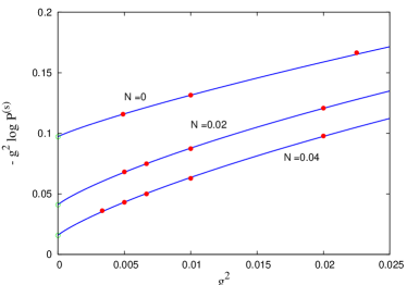
Figure 15: The quantity $-g^{2}\mathop{\rm ln}\nolimits{\cal P}^{(s)}$ viewed as a function of $g^{2}$ at fixed $N$ and $E=0.5$.

It is important to point out that we do not consider $\gamma$ as a free parameter of the fit. Rather, we use the following result of Ref. prefactor : for the sphaleron–mediated processes, such as ours, $\gamma=1$ at $N=0$ (vacuum initial state), and $\gamma=2$ at $N\neq 0$. Some of the numerical results (points) together with their fits by the formula (49) (lines) are shown in Fig. 15. The graphs are drawn for three different values of $N$ and $E=0.5$. Apparently, our data are well approximated by the asymptotic (49). To get the value of the suppression exponent $F$, one extrapolates the curves in Fig. 15 to the point $g^{2}=0$, where the quantum mechanical results should coincide with the semiclassical ones. The error of the extrapolation arises mainly from the disregarded terms proportional to the higher powers of $g^{2}$. One reduces such errors by computing the reflection probability at the smallest possible $g^{2}$. In practice we used two values of the semiclassical parameter in each fit, namely, $g=0.1,\;0.07$ at $N=0$, and $g=0.1,\;0.08$ at $N=0.02,\;0.04$. The extrapolation error is determined by pouring some additional points into the fit; it varies from $\delta F\sim 10^{-2}$ at small $E$ to $\delta F\sim 10^{-4}$ at $E\sim 1$. It matches with the estimate $O(g^{4})\sim 10^{-4}$ of higher–order terms of the semiclassical expansion which are neglected in Eq. (49).

Our final results for the suppression exponent $F(E,N)$ extracted from the numerical solution of the Schrödinger equation are presented in Fig. 13 (points with error bars standing for the accuracy of the extrapolation). The quantum mechanical results are in very good agreement with the semiclassical ones (lines). This justifies the semiclassical approach presented in this paper.

VI Summary and discussion

In this paper we tested the semiclassical method of complex trajectories in the regime of chaotic dynamical tunneling. We studied a particular example, over-barrier reflection in the two-dimensional waveguide model (2). The initial state of the process was fixed by the total energy ${\cal E}$ and occupation number ${\cal N}$ of the transverse oscillatory motion. We calculated the suppression exponent of the process both semiclassically and by solving exactly the full Schrödinger equation. The two approaches show very good agreement.

The tunneling trajectories in our semiclassical approach are obtained as solutions to the boundary value problem (21). We advocated a particular method for finding these solutions. It consists of two important ingredients:
(i) determination of the solution at some values of the initial–state parameters $E$, $N$;
(ii) gradual deformation of the solution to other $E$, $N$.

The deformation procedure (ii) was developed in Refs. Kuznetsov:1997az ; Bonini:1999kj . The advantages of this procedure are the simplicity of numerical implementation and generality. It can be applied efficiently to systems with many degrees of freedom, including non–trivial models of field theory, see Ref. Bezrukov:2003er .

On the other hand, a generic approach for performing the step (i) was missing so far. In this paper we proposed the systematic procedure which fills this gap. The procedure enables one to obtain the complex tunneling trajectories starting from the real classical solutions. It is based on the $\epsilon$–regularization method of Refs. Bezrukov:2003yf . Our procedure appears to be generic. It can be applied to any process which proceeds classically at some values of the initial–state parameters (at large $N$ in our case) and becomes exponentially suppressed at other values.

The process we studied is a particular example of chaotic tunneling. The chaoticity manifests itself in the infinite number of tunneling solutions. Our procedure, which connects the tunneling solutions to the classical ones, turns to be highly efficient in this situation. Namely, it enables one to classify the tunneling trajectories on the basis of the analysis of the classical dynamics. This was demonstrated explicitly in the present paper.

In addition, we proposed a heuristic criterion for sorting out the least suppressed tunneling trajectories basing on the classification of their classical progenitors. Hopefully, this criterion will be useful for the processes in other dynamical systems as well.

Another interesting feature of our setup is the phenomenon of optimal tunneling. Namely, the suppression exponent $F$ considered as a function of energy $E$ at fixed $N$ is non-monotonic. It attains the local minimum at $E\approx 0.5$ which is thus (locally) the optimal energy for tunneling. It is worth stressing that this behavior of the suppression exponent is unrelated to the quantum interference, which was neglected in the semiclassical analysis and eliminated from the exact quantum computations. Another example of tunneling process with non-monotonic dependence of the suppression exponent on energy is considered in Ref. wigles .

Let us mention some open issues.

The method of complex trajectories is known to suffer, in general, from the difficulties related to the Stokes phenomenon Berry:1972 ; Adachi:1986 . The essence of this phenomenon is that solutions of the tunneling problem may be unphysical in some regions of the parameter space; the contributions of such solutions to the tunneling probability should be dropped out. Presently, there are no generic criteria for distinguishing between the physical and unphysical solutions. One notes that the method we put forward in this paper trivially excludes some of the unphysical solutions. Indeed, we start from the classically allowed region of initial data (large $N$) where the physical solutions are precisely the real–valued classical trajectories. At the second step we relate these solutions to the complex tunneling trajectories; thus, we exclude the branches of unphysical solutions which are complex–valued deep inside the classically allowed region of initial data. Due to this “automatic” criterion, we did not see any manifestations of the Stokes phenomenon in the semiclassical calculations presented above. We remark, however, that the tunneling process we studied is the simplest one from the point of view of the Stokes phenomenon; the above “automatic”exclusion of unphysical solutions is insufficient in somewhat more involved situations. Two aspects of our model simplify the analysis. First, we observed that the tunneling solutions obtained from the real classical trajectories of a given topology $\alpha$ form a single smooth branch which covers the entire range of initial data. Second, we showed that the hierarchy of the suppression exponents $F_{\alpha}$ is the same at different values of $E$, $N$. These two observations allowed us to identify a single smooth branch of physical solutions which give the dominant contribution to the tunneling probability. In other models (see, e.g., Ref. wigles ) the solutions obtained by small deformations from different parts of the classically allowed region of initial data may correspond to different smooth branches of complex trajectories. Each of these branches may be physical and dominant in some region of the initial data plane, and unphysical or sub-dominant in other regions. If this is the case, some method of treating the Stokes phenomenon Shudo:1996 ; Ribeiro:2004 ; Parisio:2005 should be exploited.

The approach adopted in this paper was to perform the evaluation of the tunneling probability as the systematic semiclassical expansion in terms of $g^{2}$. We have calculated the leading term (suppression exponent). It is of interest to develop a method for calculating the sub-leading terms, in particular, the pre-exponential factor $A$, see Eq. (1). Presumably, this can be done along the lines of Ref. prefactor . An important problem which should be solved here is how to cope with the infinite number of tunneling paths, whose suppressions can be arbitrarily close to the limiting value. In particular, one has to understand whether the contributions of all the paths should be summed up or the correct value of the prefactor is determined by a sort of limiting procedure similar to the one we used to obtain the suppression exponent.

Another question is the following one. While solving the Schrödinger equation we observed that at finite $g^{2}$ the dependence of the exact tunneling probability on energy is modulated by oscillations. We conjectured that they result from the quantum interference of different tunneling trajectories. In the true semiclassical limit $g^{2}\to 0$ the above oscillations become infinitely frequent and should be averaged over. In real physical situations one deals, however, with small but finite values of the semiclassical parameter $g^{2}$. Thus it would be interesting to reproduce the interference pattern mentioned above in the semiclassical approach. As suggested by Refs. Shudo:1996 ; Shudo1995_1 ; Onishi2003 this could be done by summing up the contributions of various tunneling trajectories at finite $g^{2}$. We leave this investigation for the future work.

Acknowledgments

We are indebted to F.L. Bezrukov and V.A. Rubakov for useful discussions and helpful suggestions. This work was supported in part by the RFBR grant 05-02-17363, Grants of the President of Russian Federtion NS-7293.2006.2 (government contract 02.445.11.7370), MK-2563.2006.2 (D.L.), MK-2205.2005.2 (S.S.), the Grants of the Russian Science Support Foundation (D.L. and S.S.), the Fellowship of the “Dynasty” Foundation (awarded by the Scientific board of ICPFM) (A.P.) and the INTAS grant YS 03-55-2362 (D.L.). D.L. is grateful to the Universite Libre de Bruxelles and to EPFL, Lausanne, for the hospitality during his visits. The numerical calculations were performed on the Computational cluster of the Theoretical division of INR RAS.

Appendix A A method to obtain the unstable solutions

In this Appendix we describe the numerical method used to obtain the limiting tunneling trajectories considered in Sec. IV, namely, the ones ending up at the far sphaleron at late times. The main problem here is the instability of the trajectories in question.

Our main idea is to add the following term to the action functional,

$$S[{\boldsymbol{x}}]\mapsto S[{\boldsymbol{x}}]+iM(x(t_{f})-x_{f}^{0})^{2}\;,$$ (50)

where $x(t_{f})$ stands for the final value of the coordinate $x$, while $M>0$, $x_{f}^{0}$ are real parameters. For a given trajectory the term (50) leads to additional contribution to the suppression exponent,

$$\Delta F=2M(x(t_{f})-x_{f}^{0})^{2}\;.$$ (51)

The introduction of the above term induces the following modification of the boundary conditions (21c),

$$\mathop{\rm Im}\nolimits x(t_{f})=0\;,$$ (52a)

$$\mathop{\rm Im}\nolimits\dot{x}(t_{f})=-2M(x(t_{f})-x_{f}^{0})\;.$$ (52b)

This can be shown using the systematic approach of Refs. Bezrukov:2003yf ; prefactor ; wigles . At large positive $M$ the term (51) fixes the value of the final $x$-coordinate of the solutions to be close to $x_{f}^{0}$. For our purposes we choose $x_{f}^{0}$ to be in the vicinity of the far sphaleron, $x_{f}^{0}=-1$. Solutions which approach the far sphaleron at late times are obtained in the following way. One finds a solution to the original equations of motion which spends finite time on the far sphaleron, and cuts it at the moment $t=t_{f}$ when it is still at $x\approx-1$. Using this trajectory as the zeroth–order approximation, one applies the Newton–Raphson algorithm and obtains the solution satisfying the boundary conditions (52). The latter solution is defined inside the interval $t\in[t_{i},t_{f}]$. The next step is to continue the solution to a larger time interval by gradually increasing the value of $t_{f}$ and deforming the tunneling solution. As a result, one obtains the solution living at the far sphaleron for an arbitrarily long time.

The solution obtained in this way does not, strictly speaking, satisfy the boundary conditions (21c) of the tunneling problem. In order to restore the original boundary conditions (21c) one should, in principle, investigate the dependence $x_{f}(x_{f}^{0})$ and find the value of $x_{f}^{0}$ which solves the equations $x_{f}(x_{f}^{0})=x_{f}^{0}$. However, it is not necessary in our case: at late times the limiting solution is almost real, so one obtains $\mathop{\rm Im}\nolimits\dot{x}_{f}\approx 0$ automatically.

Appendix B Numerical solution of the Schrödinger equation

Here we present the numerical formulation of the problem (36), (39), (40). First of all, the range of the translatory coordinate should be bounded, $-L\leq X\leq L$, as well as the oscillator excitation number, $n<N_{y}$. Besides, we introduce the uniform lattice with spacing $\Delta$,

$$X_{k}=-L+(k+1)\Delta\;,\qquad k=-1,\dots,N_{x}+1\;,$$

where $N_{x}=-2+2L/\Delta$. The Taylor series expansion gives,

$$\frac{1}{\Delta^{2}}\left[\psi_{k+1}-2\psi_{k}+\psi_{k-1}\right]=\\ =\psi_{k}^{\prime\prime}+\frac{\Delta^{2}}{12}\psi_{k}^{(IV)}+O(\Delta^{4})\;.$$ (53)

By $\psi_{k}^{\prime\prime}$ and $\psi_{k}^{(IV)}$ we denote the second and fourth derivatives of $\psi$ at $X=X_{k}$. Note that the index $n$ is suppressed: hereafter we use the matrix notations. From Eq. (36) $\psi_{k}^{\prime\prime}=A_{k}\psi_{k}$; for the fourth derivative one writes,

$$\psi_{k}^{(IV)} =\frac{1}{\Delta^{2}}\left[\psi_{k+1}^{\prime\prime}-2\psi_{k}^{\prime\prime}+\psi_{k-1}^{\prime\prime}\right]+O(\Delta^{2})$$

$$=\frac{1}{\Delta^{2}}\left[A_{k+1}\psi_{k+1}-2A_{k}\psi_{k}+A_{k-1}\psi_{k-1}\right]+O(\Delta^{2})\;.$$

Substituting the above expressions into Eq. (53), one gets the forth–order Numerov–Cowling approximation for Eq. (36),

$$\left(1-\frac{\Delta^{2}}{12}A_{k+1}\right)\psi_{k+1}-\left(2+\frac{5\Delta^{2}}{6}A_{k}\right)\psi_{k}+\\ +\left(1-\frac{\Delta^{2}}{12}A_{k-1}\right)\psi_{k-1}=0\;,\;\;\;\;k=0,\dots,N_{x}\;.$$ (54)

It is worth noting that Eq. (54) supports the discrete probability current, which is conserved exactly,

$$J^{(\mathrm{d})}=\frac{1}{\Delta}\mathrm{Im}\,\psi_{k}^{+}\left(1-\frac{\Delta^{2}}{12}A_{k}\right)\left(1-\frac{\Delta^{2}}{12}A_{k+1}\right)\psi_{k+1}\;.$$ (55)

This conservation law was used to estimate the round–off errors.

The boundary conditions (39), (40) are imposed at the very last and first sites, $k=N_{x}+1$ and $-1$ respectively. One notes that the asymptotic formula (37) holds in the discrete case as well, provided the continuum dispersion relation (38) is replaced with the discrete one,

$$P_{n}\to P_{n}^{(\mathrm{d})}=\frac{2}{\Delta}\mathrm{arcsin}\frac{P_{n}\Delta}{2\sqrt{1+P_{n}^{2}\Delta^{2}/12}}\;.$$

Consequently, one rewrites Eqs. (39), (40) as

$$\psi_{n,N_{x}+1}-\mathrm{e}^{iP_{n}^{(\mathrm{d})}\Delta}\psi_{n,N_{x}}=\delta_{n,{\cal N}}\mathrm{e}^{-iP_{n}^{(\mathrm{d})}L}(1-\mathrm{e}^{2iP_{n}^{(\mathrm{d})}\Delta})\;,$$

$$\psi_{n,0}-\mathrm{e}^{-iP_{n}^{(\mathrm{d})}\Delta}\psi_{n,-1}=0\;.$$ (56)

These relations together with Eq. (54) form a system of $N_{y}(N_{x}+3)$ linear equations for the same number of unknowns $\psi_{n,k}$. After solving them, one calculates the reflection probability by making use of the discrete current,

$${\cal P}=\frac{|J^{(\mathrm{d,out})}|}{|J^{(\mathrm{d,in})}|}\;,$$

where $J^{(\mathrm{d,in})}$ and $J^{(\mathrm{d,out})}$ are the incoming and outgoing currents at $k=N_{x}+1$,

$$J^{(\mathrm{d,out})}=\frac{1}{\Delta}\sum_{n<{\cal E}-1/2}\frac{\sin(P_{n}^{(\mathrm{d})}\Delta)|r_{n}^{+}|^{2}}{\left(1-\frac{1}{3}\sin^{2}\frac{P_{n}^{(d)}\Delta}{2}\right)^{2}}\;,$$

$$J^{(\mathrm{d,in})}=-\frac{1}{\Delta}\frac{\sin(P_{\cal N}^{(\mathrm{d})}\Delta)}{\left(1-\frac{1}{3}\sin^{2}\frac{P_{\cal N}^{(d)}\Delta}{2}\right)^{2}}\;,$$

while the reflection amplitudes $r_{n}^{+}$ are extracted from the wave function,

$$r_{n}^{+}=\frac{\psi_{n,N_{x}+1}-\mathrm{e}^{-iP_{n}^{(\mathrm{d})}\Delta}\psi_{n,N_{x}}}{1-\mathrm{e}^{-2iP_{n}^{(\mathrm{d})}\Delta}}\cdot\mathrm{e}^{-iP_{n}^{(\mathrm{d})}L}\;.$$

We will see shortly that the finite difference approximation works well only if the numbers of the lattice points and oscillator levels are large. Typically, $N_{x}\sim 10000$, $N_{y}\sim 500$, and the system (56), (54) contains $N_{y}(N_{x}+3)\sim 5\cdot 10^{6}$ equations. Such an enormous system of equations cannot be solved with the general algorithms of linear algebra. So, we took advantage of the special form of Eqs. (54). Namely, the $k$-th matrix equation relates the vector $\psi_{k}$ to the unknowns at the adjacent sites $\psi_{k-1}$ and $\psi_{k+1}$ only; by performing numerically the matrix inversion it can be recast in the form

$$\psi_{k}=L_{k}\psi_{k-1}+R_{k}\psi_{k+1}\;,$$

where $L_{k}$ an $R_{k}$ are the $N_{y}\times N_{y}$ matrices. One substitutes the above formula into the other equations of the system (54), thus excluding $\psi_{k}$, as well as the $k$–th matrix equation. Performing this operation repeatedly, one ends up with a few matrix equations, which can be solved in a straightforward manner by the $LU$ decomposition method. It is worth pointing out that the variables $\psi_{k}$ and $\psi_{q}$ which are not neighbors to each other, can be excluded in parallel, so that the above algorithm is suitable for the multiprocessor machines or computational clusters. The reader interested in the details of the algorithm should address Refs. Bonini:1999kj , Levkov:2002qg , or our Fortran 90 code program , which hopefully can be executed on other machines.

Before proceeding to the actual calculations, one makes sure that the parameters of the lattice are chosen properly, so that the truncation and discretization errors are kept under control. Our purpose is to get the quantum mechanical results in the semiclassical region $g^{2}\to 0$. Therefore, it is convenient to account explicitly for the dependence of the lattice parameters on $g$. The truncation $L$ of the translatory coordinate is fixed by the condition that the interaction represented by the function $\tilde{a}(X)$ is small enough at $X=L$. Taking into account the scaling (35) of $\tilde{a}(X)$ with $g$, one obtains the formula

$$L=\tilde{L}/g\;,$$

where $\tilde{L}$ is fixed and large. In the practical calculations we used the value $\tilde{L}=12$, which is large enough as $a(\tilde{L})\sim 10^{-31}$: at $g>0.07$ this number is smaller than the absolute values of the reflection amplitudes, the latter exceeding $10^{-8}$. We have chosen the truncation of the oscillator levels in accordance with the condition that the occupation number of the last mode is negligible,

$$\sum_{k}|\psi_{N_{y}-1,k}|<10^{-30}\;;$$

this inequality was satisfied with $N_{y}$ typically ranging in between $200$ and $500$. The last parameter, the lattice spacing $\Delta$, should be several times smaller than the minimal De Broglie wavelength; we have found that the formula

$$\Delta=0.3\cdot\min_{n}\frac{1}{|P_{n}|}$$

works well enough producing relative errors of order $10^{-4}$.

The fact that the discretization corresponds to the relative rather than absolute errors can be understood as follows. The equations (54) and (56) may be regarded as the ones describing reflection of a quantum particle in a kind of crystal. Indeed, the substitution $\phi_{k}=\left(1-\frac{\Delta^{2}}{12}A_{k}\right)\psi_{k}$ brings Eq. (54) into the form ${\cal H}^{(d)}\phi=0$, where $\phi$ is the column composed of $\phi_{k}$, and ${\cal H}^{(d)}$ is a Hermitean linear operator. The probability of reflection in a crystal is exponentially small due to the same dynamical reasons as in the continuum case. One concludes that the finite value of $\Delta$ gives rise to corrections to the suppression exponent, rather than to the reflection probability itself, i.e. it produces relative discretization errors. We have checked the above physical considerations by performing calculations on the lattices with different cutoffs and lattice spacings. The overall conclusion is that, indeed, the discretization effects result in relative errors of order $10^{-4}$, while the truncation errors are always negligible. We kept the round–off errors under control by exploiting the current conservation law (55), which was checked to hold with precision better than $10^{-12}$.

References

-
(1)
A. M. Perelomov, V. S. Popov and M. V. Terent’ev, ZHETF 51, 309
(1966).
V. S. Popov, V. Kuznetsov and A. M. Perelomov, ZHETF 53, 331 (1967). - (2) W. H. Miller, Adv. Chem. Phys. 25, 69 (1974).
-
(3)
I. Y. Kobzarev, L. B. Okun and M. B. Voloshin,
Sov. J. Nucl. Phys. 20, 644 (1975)
[Yad. Fiz. 20, 1229 (1974)].
S. R. Coleman, Phys. Rev. D 15, 2929 (1977) [Erratum-ibid. D 16, 1248 (1977)]. - (4) M. Davis and E. Heller, J.Chem.Phys. 75, 246 (1981).
-
(5)
M. Wilkinson, Physica 21D, 341 (1986).
S. Takada and H. Nakamura, J. Chem. Phys. 100, 98 (1994).
S. Takada, P.N. Walker and M. Wilkinson, Phys. Rev. A 52, 3546 (1995).
S. Takada, J. Chem. Phys. 104, 3742 (1996). -
(6)
T. Banks, C. M. Bender and T. T. Wu,
Phys. Rev. D 8, 3346 (1973).
T. Banks and C. M. Bender, Phys. Rev. D 8, 3366 (1973). - (7) V. A. Rubakov, D. T. Son and P. G. Tinyakov, Phys. Lett. B 287, 342 (1992).
- (8) A. N. Kuznetsov and P. G. Tinyakov, Phys. Rev. D 56, 1156 (1997) [arXiv:hep-ph/9703256].
- (9) F. Bezrukov, D. Levkov, C. Rebbi, V. A. Rubakov and P. Tinyakov, Phys. Rev. D 68, 036005 (2003) [arXiv:hep-ph/0304180]; Phys. Lett. B 574, 75 (2003) [arXiv:hep-ph/0305300].
- (10) D. G. Levkov and S. M. Sibiryakov, Phys. Rev. D 71, 025001 (2005) [arXiv:hep-th/0410198]; JETP Lett. 81, 53 (2005) [Pisma Zh. Eksp. Teor. Fiz. 81, 60 (2005)] [arXiv:hep-th/0412253].
- (11) I. Affleck, Nucl. Phys. B 191, 429 (1981).
- (12) M. V. Berry and K. E. Mount, Rep. Prog. Phys. 35, 315 (1972).
- (13) S. Adachi, Ann.Phys. 195, 45 (1989).
- (14) A. Shudo, K. S. Ikeda, Phys.Rev.Lett. 76, 4151 (1996).
- (15) A.D. Ribeiro, M.A.M. de Aguiar, M. Baranger, Phys. Rev. E 69, 066204 (2004).
- (16) F. Parisio, M.A.M. de Aguiar, J. Phys. A: Math. Gen. 38, 9317 (2005).
- (17) O. Bohigas, S. Tomsovic and D. Ullmo, Phys. Rep. 223, 43 (1993).
-
(18)
E. Doron and S. D. Frischat,
Phys. Rev. Lett. 75, 3661 (1995);
S. D. Frischat and E. Doron, Phys. Rev. E 57, 1421 (1998). - (19) A. Mouchet, C. Miniatura, R. Kaiser, B. Grémaud, D. Delande, Phys. Rev. E 64, 016221 (2001).
- (20) A. Shudo, K.S. Ikeda, Phys. Rev. Lett. 74, 682 (1995); Physica D 115, 234 (1998).
- (21) A. Shudo, Y. Ishii and K. S. Ikeda, J. Phys. A 35, L225 (2002).
- (22) T. Onishi, A. Shudo, K.S. Ikeda and K. Takahashi, Phys. Rev. E 68, 056211 (2003).
- (23) T.Van Voorhis, E.J. Heller, Phys. Rev. A 66, 050501(R) (2002).
-
(24)
B. Eckhardt, C. Jung J. Phys. A 19, L829 (1986);
B. Eckhardt, Physica D 33, 89 (1988);
P. Gaspard, S.A. Rice, J. Chem. Phys. 90, 2225 (1988). -
(25)
V. I. Zakharov, Nucl. Phys. B 353, 683 (1991);
Phys. Rev. Lett. 67, 3650 (1991).
G. Veneziano, Mod. Phys. Lett. A 7, 1661 (1992). - (26) M. Maggiore and M. A. Shifman, Phys. Rev. D 46, 3550 (1992).
- (27) M. B. Voloshin, Phys. Rev. D 49, 2014 (1994).
- (28) V. A. Rubakov and D. T. Son, Nucl. Phys. B 424, 55 (1994) [arXiv:hep-ph/9401257].
- (29) C. S. Drew, S. C. Creagh and R. H. Tew, Phys. Rev. A 72, 062501 (2005).
- (30) F. Bezrukov and D. Levkov, arXiv:quant-ph/0301022; J. Exp. Theor. Phys. 98, 820 (2004) [Zh. Eksp. Teor. Fiz. 125, 938 (2004)] [arXiv:quant-ph/0312144].
- (31) K. Takahashi and K.S. Ikeda, J. Phys. A 36, 7953 (2003); Europhys. Lett. 71, 193 (2005).
- (32) F. R. Klinkhamer and N. S. Manton, Phys. Rev. D 30, 2212 (1984).
- (33) G. F. Bonini, A. G. Cohen, C. Rebbi and V. A. Rubakov, Phys. Rev. D 60, 076004 (1999) [arXiv:hep-ph/9901226]; arXiv:quant-ph/9901062.
- (34) D. G. Levkov, A. G. Panin and S. M. Sibiryakov, “Tunneling via unstable semiclassical solutions,” arXiv:0707.0433 [quant-ph].
- (35) D. G. Levkov, A. G. Panin and S. M. Sibiryakov, Phys. Rev. A 76, 032114 (2007) [arXiv:0704.0409].
- (36) W.H. Press, S.A. Teukolsky, W.T. Vetterling, B.P. Flannery, “Numerical recipes in C: the art of scientific computing”, Cambridge University Press, 1992.
- (37) A.L. Xavier Jr., M.A.M. de Aguiar, Ann. Phys 252, 458 (1996).
- (38) D. Levkov, C. Rebbi and V. A. Rubakov, Phys. Rev. D 66, 083516 (2002) [arXiv:gr-qc/0206028].
- (39) http://solver.inr.ac.ru