Saturable discrete vector solitons in one-dimensional photonic lattices

Abstract

Localized vectorial modes, with equal frequencies and mutually orthogonal polarizations, are investigated both analytically and experimentally in a one-dimensional photonic lattice with saturable nonlinearity. It is shown that these modes may span over many lattice elements and that energy transfer among the two components is both phase and intensity dependent. The transverse electrically polarized mode exhibits a single-hump structure and spreads in cascades in saturation, while the transverse magnetically polarized mode exhibits splitting into a two-hump structure. Experimentally such discrete vector solitons are observed in lithium niobate lattices for both coherent and mutually incoherent excitations.

Solitons or stable strongly localized nonlinear structures, which can elastically interact with linear waves and other solitons, have been studied in various systems in nature, ranging from astrophysics 1 and ocean waves 2 , down to Josephson junctions 3 and nanowires 4 . These localized structures exist due to an exact balance between two or more counteracting effects such as, for example, dispersion and nonlinearity in the temporal domain book . In the optical domain, solitons may exist in specific materials, such as Kerr and photorefractive ones 6 ; 7 . On the other hand, solitons occur in different forms like incoherent, discrete, and vector solitons, which are not directly related to a particular material book . Vector solitons are composite structures that consist of two or more components which mutually self-trap in a nonlinear medium. Importantly, the individual components decay in isolation. The existence of vector solitons was first suggested by Manakov in 1974 9 . Later on, vector solitons have been, for example, studied in carbon disulfide 10 and photorefractive crystals 11 . In periodic nonlinear systems, the so-called discrete solitons exist due to the balance between nonlinearity and discreteness DS . They have been observed in diverse physical configurations such as biological systems, charge-transfer solids, Josephson junctions, micromechanical oscillator arrays, and photonic lattices. However, nonlinear optics has overtaken a primacy in the nowadays soliton related research 15 ; 16 due to a rather mature technology of photonic lattice fabrication. Such photonic crystals have periodic distributions of the refractive index and light propagation is associated with allowed bands and forbidden gaps, analog to propagation of electrons in crystalline lattices OE05 .

One-dimensional (1D) discrete vector solitons (DVS) originating from the first band have been already investigated both analytically 17 ; 18 and experimentally 19 in nonlinear cubic waveguide arrays (WA). The two-dimensional case was studied, too 20 . Finally, multi-band vector solitons, in which individual components stem from different bands, were also recently suggested and demonstrated 21 . The aim of the present study is to investigate DVS in media with saturable nonlinearity. Prime examples of such media are photonic lattices in photorefractive crystals. Additionally, semiconductors at higher light intensities also exhibit saturation 22 . It has been shown that saturation, which may occur in a cascade manner in discrete systems 23 , is responsible for the existence of multiple zeros of the Peierls-Nabarro potential, leading to free steering of large amplitude solitons, and stable propagation of inter-site modes in 1D and 2D systems 24 . Various species of two-component saturable DVS have been investigated recently, where it was assumed that both components have the same polarization and different frequencies 25 . In what follows we are interested in the situation where the components have the same frequency but differ in polarization.

By following the procedures outlined in Refs. 11 ; 26 , assuming only nearest neighbor interactions, and by using the slowly varying envelope approximation, one may obtain the following model equations:

$$i\frac{\partial u_{n}}{\partial\xi}+L_{u}u_{n}-\beta\ \frac{\left(u_{n}+s_{2}Bv_{n}\right)}{\left(1+|u_{n}|^{2}+s_{1}|v_{n}|^{2}\right)}=0,$$

$$i\frac{\partial v_{n}}{\partial\xi}+L_{v}v_{n}-\,\beta\ \frac{\left(s_{1}Bu_{n}+s_{3}Av_{n}\right)}{\left(1+|u_{n}|^{2}+s_{1}|v_{n}|^{2}\right)}=0,$$ (1)

where $L_{u}u_{n}=(C_{0}-\Delta k)u_{n}+V_{0}(u_{n+1}+u_{n-1})$ and $L_{v}v_{n}=[C_{0}v_{n}+V_{0}(v_{n+1}+v_{n-1})]/s_{1}$. Here $\xi$ is the normalized propagation coordinate ($y$ in the experiment). The normalized envelopes $u_{n}$ and $v_{n}$ correspond to transverse electrically (TE) and magnetically (TM) polarized fields, respectively. The parameter $\beta$ represents the nonlinear coefficient, the normalized coupling constant is denoted by $V_{0}$, $\Delta k$ is the normalized difference of TE and TM wave numbers, whereas $C_{0}$ can be regarded as a normalized propagation constant. By defining birefringence $\Delta n=n_{x}-n_{z}$ and average refractive index $n_{0}=(n_{x}+n_{z})/2$, we write the function $s_{j}\approx 1+j\Delta n/{n_{0}}$. Finally, $A=r_{xxz}/r_{zzz}$ and $B=r_{xzx}/r_{zzz}$, where $r_{ijk}$ denote the components of the Pockels tensor 11 . One may notice that in general, alike DVS in Kerr media 18 ; 19 ; 20 , in our situation there exists no possibility to separate cross-phase and four-wave mixing effects. A conserved quantity of this model is the total power, $P=\sum_{n}\left(|u_{n}|^{2}+s_{1}|v_{n}|^{2}\right)=P_{u}+s_{1}P_{v}$. By using (1), it can be shown that ${\partial P}/{\partial\xi}=0$ implies:

$$\frac{\partial P_{u}}{\partial\xi}=-s_{1}\frac{\partial P_{v}}{\partial\xi}=2\beta s_{2}B\sum_{n}\frac{\mathrm{Im}(v_{n}u_{n}^{*})}{\left(1+|u_{n}|^{2}+s_{1}|v_{n}|^{2}\right)}\,.$$ (2)

This expression gives us information on the energy (power) exchange among the TE and TM components which clearly will depend on the total level of power in each waveguide. By considering a one-channel constant-amplitude propagation of the form $u_{0}(\xi)=u_{0}\exp[i(\lambda_{u}\xi+\phi_{u})]$ and $v_{0}(\xi)=v_{0}\exp[i(\lambda_{v}\xi+\phi_{v})]$, where $\lambda_{i}$ and $\phi_{i}$ correspond to the respective propagation constants and initial phases, respectively, we obtain the following expression for the power transfer: $\partial P_{u}/\partial\xi\sim\sin(\Delta\lambda\xi+\Delta\phi)$, where $\Delta\lambda=\lambda_{v}-\lambda_{u}$ and $\Delta\phi=\phi_{v}-\phi_{u}$. By assuming only a linear and local dependence of the propagation constants, from (1) we get: $\lambda_{u}\approx C_{0}-\Delta k,\lambda_{v}\approx C_{0}/s_{1}$, which results in $\Delta\lambda\approx\Delta k$. If the components are initially in phase ($\Delta\phi=0$), the power transfer will be initially towards the TE mode provided that $\Delta k>0$, and towards the TM mode otherwise 18 .

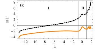
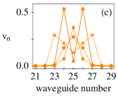
Figure 1: (Color online). (a) TE (dashed line) and TM (continuous line) powers as a function of the propagation constant. Vertical lines separate regions. (b) and (c) TE and TM profiles, respectively: Diamonds, squares, triangles and stars correspond to $\lambda=-5,-1,0$, and $1.1$, respectively. $C_{0}=\Delta k=\beta=10,\ V_{0}=1$.

To gain a theoretical background of the model (1), we use a Newton-Raphson method to find coupled localized stationary solutions of the form: $u_{n}(\xi)=u_{n}\exp(i\lambda_{u}\xi)$ and $v_{n}(\xi)=v_{n}\exp(i\lambda_{v}\xi)$, with $u_{n},v_{n}\in\Re$. For the sake of simplicity we assume $\lambda_{u}=\lambda_{v}\equiv\lambda$, which in turn disables the power exchange between DVS components [$\mathrm{Im}(v_{n}u_{n}^{*})=0$ in (2)]. These solutions may be regarded as the final stage of mode profiles after the DVS is formed. The power dependence of the two components on propagation constant, for the chosen set of experimentally achievable parameters 27 , is shown in Fig. 1(a) in a logarithmic scale. The region of existence of localized modes is between the low-amplitude and high-amplitude limits for the upper band edge plane wave 24 of the composed system of equations (1). In the present case, this region corresponds to $\sim\lambda\in\{-13,2\}$. Power of the TE mode always exceeds that of TM polarization and, interestingly, grows in a similar fashion as the power of the on-site mode A in Ref. 23 . For any $\lambda$, the TE mode is always a one-hump structure [see Fig. 1(b)] which spreads transversally in the region of saturation 23 . We may separate the $P\lambda$ diagram in smaller regions depending on the shape of the TM mode. In region I [$\sim\lambda\in\{-13,-0.6\}$], the TM mode corresponds to a one-hump structure [diamonds and squares in Fig. 1(c)]. In region II [$\sim\lambda\in\{-0.6,1\}$], the TM mode corresponds to a two-hump structure separated by only one site [triangles in Fig. 1(c)]. In the next regions, the TM mode increases its distance between the two humps in an odd number of waveguides [as an example, see stars in Fig. 1(c)].

While the total power increases, local saturation takes place 24 . As $\Delta k>0$, the TE mode is the one which gains power. Therefore the TE mode starts to increase its power locally together with the TM mode [region I in Fig. 1(a), diamonds and squares in Fig. 1(b,c)]. However, above some critical level of power [region II in Fig. 1(a), triangles in Fig. 1(b,c)] the local power in the center site is too high and the only possibility for the TM mode to exist is by exploring the neighborhood looking for a more stable configuration. Then, the TE mode further increases its power but now, due to saturation, by increasing the amplitudes in the next sites [see stars in Fig. 1(b)]. Again, the TM mode finds a new configuration which is initially stable, but now the separation between peaks consists of three sites [stars in Fig. 1(c)]. If we continue increasing the power we observe that the TE mode preserves its one-hump structure, by increasing its width, while the TM mode has a two-hump structure where the separation between peaks continuously increases. Therefore, the DVS is mostly TE polarized, except at tails which have a dominating TM polarization. The linear stability analysis of solutions coincides with the Vakhitov-Kolokolov criterion book : modes are stable for $\partial P/\partial\lambda>0$, and unstable otherwise. This implies that in region I solutions are always stable and, in the next regions, there exist both stable and unstable sub-regions [see Fig. 1(a)].

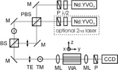
Figure 2: Scheme of the experimental setup.

To verify our theoretical predictions we use the experimental setup sketched in Fig. 2. A cw laser with wavelength 532 nm is split into two orthogonally polarized (TE and TM) mutually coherent waves with the help of a polarizing beam splitter PBS. Optionally, to allow for mutually incoherent interaction of the two components, a TM polarized wave can be provided by a second laser of the same wavelength. Input power is adjusted with a combination of half wave plate $\lambda$/2 and polarizer P. The two input beams are used to excite narrow single-channel TE and TM polarized modes of the WA by using a $40\times$ microscope lens ML. This nonlinear WA is fabricated in x-cut lithium niobate doped with copper. The length of our sample along the propagation y-direction is 11 mm and the array consists of 250 parallel titanium in-diffused waveguide channels that are 4 $\mu$m wide with a separation of 4.4 $\mu$m (grating period $\Lambda=8.4\,\mu$m) 28 . A second microscope lens ML images the intensity on the output face onto a CCD camera, where an additional polarizer P allows for independent observation of both TE and TM components of the DVS.

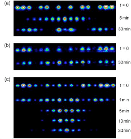
Figure 3: (Color online). Experimentally observed DVS for mutually coherent input beams. Temporal nonlinear evolution of (a) TE component alone ($P_{u}=150\,\mu$W); (b) TM component alone ($P_{v}=300\,\mu$W); and (c) both components together ($P_{u}=150\,\mu$W, P${}_{v}=300\,\mu$W).

The nonlinear dynamics of TE only, TM only, and both TE and TM modes (mutually coherent from the same light source) is presented in Fig. 3. Here we make use of the fact that in photorefractives the nonlinearity grows exponentially in time, $\beta(t)=\beta\,(1-\exp[-t/\tau])$, where $\tau$ is the dielectric response time 30 . Initially, after switching on the light ($t=0$), discrete diffraction is monitored for each situation. Although one may observe initial focusing of the TE mode within the first minutes in Fig. 3(a) (an even weaker effect is observed for TM), both modes alone are incapable to form a localized structure [Fig. 3(a,b)]. However, when both input polarizations are present [Fig. 3(c)] a five-channel wide DVS is formed after $t=30$ min and remains stable for longer times $t$.

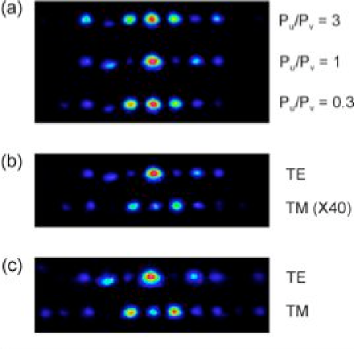
Figure 4: (Color online). Mode analysis of stationary DVS solitons. (a) Stationary output (total intensity TE + TM) of DVS for different power ratios $P_{u}/P_{v}$; (b) stationary TE and TM (amplified 40$\times$) polarized components for $P_{u}/P_{v}=1$; and (c) stationary TE and TM polarized components for $P_{u}/P_{v}=1$ when input TE beam is blocked after formation of the DVS.

Stationary images of DVS collected from the output facet of the sample for a fixed value of TE power and different values of TM power are presented in Fig. 4(a). As can be seen, the shape of the DVS slightly changes for different power ratios $P_{u}/P_{v}$. TE and TM polarized components for a power ratio $P_{u}/P_{v}=1$ (steady state) are shown in Fig. 4(b). As predicted, a dominating single-hump TE polarized component and a weaker double-humped TM component are observed. The role of the TM input polarization can be further analyzed by blocking the TE input after stable formation of the DVS in Fig. 4(c). Obviously the TM polarized input light transfers most of its energy to the TE component, forming a single-hump solution, while the remaining power is trapped in form of a two-hump solution. This energy transfer, from ordinary to extraordinary polarization (TM $\rightarrow$ TE), is due to a specific anisotropic nonlinearity in LiNbO₃ [in model (1), this corresponds to consider $\Delta k>0$]. The mechanism of coupling of orthogonally polarized modes is explained by writing holographic gratings due to photovoltaic currents. Light is anisotropically diffracted from these shifted gratings with polarization conversion, which leads to an energy exchange among the modes 29 .

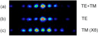
Figure 5: (Color online). Experimentally observed DVS for mutually incoherent input beams. (a) Stationary output of DVS [total intensity TE + TM] for $P_{u}/P_{v}=1.5$; (b) TE polarized component; and (c) TM polarized components (amplified 8$\times$).

Energy coupling of orthogonally polarized waves can be prevented by using mutually incoherent input beams ($B=0$). Experimentally this is realized by a second laser of the same wavelength (see Fig. 2), which now provides the TM polarized input beam, and corresponding results for the steady-state DVS formation are shown in Fig. 5. Again a two-hump structure is observed for the TM component, which now guides a significant part of the total power of the soliton.

In conclusion, we suggested a rather general theoretical model to describe saturable discrete vector solitons having orthogonally polarized components. Power transfer and coupling between TE and TM components is investigated as well as the corresponding localized stationary solutions. We discovered that these composite solitons might have different width and shape depending on the region of parameters. The dominating TE mode is single-humped while the weaker TM mode may exhibit both one- and two-hump structures. We confirm our findings experimentally by using either coherent or mutually incoherent excitations, where the latter is used to suppress energy coupling in formation of discrete vector solitons. Our experimental conditions match the region II of stationary solutions, a region with an intermediate level of power and highly localized solutions. This is because a one-channel input excites a strongly localized region of the array with high local intensity. The results obtained here could be useful in the codification of signals, filtered by polarization, in future all-optical communication networks.

We gratefully acknowledge financial support from BMBF (grant DIP-E6.1), DFG (grant KI482/8-1), and MNZŽSRS (grant 14-1034).

References

- (1) M. G. Abramyan, Astrophysics 22, 288 (1985).
- (2) T. P. Stanton and L. A. Ostrovsky, Geophys. Research Lett. 25, 2695 (1998).
- (3) J. Pfeiffer et al., Phys. Rev. Lett. 96, 034103 (2006).
- (4) R. El-Ganainy et al., Opt. Express 14, 2277 (2006).
- (5) Yu. S. Kivshar and G. P. Agrawal, Optical Solitons: From Fibers to Photonic Crystals (Academic, San Diego, 2003).
- (6) Y. N. Karamzin and A. P. Sukhorukov, Sov. Phys. JETP 41, 414 (1976).
- (7) M. Segev et al., Phys. Rev. Lett. 68, 923 (1992).
- (8) S. V. Manakov, Sov. Phys. JETP 38, 248 (1974).
- (9) N. Shalaby and A. J. Barthelemy, IEEE J. Quantum Electron. 28, 2376 (1992).
- (10) M. Segev et al. Opt. Lett. 20, 1764 (1995).
- (11) D. N. Christodoulides, F. Lederer, and Y. Silberberg, Nature 424, 817 (2003); D. K. Campbell, S. Flach, and Yu. S. Kivshar, Phys. Today 57 (1), 43 (2004).
- (12) D. N. Christodoulides and R. I. Joseph, Opt. Lett. 13, 794 (1988).
- (13) H. S. Eisenberg et al., Phys. Rev. Lett. 81, 3383 (1998).
- (14) J. W. Fleischer et al., Opt. Express 13, 1780 (2005).
- (15) S. Darmanyan et al., Phys. Rev. E57, 3520 (1998).
- (16) R. A. Vicencio, M. I. Molina, and Yu. S. Kivshar, Phys. Rev. E71, 056613 (2005); Opt. Lett. 29, 2905 (2004).
- (17) J. Meier et al., Phys. Rev. Lett. 91, 143907 (2003).
- (18) J. Hudock et al., Phys. Rev. E67, 056618 (2003); Z. Chen et al., Opt. Lett. 29, 1656 (2004).
- (19) O. Cohen et al., Phys. Rev. Lett. 91, 113901 (2003); D. Mandelik et al., Phys. Rev. Lett. 90, 053902 (2003).
- (20) J.-L. Coutaz and M. Kull, J. Opt. Soc. Am. B8, 95 (1991).
- (21) M. Stepić et al., Phys. Rev. E69, 066618 (2004).
- (22) Lj. Hadžievski et al., Phys. Rev. Lett. 93, 033901 (2004); R. A. Vicencio and M. Johansson, Phys. Rev. E73, 046602 (2006); E. Smirnov et al., Phys. Rev. E74, 065601 (2006).
- (23) E. P. Fitrakis et al., Phys. Rev. E74, 026605 (2006).
- (24) M. I. Carvalho et al., Phys. Rev. E53, R53 (1996).
- (25) In LiNbO3 , , , and .
- (26) F. Chen et al., Opt. Express 13, 4314 (2005).
- (27) M. Wesner et al., Phys. Rev. E64, 036613 (2001).
- (28) D. Kip and E. Krätzig, Opt. Lett. 17, 1563 (1992).