$N$-soliton solutions and perturbation theory for the derivative nonlinear Scrödinger equation with nonvanishing boundary conditions

Abstract

We present a simple approach for finding $N$-soliton solution and the corresponding Jost solutions of the derivative nonlinear Scrödinger equation with nonvanishing boundary conditions. Soliton perturbation theory based on the inverse scattering transform method is developed. As an application of the present theory we consider the action of the diffusive-type perturbation on a single bright/dark soliton.

1 Introduction

The derivative nonlinear Schrödinger equation (DNLSE) ($\alpha=\pm 1$)

$$i\partial_{t}u+\partial_{x}^{2}u+i\alpha\partial_{x}(|u|^{2}u)=0$$ (1)

has many physical applications, and, probably, the most important are in plasma physics and in nonlinear optic. First, equation (1) describes modulated small-amplitude nonlinear Alfvén waves in a low-$\beta$ (the ratio of kinetic to magnetic pressure) plasma, propagating parallel [1, 2, 3] or at a small angle [4, 5, 7] to the ambient magnetic field. The DNLS equation also describes large-amplitude magnetohydrodynamic waves in a high-$\beta$ plasma, propagating at an arbitrary angle to the ambient magnetic field [8]. In these cases $u$ denotes the transverse magnetic field perturbation normalized by the ambient magnetic field, where $t$ and $x$ are normalized time and space coordinates, respectively. Second, the DNLSE is related to the modified nonlinear Schrödinger equation (MNLSE)

$$i\partial_{\tau}\psi+\frac{\sigma}{2}\partial_{\xi}^{2}\psi+is\partial_{\xi}(|\psi|^{2}\psi)+|\psi|^{2}\psi=0$$ (2)

by a simple gaugelike transformation [9]

$$\psi(\xi,\tau)=u(x,t)\exp\left\{\frac{i}{4s^{4}}t+\frac{i\sigma}{2s^{2}}x\right\},$$ (3)

where $\sigma=\pm 1$ corresponds to the abnormal (normal) group velocity dispersion (GVD) region, $\xi=(\sigma x)/(2s)+t/(2s^{3})$, $\tau=(\sigma t)/(2s^{2})$. In turn, the MNLSE describes the propagation of ultrashort femtosecond nonlinear pulses in optical fibers, when the spectral width of the pulses becomes comparable with the carrier frequency, and, in addition to the usual Kerr nonlinearity, the effect of self-steepening of the pulse should be taken into account. In this case, $u$ is the normalized slowly varying amplitude of the complex field envelope, $t$ is the normalized propagation distance along the fiber, and $x$ is the normalized time measured in a frame of reference moving with the pulse at the group velocity.

Equation (1) is completed by the boundary conditions: vanishing ($u\rightarrow 0$ as $|x|\rightarrow\infty$) or nonvanishing ($|u|\rightarrow\rho=\mathrm{const}$ as $|x|\rightarrow\infty$) at infinity. In both cases the DNLSE is integrable by the inverse scattering transform (IST) [10, 11, 12, 13], and admits $N$-soliton solutions [14].

The nonvanishing boundary conditions (NVBC) are important in physical applications. For example, in space plasma physics the vanishing boundary conditions (VBC) are relevant only for the case of propagation of Alfvén waves strictly parallel to the ambient magnetic field. In nonlinear optics the NVBC can support propagation of dark solitons in both normal and abnormal GVD regions [15]. Unlike the nonlinear Schrödinger equation or the DNLSE with VBC, the DNLSE with NVBC admits simultaneous generation of breathers (solitons with internal oscillations) and one-parametric (nonoscillating) bright and/or dark solitons [16].

The IST formalism for the DNLSE with NVBC is much more complicated from the one for VBC. Analytical properties of the Jost solutions in this case are formulated on the Riemann sheets of the spectral parameter [11] and the corresponding direct and inverse scattering problems are rather involved. Recently, Chen and Lam [15] developed the IST for the DNLSE with NVBC by introducing an affine parameter to avoid constructing the Riemann sheets. Both approaches, however, encounter a difficulty when finding exact explicit $N$-soliton solutions. The reason is that the resulting solution $u$ containes the phase factor $\exp(i\eta^{+})$, where $\eta^{+}$ is some definite integral from $|u|^{2}$. Thus, the solution is written in an implicit form and only modulus of the solution can be obtained in that way. Though for simple one-parametric soliton solutions the phase $\eta^{+}$ can be calculated by direct integration, this procedure is obviously impracticable for $N$-soliton solutions. Instead, tricks leading to the explicit expression for $\eta^{+}$ were used in some particular cases: for the two-parametric one-soliton breather solution [15], and for the $N$-soliton with purely imaginary discrete spectral parameters (i. e. for pure bright and/or dark solitons) [17, 18]. Another approach based on Darboux/Bäclund transformations was developed by Steudel [14]. Apparently, Steudel was the first to obtain exact $N$-soliton solutions with explicitly calculated phases for the DNLSE with NVBC.

From the practical point of view, the completely integrable DNLSE (1) is an idealized model. In many physical applications, additional terms are often present in the DNLSE. They can include effects of the third-order linear dispersion, dissipation, influence of external forces, etc. . These terms violate the integrability, but being small in many important practical cases, they can be taken into account by perturbation theory. The most powerful perturbative technique, which fully uses the natural separation of the discrete and continuous (i.e., solitonic and radiative) degrees of freedom of the unperturbed DNLSE, is based on the IST. While the IST-based perturbation theory for the DNLSE with VBC was developed long ago [19], the analogous theory for nonvanishing boundary conditions was absent.

The aim of this paper is twofold. First, we present a relatively simple approach for finding exact explicit (i. e. with the phase) $N+M$-soliton ($N$ breathers and $M$ ”usual” bright and/or dark solitons in asymptotics) solutions of the DNLSE with NVBC and show that these solutions can be obtained without determining the phase factor $\exp(i\eta^{+})$. Thus, exact exotic solutions, describing, for instance, collisions between breathers, as well as collisions between pure bright/dark solitons and breathers can be written. Simultaneously, unlike the purely algebraic approach [14] based on Darboux transformation, the corresponding Jost solutions can also be obtained. A second aim is to present perturbation theory for solitons of the DNLSE with NVBC. We derive evolution equations for the scattering data (both solitonic and continuous) in the presence of perturbations. As an application of the present theory we consider the action of the diffusive-type perturbation on a single bright/dark soliton.

Without loss of generality, we will consider the NVBC in the form

$$u\rightarrow\rho\exp(\pm 2i\theta),\qquad\mbox{as}\qquad x\rightarrow\pm\infty.$$ (4)

We also put $\alpha=1$, since the case $\alpha=-1$ can be obtained from the former by a transformation $x\rightarrow-x$.

The paper is organized as follows. In section 2, we review a theory of the scattering transform for the DNLSE with NVBC. In section 3, we present the procedure to construct the general explicit $N+M$-soliton solution. Integrals of motion are obtained in section 4. The perturbation theory and its application are considered in sections 5 and 6, respectively. The conclusion is made in section 7.

2 Inverse scattering transform for the DNLSE with NVBC

In this section we present the theory of the scattering transform for the DNLSE with NVBC, following [15] with some modifications and specifications. Equation (1) can be written as the compatibility condition

$$\partial_{t}U-\partial_{x}V+[U,V]=0,$$ (5)

of two linear matrix equations (Kaup-Newell pair) [10]:

$$\partial_{x}M(x,t,\lambda)=UM(x,t,\lambda),$$ (6)

$$\partial_{t}M(x,t,\lambda)=VM(x,t,\lambda),$$ (7)

where $\lambda$ is a spectral parameter, and

$$U=-i\lambda^{2}\sigma_{3}+\lambda Q,\qquad\mbox{with }Q=\left(\begin{array}[]{cc}0&u\\ -u^{\ast}&0\end{array}\right),$$ (10)

$$V=-2i\lambda^{4}\sigma_{3}+2\lambda^{3}Q-i\lambda^{2}Q^{2}\sigma_{3}+\lambda Q^{3}-i\lambda Q_{z}\sigma_{3}$$ (11)

Consider the linear problem (6) for some fixed $t$. In terms of the matrix $U$ boundary conditions (4) can be rewritten as $\lim\limits_{x\rightarrow\pm\infty}U(x,\lambda)=U^{\pm}(\lambda)$, where

$$U^{\pm}=\left(\begin{array}[]{cc}-i\lambda^{2}&\rho\lambda e^{\pm 2i\theta}\\ -\rho\lambda e^{\mp 2i\theta}&i\lambda^{2}\end{array}\right).$$ (12)

Asymptotic solutions of (6) $E^{\pm}$ satisfy

$$\partial_{x}E^{\pm}=U^{\pm}E^{\pm}.$$ (13)

The double-valued function $K(\lambda)=\lambda\sqrt{\lambda^{2}+\rho^{2}}$ appears in the matrices $E^{\pm}$, and the analytical properties of solutions of Eq. (6) are formulated on the Riemann surface determined by the function $K(\lambda)$. The Riemann surface $\mathcal{S}$ consists of two sheets $\mathcal{S}^{+}$ and $\mathcal{S}^{-}$ of the complex $\lambda$–plane with branch cuts on the image axis from $-\infty$ to $-i\rho$ and from $i\rho$ to $\infty$. It is convenient to introduce an affine parameter $\zeta$ by a change of variable [15]

$$\lambda(\zeta)=\frac{1}{2}\left(\zeta-\frac{\rho^{2}}{\zeta}\right).$$ (14)

This transformation maps the sheets $\mathcal{S}^{\pm}$ onto $\mathrm{Im}\,\zeta>0$ and $\mathrm{Im}\,\zeta<0$ respectively and the real axis on the complex $\lambda$-plane into the real axis on the $\zeta$-plane. Under this,

$$E^{\pm}(x,\zeta)=e^{\pm i\theta\sigma_{3}}\left(\begin{array}[]{cc}1&-i\rho/\zeta\\ -i\rho/\zeta&1\end{array}\right)e^{-ik(\zeta)\sigma_{3}x}$$ (15)

where the single-valued function $k(\zeta)$ is determined by

$$k(\zeta)=\frac{1}{2}\left(\zeta+\frac{\rho^{2}}{\zeta}\right)\lambda(\zeta)$$ (16)

For $\mathrm{Im}\,\zeta=0$ denote by $M^{\,\pm}(x,\zeta)$ the $2\times 2$ matrix Jost solutions of (6), satisfying the boundary conditions

$$M^{\pm}\rightarrow E^{\pm}(x,\zeta),\qquad\mbox{as }x\rightarrow\pm\infty.$$ (17)

The corresponding integral equation can be obtained from (6) and (17)

$$M^{\pm}(x,\lambda)=E^{\pm}(x,\lambda)\mp i\lambda\int_{x}^{\pm\infty}E^{\pm}(x-y,\lambda)Q(y)M^{\pm}(y,\lambda)\,dy.$$ (18)

The matrix Jost solutions $M^{\,\pm}(x,\zeta)$ can be represented in the form $M^{-}=(\varphi,\bar{\varphi})$ and $M^{+}=(\bar{\psi},\psi)$, where $\varphi$ and $\psi$ are independent vector columns. The monodromy matrix $S(\zeta)$ relates the two fundamental solutions $M^{-}$ and $M^{+}$:

$$M^{-}(x,\zeta)=M^{+}(x,\zeta)S(\zeta).$$ (19)

The Jost coefficients are defined by

$$\varphi=a\bar{\psi}+b\psi,$$ (20)

$$\bar{\varphi}=-\bar{a}\psi+\bar{b}\bar{\psi},$$ (21)

so that the monodromy matrix is

$$S(\zeta)=\left(\begin{array}[]{cc}a(\zeta)&-\bar{b}(\zeta)\\ b(\zeta)&\bar{a}(\zeta)\end{array}\right),$$ (22)

where $a\bar{a}+b\bar{b}=1$. Matrices $M^{\pm}$ and $S$ have the parity symmetry properties

$$S(\zeta)=\sigma_{3}S(-\zeta)\sigma_{3},\qquad M^{\pm}(\zeta)=\sigma_{3}M^{\pm}(-\zeta)\sigma_{3},$$ (23)

and the conjugation symmetry properties

$$S(\zeta)=\sigma_{2}S^{\ast}(\zeta^{\ast})\sigma_{2},\qquad M^{\pm}(\zeta)=\sigma_{2}M^{\pm\,\ast}(\zeta^{\ast})\sigma_{2},$$ (24)

where $\sigma_{2}$ and $\sigma_{3}$ are Pauli matrices, so that $|a|^{2}+|b|^{2}=1$. In addition, since the scattering problem (6) possesses symmetry with respect to the inversion $\zeta\rightarrow\rho^{2}/\zeta$, the important involution properties are valid:

$$M^{\pm}(x,\rho^{2}/\zeta)=(\zeta/\rho)\sigma_{3}M^{\pm}(x,\zeta)\sigma_{2},$$ (25)

$$S(\rho^{2}/\zeta)=\sigma_{2}S(\zeta)\sigma_{2}=S^{\ast}(\zeta^{\ast})$$ (26)

It follows from (19) that

$$a(\zeta)=\Delta^{-1}(\zeta)\det(\varphi,\psi),$$ (27)

where we have introduced the notation

$$\Delta(\zeta)\equiv\det\mathbf{M}^{\pm}=1+\rho^{2}/\zeta^{2}.$$ (28)

Columns $\varphi(x,\zeta)$ and $\psi(x,\zeta)$ turn out to be analytically continuable to $\mathrm{Im}\,k(\zeta)>0$ (i. e. to the first and the third quadrants of the complex $\zeta$-plane), while $\bar{\varphi}$ and $\bar{\psi}$ are analytically continuable to $\mathrm{Im}\,k(\zeta)<0$ (i. e. to the second and the fourth quadrants) [11, 15]. Then, the coefficient $a(\zeta)$ is analytically continuable to $\mathrm{Im}\,k(\zeta)>0$. The analytic function $a(\zeta)$ may have zeros $\zeta_{1},\ldots,\zeta_{N}$ in the region of its analyticity $\mathrm{Im}\,k(\zeta)>0$. Equation (27) then shows that the columns $\psi$ and $\varphi$ are linearly dependent and there exist complex numbers $b_{1},\ldots,b_{N}$ such that

$$\varphi(x,\zeta_{j})=b_{j}\psi(x,\zeta_{j}),$$ (29)

and, similarly

$$\bar{\varphi}(x,\zeta_{j}^{\ast})=-b_{j}^{\ast}\bar{\psi}(x,\zeta_{j}^{\ast}).$$ (30)

The standard analysis of (18) yields the asymptotics at $|\zeta|\rightarrow\infty$

$$\psi(x,\zeta)e^{-ik(\zeta)x}\rightarrow{-iu/\zeta\choose 1}e^{i(\eta^{+}-\theta)}+O(1/|\zeta|^{2}),$$ (31)

$$\varphi(x,\zeta)e^{ik(\zeta)x}\rightarrow{1\choose-iu^{\ast}/\zeta}e^{i(\eta^{-}-\theta)}+O(1/|\zeta|^{2}),$$ (32)

where

$$\eta^{\pm}=\pm\frac{1}{2}\int_{x}^{\pm\infty}(\rho^{2}-|u|^{2})\,dx.$$ (33)

As $|\zeta|\rightarrow 0$, we have

$$\psi(x,\zeta)e^{-ik(\zeta)x}\rightarrow{-i\rho/\zeta\choose u^{\ast}/\rho}e^{-i(\eta^{+}-\theta)}+O(1),$$ (34)

$$\varphi(x,\zeta)e^{ik(\zeta)x}\rightarrow{u/\rho\choose-i\rho/\zeta}e^{-i(\eta^{-}-\theta)}+O(1),$$ (35)

It then follows from (27) that asymptotics of $a(\zeta)$ are

$$a(\zeta)\rightarrow\exp(i\eta-2i\theta),\qquad\mbox{as }|\zeta|\rightarrow\infty$$ (36)

$$a(\zeta)\rightarrow\exp(-i\eta+2i\theta),\qquad\mbox{as }|\zeta|\rightarrow 0,$$ (37)

where

$$\eta=\eta^{+}+\eta^{-}=\frac{1}{2}\int_{-\infty}^{\infty}(\rho^{2}-|u|^{2})\,dx.$$ (38)

Zeros of $a(\zeta)$ in the region of its analiticity (i. e. to the first and the third quadrants of the complex $\zeta$-plane) are not independent due to the symmetry properties (23), (24) and (26) [15]. If $\zeta_{j}$ is a simple zero of $a(\zeta)$ in the first quadrant, outside the $\rho$ circle, then $-\zeta_{j}$ (in the third quadrant), $\rho^{2}/\zeta_{j}^{\ast}$ (in the first quadrant and inside the $\rho$ circle) and $-\rho^{2}/\zeta_{j}^{\ast}$ (in the third quadrant and inside the $\rho$ circle) are also simple zeros of $a(\zeta)$. There are only two zeros for each $j$ if $\zeta_{j}$ lies on the $\rho$ circle: $\zeta_{j}$ and $-\zeta_{j}$. Thus, one can consider zeros $\zeta_{j}$ lying only in the first quadrant outside and/or on the $\rho$ circle. These zeros can be parametrized as $\zeta_{j}=\rho\exp(\gamma_{j}+i\beta_{j})$, where $\gamma_{j}\geqslant 0$ and $0<\beta_{j}<\pi/2$. In what follows we assume that in the first quadrant $M$ zeros lie on the $\rho$ circle and $N$ zeros lie outside the $\rho$ circle so that $j=1\dots M+N$. Using the asymptotics (36), (37) and standard methods of the Hilbert transform theory [20] in conjunction with the properties (23), (24) and (26), one can express the coefficient $a(\zeta)$ in terms of its zeros $\zeta_{j}$ in the first quadrant outside and/or the $\rho$ circle, and the values of $|b(\zeta)|$ on the contour $\Gamma=[0,-\infty]\cup[0,\infty]\cup[i\infty,0]\cup[-i\infty,0]$

$$a(\zeta)=e^{i(\eta-2\theta)}\prod_{j=1}^{N}\frac{(\zeta^{2}-\zeta_{j}^{2})}{(\zeta^{2}-\zeta_{j}^{\ast\,2})}\frac{(\zeta^{2}-\rho^{4}/\zeta_{j}^{\ast\,2})}{(\zeta^{2}-\rho^{4}/\zeta_{j}^{2})}\prod_{k=1}^{M}\frac{(\zeta^{2}-\zeta_{k}^{2})}{(\zeta^{2}-\zeta_{k}^{\ast\,2})}$$

$$\times\exp\left\{\frac{1}{2\pi i}\int_{\Gamma}\frac{\ln(1-|b(\mu)|^{2})}{\mu-\zeta}d\mu\right\}.$$ (39)

Setting $\zeta=0$ in (39) and comparing with (34), we get

$$\eta=2\theta-2\sum_{k=1}^{M}\arg\zeta_{k}-4\sum_{j=1}^{N}\arg\zeta_{j}+\frac{1}{4\pi}\int_{\Gamma}\frac{\ln(|a(\mu)|^{2})}{\mu}d\mu.$$ (40)

The potential in the general case is

$$u(x)=\rho e^{-2i(\eta^{+}-\theta)}-2\rho e^{-i(\eta^{+}-\theta)}\left\{\sum_{j=1}^{N}\left[\frac{c_{j}}{\zeta_{j}}\psi_{1}(x,\zeta_{j})e^{ik_{j}x}+i\frac{c_{j}^{\ast}}{\rho}\psi_{2}^{\ast}(x,\zeta_{j})e^{-ik_{j}^{\ast}x}\right]\right.$$

$$+\left.\sum_{k=1}^{M}\frac{c_{j}}{\zeta_{j}}\psi_{1}(x,\zeta_{j})e^{ik_{j}x}-\frac{1}{2\pi i}\int_{\Gamma}\frac{r(\zeta)\psi_{1}(x,\zeta)}{\zeta}\,e^{ik(\zeta)x}\,d\zeta\right\},$$ (41)

where $c_{j}=b_{j}/a^{\prime}_{j}$ with $a^{\prime}_{j}=da/d\zeta|_{\zeta=\zeta_{j}}$. For the compatibilty with the second Lax equation (7), the Jost solutions obtained from (6) should be multiplied by a $t$-dependent factor $h(\zeta,t)=\exp[-i\Omega(\zeta)t]$, where $\Omega(\zeta)=[2\lambda^{2}(\zeta)-\rho^{2}]k(\zeta)$ [15]:

$$\bar{\psi}(x,\zeta,t)=h(\zeta,t)\bar{\psi}(x,\zeta),\qquad\psi(x,\zeta,t)=h^{-1}(\zeta,t)\psi(x,\zeta),$$ (42)

$$\varphi(x,\zeta,t)=h(\zeta,t)\varphi(x,\zeta),\qquad\bar{\varphi}(x,\zeta,t)=h^{-1}(\zeta,t)\bar{\varphi}(x,\zeta).$$ (43)

Dynamics of the scattering data turns out to be trivial

$$a(\zeta,t)=0,$$ (44)

$$b(\zeta,t)=b(\zeta,0)\exp[2i\Omega(\zeta)t],$$ (45)

$$b_{j}(t)=b_{j}(0)\exp[2i\Omega(\zeta_{j})t],.$$ (46)

3 The Jost solutions and the potential in the reflectionless case

An important particular case is that of the reflectionless (solitonic) potentials $u(x)$ when $b(t,\zeta)\equiv 0$ as a function of $\zeta$ for some fixed $t$. It then follows from (39) and (40) that

$$a(\zeta)=\prod_{k=1}^{M}\frac{\zeta_{k}^{\ast}(\zeta^{2}-\zeta_{k}^{2})}{\zeta_{k}(\zeta^{2}-\zeta_{k}^{\ast\,2})}\prod_{j=1}^{N}\frac{\zeta_{j}^{\ast\,2}(\zeta^{2}-\zeta_{j}^{2})}{\zeta_{j}^{2}(\zeta^{2}-\zeta_{j}^{\ast\,2})}\frac{(\zeta^{2}-\rho^{4}/\zeta_{j}^{\ast\,2})}{(\zeta^{2}-\rho^{4}/\zeta_{j}^{2})},$$ (47)

which extends to $\mathrm{Im\,\zeta^{2}<0}$ as a meromorphic function. One also sees that $\bar{a}(t,\zeta)=1/a(t,\zeta)$. Since $S(t,\zeta)$ is diagonal in this case, it can be factorized in such a way $S^{\,-}(\zeta)=S^{\,+}(\zeta)S(\zeta)$, that the Jost solution matrices $M^{\,\pm}$ is expressed through a common solution matrix $A(x,\zeta)$

$$M^{\,\pm}(x,\zeta)=A(x,\zeta)S^{\,\pm}(\zeta),$$ (48)

where

$$S^{\,+}=\left(\begin{array}[]{cc}S^{\,+}_{11}&0\\ 0&S^{\,+\,\ast}_{11}\end{array}\right)$$ (49)

with

$$S^{\,+}_{11}=\prod_{k=1}^{M}\frac{\zeta_{k}}{(\zeta^{2}-\zeta_{k}^{2})}\prod_{j=1}^{N}\frac{\zeta_{j}}{\zeta_{j}^{\ast}(\zeta^{2}-\zeta_{j}^{2})(\zeta^{2}-\rho^{4}/\zeta_{j}^{\ast\,2})},$$ (50)

and

$$S^{\,-}=\sigma_{1}S^{\,+}\sigma_{1},$$ (51)

where $\sigma_{1}$ is Pauli matrix. One can see from (49) and (51) that $S^{\,+}(\rho)=S^{\,-}(\rho)$ if $M$ is even, and $S^{\,+}(\rho)=S^{\,-}(\rho)$ if $M$ is odd. Therefore, from (48) we get

$$M^{\,+}(x,\rho)=(-1)^{M}M^{\,-}(x,\rho).$$ (52)

On the other hand, since $\lambda=0$ corresponds to $\zeta=\pm\rho$, we have from (15) and (18)

$$M^{\pm}(x,\rho)=E^{\pm}(x,\rho)=e^{\pm i\theta\sigma_{3}}\left(\begin{array}[]{cc}1&-i\\ -i&1\end{array}\right).$$ (53)

It then immediately follows from (52) and (53) that $\theta=0\pm\pi n$ if $M$ is even, and $\theta=\pm\pi/2\pm\pi n$ if $M$ is odd ($n$ is an integer). Thus, we established the following important fact: the total phase shift $4\theta$ in the $N$-soliton solution is zero (or an integer times $2\pi$). Note, that authors of [5, 15] showed that $\theta=0$ for the particular case $N=1$ considering an explicit, rather complicated expression for the one-soliton breather solution. From (48)-(50) and (53) one can also obtain

$$A(x,\rho)=\rho^{2N}(-\sigma_{1})^{M}\left(\begin{array}[]{cc}1&-i\\ -i&1\end{array}\right)\prod_{k=1}^{M}(\zeta_{k}^{\ast}-\zeta_{k})\prod_{j=1}^{N}\frac{[\rho^{2}(\zeta_{j}^{\ast\,2}+\zeta_{j}^{2})-\rho^{4}-|\zeta_{j}|^{4}]}{|\zeta_{j}|^{2}},$$ (54)

As follows from (25), (29) and (30) the columns of $A(x,\zeta)$ satisfy the relations

$$A_{1}(x,\zeta_{j})=b_{j}A_{2}(x,\zeta_{j}),$$ (55a)

$$A_{2}(x,\zeta_{j}^{\ast})=-b_{j}^{\ast}A_{1}(x,\zeta_{j}^{\ast}),$$ (55b)

$$A_{1}(x,\rho^{2}/\zeta_{j}^{\ast})=b_{j}^{\ast}A_{2}(x,\rho^{2}/\zeta_{j}^{\ast}),$$ (55c)

$$A_{2}(x,\rho^{2}/\zeta_{j})=-b_{j}A_{1}(x,\rho^{2}/\zeta_{j}),$$ (55d)

for all $j=1,\ldots,M+N$. For $M$ zeros lying on the $\rho$ circle, equations (55a)-(55d) become

$$A_{1}(x,\zeta_{j})=b_{j}A_{2}(x,\zeta_{j}),$$ (55bd)

$$A_{2}(x,\zeta_{j}^{\ast})=-b_{j}A_{1}(x,\zeta_{j}^{\ast}),$$ (55be)

where the coefficients $b_{j}$ are real. One can see from (34) and (48) that $A(\zeta)$ is analytical in the whole $\zeta$ plane, except for the point $\zeta=0$, where off-diagonal elements of $A(\zeta)\exp[ik(\zeta)x\sigma_{3}]$ have simple pole. Thus, the matrix $\zeta A(\zeta)\exp[ik(\zeta)x\sigma_{3}]$ is analytical in the whole $\zeta$ plane. It then follows from (31) and (48) that diagonal and off-diagonal elements of the matrix $\zeta A(\zeta)\exp[ik(\zeta)x\sigma_{3}]$ are polynomials in $\zeta$ of degrees $4N+2M+1$ and $4N+2M$, respectively. In addition, from (23) and (48) one sees that the diagonal elements of $A$ are even in $\zeta$, while the off-diagonal ones are odd. This means that we can write

$$A(x,\zeta)e^{ik(\zeta)x\sigma_{3}}=\left(\begin{array}[]{cc}A_{11}^{(0)}&A_{12}^{(0)}\zeta^{-1}\\ A_{21}^{(0)}\zeta^{-1}&A_{22}^{(0)}\end{array}\right)+\sum_{p=1}^{L}\zeta^{2p-1}\left(\begin{array}[]{cc}\zeta A_{11}^{(p)}&A_{12}^{(p)}\\ A_{21}^{(p)}&\zeta A_{22}^{(p)}\end{array}\right),$$ (55bf)

where $L=2N+M$, and $A_{mn}^{(p)}$ are some unknown functions of $x$. Setting $\zeta=\rho$ in (55bf) and comparing with (54), one can get

$$\left(\begin{array}[]{cc}A_{11}^{(0)}&A_{12}^{(0)}\rho^{-1}\\ A_{21}^{(0)}\rho^{-1}&A_{22}^{(0)}\end{array}\right)+\sum_{p=1}^{L}\rho^{2p-1}\left(\begin{array}[]{cc}\rho A_{11}^{(p)}&A_{12}^{(p)}\\ A_{21}^{(p)}&\rho A_{22}^{(p)}\end{array}\right)=\rho^{2N}(-\sigma_{1})^{M}$$ (55bk)

$$\times\left(\begin{array}[]{cc}1&-i\\ -i&1\end{array}\right)\prod_{k=1}^{M}(\zeta_{k}^{\ast}-\zeta_{k})\prod_{j=1}^{N}\frac{[\rho^{2}(\zeta_{j}^{\ast\,2}+\zeta_{j}^{2})-\rho^{4}-|\zeta_{j}|^{4}]}{|\zeta_{j}|^{2}}.$$ (55bn)

The unknown coefficients $A_{mn}^{(p)}(x,t)$ with $p=0,\dots,L$ are determined uniquely from (55) and (55bn). Indeed, the first row of (55) and (55bn) is a linear algebraic system of $2L+2$ equations in $2L+2$ unknowns, the coefficients $A_{12}^{(p)}$ and $A_{11}^{(p)}$ with $p=0,\ldots,L$. Likewise, the second row of (55) and (55bn) is the system for determining $A_{21}^{(p)}$ and $A_{22}^{(p)}$ with $p=0,\ldots,L$. By direct substitution one can check that (55bf) is compatible with (6) and (48) if and only if

$$u(x,t)=\frac{i\,A_{12}^{(\,L)}(x,t)}{A_{22}^{(\,L)}(x,t)}.$$ (55bo)

This formula reconstructs $u(x,t)$ from the discrete scattering data $\{\zeta_{j}(t)\}$, $\{b_{j}(t)\}$ in the case when $b(t,\zeta)\equiv 0$ and it gives $N+M$-soliton solution of (1). An explicit form of the solution can be easily written in terms of the determinants of corresponding matrices. Equations (48) and (55bf) determine the $N+M$-soliton Jost solutions.

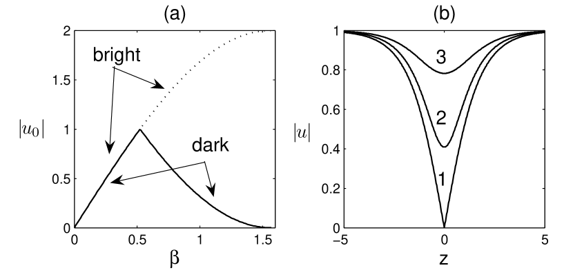
Figure 1: (a) Bright and dark soliton amplitudes versus the parameter $\beta$ for $\rho=1$. The dotted line and the solid line up to the bifurcation point correspond to the bright soliton. The solid line corresponds to the dark soliton. The bifurcation point is at $\beta_{cr}=\pi/6$ and $|u_{0}|=\rho$. (b) Dark soliton profiles for different $\beta$ and $\rho=1$. Curves $1$ (”black” soliton), $2$ and $3$ correspond to $\beta_{cr}=\pi/6$, $\beta=0.3$, and $\beta=1.1$, respectively.

As the first example, let us consider the simplest case when the function $a(\zeta)$ has one simple zero $\zeta_{1}$ in the first quadrant of the complex $\zeta$-plane on the $\rho$ circle (i. e. $M=1$, $N=0$) so that $\zeta_{1}=\rho\exp(i\beta_{1})$ with $0<\beta_{1}<\pi/2$. Taking into account Eq. (46), we have $b_{1}\exp(2ik_{1}x)=\epsilon\exp(-z)$, where $z=k_{0}(x-vt-x_{0})$ with

$$k_{0}=\rho^{2}\sin(2\beta_{1}),\qquad v=2\rho^{2}-\rho^{2}\cos(2\beta_{1}),$$ (55bp)

and without loss of generality one can set $\epsilon=\pm 1$. Determining $A_{12}^{(0)}$ and $A_{11}^{(0)}$ from (55bn) and solving a system of two linear algebraic equations for $A_{12}^{(1)}$ and $A_{11}^{(1)}$ from (55bd), (55be) we get

$$A_{12}^{(1)}=e^{-i\beta_{1}}\frac{(e^{3i\beta_{1}}-i\epsilon e^{-z})}{(e^{i\beta_{1}}+i\epsilon e^{-z})},\qquad A_{11}^{(1)}=\frac{(i+\epsilon e^{i\beta_{1}-z})}{\rho(e^{i\beta_{1}}+i\epsilon e^{-z})}$$ (55bq)

The one-soliton solution is $u(x,t)=iA_{12}^{(1)}/A_{22}^{(1)}$, and taking into account the property $A_{22}^{(j)}=A_{11}^{(j)\,\ast}$, we have

$$u(x,t)=\rho\left[1-\frac{2i\cos^{2}\beta_{1}}{\epsilon\sinh(z+i\beta_{1})+i}\right].$$ (55br)

The case $\epsilon=-1(1)$ corresponds to bright (dark) soliton. The parameters $k_{0}$ and $v$ in (55bp) are the soliton inverse width and the soliton velocity, respectively. In fact, there is only one parameter $\beta_{1}$ characterizing the soliton, and it is usually called a one-parametric soliton [5]. Amplitudes (with respect to the background) of the bright and dark solitons are $A_{b}=2\rho\sin\beta_{1}$ and $A_{d}=\rho-\rho|1-2\sin\beta_{1}|$, respectively. Dependences of the amplitudes on the parameter $\beta$ are shown in figure 1(a). It is interesting to note that the dark soliton amplitude is a nonmonotonic function of $\beta$ and the maximum occurs at $\beta_{cr}=\pi/6$. The dark soliton profiles $|u(z)|$ for different $\beta$ and $\rho=1$ are presented in figure 1(b). The dark soliton with $\beta=\beta_{cr}$ (the curve $1$ in figure 1(b)) may be called ”black” soliton: the intensity in the center of the soliton falls to zero. The corresponding one-soliton Jost solutions can easily be obtained from equations (43), (48) and (55bf)

$$\bar{\psi}_{1}(x,\zeta,t)=\frac{e^{-ik(\zeta)x}\zeta_{1}}{(\zeta^{2}-\zeta_{1}^{2})}[2\rho\sin\beta_{1}+(\zeta^{2}-\rho^{2})A_{11}^{(1)}]h(\zeta,t),$$ (55bs)

$$\psi_{1}(x,\zeta,t)=\frac{e^{ik(\zeta)x}\zeta_{1}^{\ast}}{\zeta(\zeta^{2}-\zeta_{1}^{\ast\,2})}[2i\rho^{2}\sin\beta_{1}+(\zeta^{2}-\rho^{2})A_{12}^{(1)}]h^{-1}(\zeta,t),$$ (55bt)

$$\varphi_{1}(x,\zeta,t)=\frac{e^{-ik(\zeta)x}\zeta_{1}^{\ast}}{(\zeta^{2}-\zeta_{1}^{\ast\,2})}[2\rho\sin\beta_{1}+(\zeta^{2}-\rho^{2})A_{11}^{(1)}]h(\zeta,t),$$ (55bu)

$$\bar{\varphi}_{1}(x,\zeta,t)=\frac{e^{ik(\zeta)x}\zeta_{1}}{\zeta(\zeta^{2}-\zeta_{1}^{2})}[2i\rho^{2}\sin\beta_{1}+(\zeta^{2}-\rho^{2})A_{12}^{(1)}]h^{-1}(\zeta,t).$$ (55bv)

The remaining Jost solutions can be found from the symmetry properties (23), (24) and (25)

$$\psi_{2}=\bar{\psi}_{1}^{\ast},\qquad\bar{\psi}_{2}=-\psi_{1}^{\ast},\qquad\bar{\varphi}_{2}=\varphi_{1}^{\ast},\qquad\varphi_{2}=-\bar{\varphi}_{1}^{\ast}.$$ (55bw)

Next we write out solutions for two more cases: the case when $a(\zeta)$ has two simple zeros in the first quadrant on the $\rho$ circle (i. e. $M=2$, $N=0$) so that

$$\zeta_{1}=\rho\exp(i\beta_{1}),\qquad\zeta_{2}=\rho\exp(i\beta_{2}),$$ (55bx)

and the case when $a(\zeta)$ has one simple zero in the first quadrant outside the $\rho$ circle (i. e. $M=0$, $N=1$)

$$\zeta_{1}=\rho\exp(\gamma_{1}+i\beta_{1}),\qquad\gamma_{1}>0.$$ (55by)

The case (55bx) corresponds to two-soliton solution for the one-parametric solitons, while the case (55by) corresponds to two-parametric one-soliton solution. In both cases we need to solve a system of four linear algebraic equations. Under this, the corresponding minors and determinants can be factorized and some parts of them are cancelled so that the resulting expressions for $u$ can significantly be simplified. The solutions are of the form

$$u=\rho\frac{BD}{D^{\ast\,2}},$$ (55bz)

where for the case (55bx)

$$B=1-i\epsilon_{1}e^{-3i\beta_{1}-z_{1}}-i\epsilon_{2}e^{-3i\beta_{2}-z_{2}}-\epsilon_{1}\epsilon_{2}\frac{\sin^{2}(\beta_{1}-\beta_{2})}{\sin^{2}(\beta_{1}+\beta_{2})}e^{-3i(\beta_{1}+\beta_{2})}e^{-z_{1}-z_{2}},$$ (55ca)

$$D=1-i\epsilon_{1}e^{i\beta_{1}-z_{1}}-i\epsilon_{2}e^{i\beta_{2}-z_{2}}-\epsilon_{1}\epsilon_{2}\frac{\sin^{2}(\beta_{1}-\beta_{2})}{\sin^{2}(\beta_{1}+\beta_{2})}e^{i(\beta_{1}+\beta_{2})}e^{-z_{1}-z_{2}},$$ (55cb)

where $z=k_{0,j}(x-v_{j}t-x_{0,j})$ ($j=1,2$) with

$$k_{0,j}=\rho^{2}\sin(2\beta_{j}),\qquad v_{j}=2\rho^{2}-\rho^{2}\cos(2\beta_{j}),$$ (55cc)

and, as before, $\epsilon_{j}=-1(1)$ corresponds to bright (dark) soliton. Equations (55bz), (55ca) and (55cb) describe collisions between bright/dark and bright/dark solitons.

For the case (55by) we get

$$B=\sinh 2\gamma_{1}\cosh(z+2\gamma_{1}+3i\beta_{1}-\ln\sinh 2\gamma_{1})+\sin 2\beta_{1}\sinh(3\gamma_{1}-i\varphi),$$ (55cd)

$$D=\sinh 2\gamma_{1}\cosh(z+2\gamma_{1}-i\beta_{1}-\ln\sinh 2\gamma_{1})-\sin 2\beta_{1}\sinh(\gamma_{1}+i\varphi),$$ (55ce)

with

$$z=k_{0}(x-vt-x_{0}),\qquad\varphi=\mu(x-wt)+\varphi_{0},$$ (55cf)

$$k_{0}=\rho^{2}\cosh 2\gamma_{1}\sin 2\beta_{1},\qquad\mu=\rho^{2}\sinh 2\gamma_{1}\cos 2\beta_{1},$$ (55cg)

$$v=2\rho^{2}-\rho^{2}\cos 2\beta_{1}\frac{\cosh 4\gamma_{1}}{\cosh 2\gamma_{1}},\qquad w=2\rho^{2}-\rho^{2}\cosh 2\gamma_{1}\frac{\cos 4\beta_{1}}{\cos 2\beta_{1}}.$$ (55ch)

The two-parametric soliton given by (55bz), (55cd) and (55ce) with the parameters $\gamma_{1}$ and $\beta_{1}$ is actually a breather (oscillating soliton) with period

$$T=\frac{2\pi}{\rho^{2}\tanh(2\gamma_{1})[\cosh^{2}(2\gamma_{1})+\cos^{2}(2\beta_{1})]},$$ (55ci)

and with velocity $v$ given by (55ch). If $\gamma_{1}\rightarrow 0$ and $\varphi_{0}\neq n\pi$ ($n$ is an integer), we have $T\rightarrow\infty$ and the breather reduces to the one-parametric soliton (bright or dark, depending on $\varphi_{0}$) given by (55br). The found soliton solutions perfectly coincide with those obtained in [15, 17].

4 Integrals of motion

Being completely integrable, the DNLSE with NVBC has an infinite set of integrals of motion. Eliminating $\varphi_{2}$ from (6), and substituting

$$\varphi_{1}=\exp\{-i\theta-ik(\zeta)x+i\eta^{-}(x)+q(x,\zeta)\},$$ (55cj)

into the resulting equation for $\varphi_{1}$, we get Riccati equation for the function $f=i(\rho^{2}-|u|^{2})/2+\partial_{x}q$

$$\partial_{x}f+(f-ik)^{2}-\frac{u^{\prime}}{u}(f-ik)+\lambda^{2}\left(|u|^{2}-i\frac{u^{\prime}}{u}+\lambda^{2}\right)=0,$$ (55ck)

where $u^{\prime}\equiv\partial_{x}u$. Representing

$$f(x,\zeta)=\frac{1}{i}\sum_{n=0}^{\infty}\frac{f_{n}(x)}{\zeta^{2n}},$$ (55cl)

and substituting (55cl) into (55ck), one can successively determine the coefficients $f_{n}(x)$. The first few of them are

$$f_{0}=\frac{1}{2}(|u|^{2}-\rho^{2}),$$ (55cm)

$$f_{1}=-iu\partial_{x}u^{\ast}-\frac{1}{2}(|u|^{4}-\rho^{4}),$$ (55cn)

$$f_{2}=2i(|u|^{2}-\rho^{2})u\partial_{x}u^{\ast}+i|u|^{2}u^{\ast}\partial_{x}u-2u\partial_{x}^{2}u^{\ast}+|u|^{4}(|u|^{2}-\rho^{2}).$$ (55co)

From equations (15) and (17) we have

$$\varphi_{1}\rightarrow e^{-i\theta-ikx},\qquad\mbox{as }x\rightarrow-\infty$$ (55cp)

$$\varphi_{1}\rightarrow ae^{i\theta-ikx}-\frac{i\rho}{\zeta}be^{i\theta+ikx},\qquad\mbox{as }x\rightarrow\infty.$$ (55cq)

It then follows from $\eta^{-}(-\infty)=0$ and from equation (55cj) that $q(-\infty,\zeta)=0$. Since $\eta^{-}(\infty)=\eta$, from equations (55cj) and (55cq) one can find that $q(\infty,\zeta)=\ln a(\zeta)+2i\theta-i\eta$ as $x\rightarrow\infty$ and $|\zeta|\rightarrow\infty$. On the other hand, from the definition of the function $f(x,\zeta)$ we have

$$q(\infty,\zeta)=\int_{-\infty}^{\infty}f(x,\zeta)\,dx-i\eta.$$ (55cr)

Thus, taking into account (55cl), one obtains

$$\ln a(\zeta)=-2i\theta-i\sum_{n=0}^{\infty}\frac{I_{n}}{\zeta^{2n}},$$ (55cs)

where

$$I_{n}=\int_{-\infty}^{\infty}f_{n}(x)\,dx$$ (55ct)

are integrals of motion. As usual, expanding (39) in power series with respect to $1/\zeta$ and using (55cs), one can explicitly express the integrals of motion in terms of discrete (solitonic) and continuous scattering data. In particular, for $I_{0}$ we get equation (40), and for $I_{1}$ we have

$$I_{1}=i\sum_{j=1}^{N}\left[\rho^{4}\left(\frac{1}{\zeta_{j}^{2}}-\frac{1}{\zeta_{j}^{\ast\,2}}\right)+(\zeta_{j}^{\ast\,2}-\zeta_{j}^{2})\right]+i\sum_{k=1}^{M}(\zeta_{k}^{\ast\,2}-\zeta_{k}^{2})$$

$$-\frac{1}{2\pi}\int_{\Gamma}\mu\ln(1-|b(\mu)|^{2})\,d\mu.$$ (55cu)

5 Perturbation theory

In the presence of perturbations the DNLSE can be written as

$$i\partial_{t}u+\partial_{x}^{2}u+i\partial_{x}(|u|^{2}u)=p[u,u^{\ast}],$$ (55cv)

where the perturbation is represented by the term $p[u,u^{\ast}]$. Equation (55cv) can be cast in the matrix form

$$\partial_{t}U-\partial_{x}V+[U,V]+P=0,$$ (55cw)

where

$$P=\left(\begin{array}[]{cc}0&i\lambda p\\ -i\lambda p^{\ast}&0\end{array}\right).$$ (55cx)

Then, evolution equation for the monodromy matrix $S$ can be obtained in a way similar to that described in [21]. As a result, we have

$$\partial_{t}S(t,\zeta)+i\Omega(\zeta)[\sigma_{3},S(t,\zeta)]=-\int_{-\infty}^{\infty}(M^{+})^{-1}(x,t,\zeta)PM^{-}(x,t,\zeta)dx.$$ (55cy)

The equations of motion for the coefficients $a(t,\zeta)$ and $b(t,\zeta)$ are contained in Eq. (55cy). Taking into account that $\det M^{\pm}=1+\rho^{2}/\zeta^{2}$ and equation (14), we have

$$\frac{\partial a}{\partial t}=\frac{i\zeta(\rho^{2}-\zeta^{2})}{(\rho^{2}+\zeta^{2})}\int_{-\infty}^{\infty}(p\psi_{2}\varphi_{2}+p^{\ast}\psi_{1}\varphi_{1})\,dx,$$ (55cz)

$$\frac{\partial b}{\partial t}-2i\Omega(\zeta)b=-\frac{i\zeta(\rho^{2}-\zeta^{2})}{(\rho^{2}+\zeta^{2})}\int_{-\infty}^{\infty}(p\bar{\psi_{2}}\varphi_{2}+p^{\ast}\bar{\psi_{1}}\varphi_{1})\,dx.$$ (55da)

The expression defining the zeros $\zeta_{j}(t)$ of $a(t,\zeta)$ is $a(t,\zeta_{j}(t))=0$. Differentiating with respect to $t$ gives

$$\partial_{t}a(t,\zeta_{j}(t))+\frac{\partial\zeta_{j}}{\partial t}\,a^{\prime}_{j}=0,$$ (55db)

where $a^{\prime}_{j}=da/d\zeta|_{\zeta=\zeta_{j}}$. Using (55cz) and (55db), one therefore finds

$$\frac{\partial\zeta_{j}}{\partial t}=-\frac{i\zeta_{j}(\rho^{2}-\zeta_{j}^{2})}{(\rho^{2}+\zeta_{j}^{2})a^{\prime}_{j}}\int_{-\infty}^{\infty}(p\psi_{2,j}\varphi_{2,j}+p^{\ast}\psi_{1,j}\varphi_{1,j})\,dx,$$ (55dc)

or, taking into account (29),

$$\frac{\partial\zeta_{j}}{\partial t}=-\frac{i\zeta_{j}(\rho^{2}-\zeta_{j}^{2})b_{j}}{(\rho^{2}+\zeta_{j}^{2})a^{\prime}_{j}}\int_{-\infty}^{\infty}(p\psi_{2,j}^{2}+p^{\ast}\psi_{1,j}^{2})\,dx,$$ (55dd)

where $\psi_{2,j}$, $\varphi_{2,j}$, $\psi_{1,j}$, and $\varphi_{1,j}$ are the corresponding Jost solutions evaluated at $\zeta=\zeta_{j}$. Evolution equation for $b_{j}$ can be obtained in a way similar to that described in Ref. [21]. As a result, one obtaines

$$\frac{\partial b_{j}}{\partial t}-2i\Omega(\zeta_{j})b_{j}=-\frac{i\zeta_{j}(\rho^{2}-\zeta_{j}^{2})}{(\rho^{2}+\zeta_{j}^{2})a^{\prime}_{j}}\int_{-\infty}^{\infty}\left\{p\,\varphi_{2}\frac{\partial}{\partial\zeta}\left(\varphi_{2}-b_{j}\psi_{2}\right)\right.$$

$$\left.+p^{\ast}\,\varphi_{1}\frac{\partial}{\partial\zeta}\left(\varphi_{1}-b_{j}\psi_{1}\right)\right\}dx^{\prime},$$ (55de)

where, after differentiating, the integrand is evaluated at $\zeta=\zeta_{j}$. Equations (55cz), (55da), (55dc) and (55de) describe the evolution of the scattering data.

If $p[u,u^{\ast}]$ is a small perturbation, one can substitute the unperturbed $N$-soliton Jost solutions $\psi$, $\bar{\psi}$, and $\varphi$ into the right-hand side of (55cz), (55da), (55dc) and (55de). This yields evolution equations for the scattering data in the lowest approximation of perturbation theory. This procedure can be iterated to yield higher orders of perturbation theory. The appearing hierarchy of equations is applied to an arbitrary number of solitons and, in particular, describes nontrivial many-soliton effects in the presence of perturbations. In this paper we restrict ourselves to the case of one-parametric one-soliton solutions with $\zeta_{1}=\rho\exp(i\beta_{1})$ and substitute unperturbed one-soliton Jost solutions (55bt)–(55bw) into the right-hand side of (55cz), (55da), (55dc) and (55de). The resulting equations are the desired set describing the evolution of the scattering data (both solitonic and continuous) in the presence of perturbations. Under this, equations (55dc) and (55de) corresponds to the so called adiabatic approximation, when an unperturbed instantaneous shape of one soliton with slowly varying parameters $\beta_{1}$ and $b_{1}$ is assumed, while equations (55cz) and (55da) account for radiative effects. Making use of the relation between the soliton solution (55br) and the corresponding squared Jost solution evaluated at $\beta_{1}$, the adiabatic equation for $\beta_{1}$ can be simplified to

$$\frac{\partial\beta_{1}}{\partial t}=\frac{i}{4}\int_{-\infty}^{\infty}(p^{\ast}u_{s}-pu_{s}^{\ast})\,dx,$$ (55df)

where $u_{s}$ is the one-parametric soliton solution (55br). Note, that this equation can also be obtained with the aid of the integral of motion $I_{0}$.

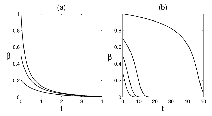
Figure 2: Dependence of the soliton parameter $\beta(t)$ on time for different initial $\beta(0)$ and for (a) bright and (b) dark solitons.

6 Application

As an example of using of the present perturbation theory, we consider the case when the perturbation term $p$ in (55cv) has the diffusive form

$$p=iD\frac{\partial^{2}u}{\partial x^{2}}.$$ (55dg)

This form of dissipative perturbation occurs for Alfvén solitons in a plasma when finite electric conductivity (and/or ion viscosity) of the plasma is taken into account [6, 21]. The conditions (in terms of the plasma parameters) under which the diffusive term (55dg) can be considered as a small perturbation are given in [6, 21]. We consider the action of perturbation on the one-parametric soliton (55br) in the adiabatic approximation. According to this approximation, the parameter $\beta$ of the soliton (55br) is considered as slowly varying in $t$ but with the unchanged functional shape. Then, substituting (55dg) into (55df) and calculating integrals with $u_{s}$ given by (55br), one can obtain

$$\frac{\partial\beta}{\partial t}=-4D\rho^{2}\sin\beta[\epsilon\sin\beta(\cos^{2}\beta-3)(\pi-2\epsilon\beta)+2\cos\beta(3-2\cos^{2}\beta)]$$ (55dh)

Numerically found solutions of (55dh) for different initial values of $\beta$ are shown in figures  2(a) and  2(b) for bright ($\epsilon=-1$) and dark ($\epsilon=1$) solitons respectively. For sufficiently small initial $\beta(0)\ll 1$, from (55dh) one can get a simple estimate $\beta(t)=\beta(0)\exp(-8D\rho^{2}t)$ both for bright and dark solitons, so that their amplitudes and velocities decrease with time. The situation, however, changes dramatically when $\beta(0)$ is not too small. Under this, the behaviour of bright and dark solitons is essentially different. First of all, as one can see in figure 2, dark solitons turn out to be much more robust. Next, if the initial $\beta$ exceeds the critical value $\beta_{cr}=\pi/6$ (see figure  1), then the amplitude $A_{d}$ (with respect to the background) of the dark soliton first increases with time, reaches a maximum for $\beta_{cr}=\pi/6$, where $A_{d}=\rho$, and finally decreases.

7 Conclusion

We have presented a simple approach for finding $N$-soliton solution and the corresponding Jost solutions of the DNLSE with NVBC. It is important that the exact solutions can be obtained without explicit determining of the phase factor. The found one- and two-soliton solutions perfectly coincide with those obtained in [15, 17], but, unlike [15, 17], our method allows to get solutions describing collisions between breathers, as well as collisions between pure bright/dark solitons and breathers.

We have also developed a perturbation theory based on the IST for perturbed DNLSE solitons. This approach fully uses the natural separation of the discrete and continuous degrees of freedom of the unperturbed DNLSE with NVBC. We have derived evolution equations for the scattering data (both solitonic and continuous) in the presence of perturbations. As an application of the developed theory, we considered (in the adiabatic approximation) the action of the diffusive-type perturbation on a single bright/dark soliton.

References

References

- [1] Rogister A 1971 Phys. Fluids 14 2733
- [2] Mjølhus E 1976 J. Plasma Phys. 16 321
- [3] Mio K et al1976 J. Phys. Soc. Japan 41 265
- [4] Mjølhus E and Wyller J 1986 Phys. Scr. 33 442
- [5] Mjølhus E 1989 Phys. Scr. 40 227
- [6] Mjølhus E and Wyller J 1988 J. Plasma Phys. 40 299
- [7] Kennel C F et al1988 Phys. Fluids 31 1949
- [8] Ruderman M S. 2002 J. Plasma Phys. 67 271
- [9] Ichikawa Y et al1980 J. Phys. Soc. Japan 48 279
- [10] Kaup D J and Newell A C 1978 J. Math. Phys. 19 798
- [11] Kawata T and Inoue H 1978 J. Phys. Soc. Japan 44 1968
- [12] Kawata T et al1979 J. Phys. Soc. Japan 46 1008
- [13] Kawata T et al1980 J. Phys. Soc. Japan 48 1371
- [14] Steudel H 2003 J. Phys. A: Math. Gen. 36 1931
- [15] Chen X J and Lam W K 2004 Phys. Rev. E 69 066604
- [16] Lashkin V M 2005 Phys. Rev. E 71 066613
- [17] Chen X J et al2006 J. Phys. A: Math. Gen. 39 3263
- [18] Chen X J et al2006 Phys. Lett. A 353 185
- [19] Wyller J and Mjølhus E 1984 Physica D 13 234
- [20] Faddeev L D and Takhtajan L A 1987 Hamiltonian Methods in the Theory of Solitons (Berlin: Springer-Verlag)
- [21] Lashkin V M 2006 Phys. Rev. E 74 016603