Two-dimensional nonlocal vortices, multipole solitons and azimuthons in dipolar Bose-Einstein condensates.

Abstract

We have performed numerical analysis of the two-dimensional (2D) soliton solutions in Bose-Einstein condensates with nonlocal dipole-dipole interactions. For the modified 2D Gross -Pitaevski equation with nonlocal and attractive local terms, we have found numerically different types of nonlinear localized structures such as fundamental solitons, radially symmetric vortices, nonrotating multisolitons (dipoles and quadrupoles), and rotating multisolitons (azimuthons). By direct numerical simulations we show that these structures can be made stable.

I Introduction

The recent first experimental realization of a degenerate dipolar atom gas Exper1 , where a Bose-Einstein condensate (BEC) of ⁵²Cr atoms has been observed, and optimistic perspectives in creating a degenerate gas of polar molecules Exper2 have stimulated a growing interest in the study of BEC with nonlocal dipole-dipole interactions Santos05 ; Pedri06 ; Lushnikov . Dipole-dipole forces are anisotropic and long range, so that the inter-particle interaction becomes essentially nonlocal.

Nonlocal nonlinearity naturally arises in many areas of nonlinear physics and plays a crucial role in the dynamics of nonlinear coherent structures. In particular, a rigorous proof of absence of collapse in arbitrary spatial dimensions during the wave-packet propagation described by the nonlocal nonlinear Schrödinger equation (NLSE) with sufficiently general symmetric response kernel has been presented in Refs. Tur ; Krol . Stable vortex Yakimenko ; Briedis , dipole We1 ; Lopez ; Skupin ; Kartashov and azimuthon Lopez ; Skupin ; We2 solitons in media with nonlocal nonlinear response were theoretically predicted. Finally, nonlocality induces attraction between solitons and allows for the formation of bound states of out-of-phase bright solitons Mironov and dark solitons Nikolov .

A very attractive feature of BEC with dipole-dipole interactions is that the interplay between the nonlocal interaction, which is only partially attractive and may be tuned by means of rotating orienting fields Tune , and the usual local short-range contact forces, leads to the possibility of experimental realization of highly controllable and stable solitary structures in BEC Santos05 .

Recently, Pedro and Santos Santos05 have studied the physics of bright solitons in two-dimensional (2D) dipolar Bose-Einstein condensates with repulsive short-range interactioins. Using the reduction procedure, they have obtained 2D modified Gross -Pitaevski equation with the nonlocal term describing dipole-dipole interaction and showed that the existence of stable 2D solitary waves is possible.

In this paper, using 2D model suggested by Pedri and Santos Santos05 , we study 2D solitary waves (SWs) in BEC with attractive short-range and nonlocal dipole-dipole interactions. As is known, the collapse of BEC s at some critical number of atoms is the main consequence of the attractive nonlinearity Dalfovo . The presence of nonlocal interaction, however, significantly changes the situation and leads to stable localized states. We present different types of SWs (fundamental solitons, vortices, nonrotating and rotating multisolitons) and by direct numerical simulations show that these localized structures can be made stable.

II Model and basic equations

A dipolar BEC, consisting of $\mathcal{N}$ particles with the dipole moment $d$ oriented along the $z$-axis, at sufficiently low temperatures is described by a NLSE with nonlocal nonlinearity

$$i\hbar\frac{\partial\Psi}{\partial t}=\left[-\frac{\hbar^{2}}{2m}\Delta+U(\mathbf{r})+g|\Psi|^{2}\right.$$

$$\left.+\int V(\mathbf{r}-\mathbf{r^{\prime}})|\Psi(\mathbf{r^{\prime}})|^{2}\,d\mathbf{r^{\prime}}\right]\Psi,$$ (1)

where $\Psi(\mathbf{r},t)$ is the condensate wave function normalized to the total number of particles: $\int|\Psi(\mathbf{r})|^{2}\,d\mathbf{r}=\mathcal{N}$. The coupling constant $g$ corresponds to the local contact interaction and $g=4\pi\hbar^{2}a/m$, where $a$ is the $s$-wave scattering length. In the following, we consider $a<0$, i.e. attractive short-range interactions. An external trapping potential is assumed to be of the form $U(\mathbf{r})=m\omega_{z}^{2}z^{2}/2$, with no trapping in the $xy$-plane. All dipoles are assumed to be oriented along the trap axis. The nonlocal potential is due to the dipole-dipole interaction, and the kernel $V(\mathbf{r})$ is given by $V(\mathbf{r})=g_{d}(1-3\cos^{2}\theta)/r^{3}$, where $g_{d}=\alpha\mu_{0}d^{2}/4\pi$, $\theta$ is the angle between the vector $\mathbf{r}$ and the dipole axis, $\mu_{0}$ is the magnetic permeability of the vacuum, and $-1/2\leq\alpha\leq 1$ is a tunable parameter Santos05 ; Tune .

Assuming the anzatz $\Psi(\mathbf{r})=\psi(\mathbf{r}_{\perp})\varphi_{0}(z)$, where the function $\varphi_{0}(z)$, describing the condensate in the direction of the tight confinement, is the ground state of the 1D harmonic oscillator in the $z$-direction and normalizing the length, time, and wave function by $l_{z}/\sqrt{2}$, $1/\omega_{z}$, and $(\mathcal{N}/l_{z}^{3})^{1/2}$, respectively (where $l_{z}=(\hbar/m\omega_{z})^{1/2}$), authors of Ref. Santos05 , following the standard reduction procedure, obtained the following 2D equation

$$i\frac{\partial\psi}{\partial t}=-\Delta_{\perp}\psi+\bar{g}\psi\left\{|\psi|^{2}+\beta\int R(\mathbf{r}-\mathbf{r}^{\prime})|\psi(\mathbf{r}^{\prime})|^{2}\,d\mathbf{r}^{\prime}\right\},$$ (2)

with the two free dimensionless parameters

$$\bar{g}=\frac{g}{\sqrt{2\pi}\hbar\omega_{z}l_{z}^{3}}=\frac{2\sqrt{2\pi}a}{l_{z}},\quad\beta=\frac{g_{d}}{g}.$$ (3)

The Fourier transform of the kernel $R(\mathbf{r})$ in Eq. (2) is

$$\hat{R}(\mathbf{k})=2-3\sqrt{\pi}ke^{k^{2}}\mathop{\rm erfc}\nolimits(k),$$ (4)

where $\mathop{\rm erfc}\nolimits(x)$ is the complementary error function, so that

$$R(\mathbf{r})=\frac{1}{(2\pi)^{2}}\int e^{i\mathbf{k}\cdot\mathbf{r}}\hat{R}(\mathbf{k})\,d\mathbf{k}.$$ (5)

In what follows, since Eq. (2) admits an additional rescaling, the parameter $\bar{g}$ has been fixed at $\bar{g}=\mp 1$, where the $-$($+$) sign corresponds to attractive (repulsive) short-range interaction.

Equation (2) conserves the 2D norm, $N=\int|\psi|^{2}dxdy$, and energy

$$E=\int\left\{\left|\frac{\partial\psi}{\partial x}\right|^{2}+\left|\frac{\partial\psi}{\partial y}\right|^{2}+\frac{1}{2}\bar{g}|\psi|^{4}+\frac{1}{2}\bar{g}\beta|\psi|^{2}\right.$$

$$\times\left.\left[\int R(\mathbf{r}-\mathbf{r}^{\prime})|\psi(\mathbf{r}^{\prime})|^{2}\,d\mathbf{r}^{\prime}\right]\right\}dxdy.$$ (6)

III Modulational instability

An important feature of the dipole-dipole interaction is that, due to the anisotropy, it is only partially attractive. Correspondingly, the spectrum $\hat{R}(k)$ of the response function $R(\mathbf{r})$ is not sign definite (note, in this connection, that an analysis of 2D soliton dynamics in the framework of Eq. (2) with somewhat resembling Eq. (4), but positive definite, kernel $\hat{R}(k)$ was performed in Ref. Skupin ). Equation (2) has a solution in the form of plane wave

$$\Psi_{0}=|\Psi_{0}|\exp(i\mathbf{k}_{0}\cdot\mathbf{r}-i\omega t)$$ (7)

provided $\omega=k_{0}^{2}-\bar{g}(1+\beta\int R(\mathbf{r})d\mathbf{r})|\Psi_{0}|^{2}$. The stability properties of the plane wave essentially depend on sign definiteness of the spectrum of nonlinear response function Krol ; Wyller . On the other hand, modulational instability (MI) (instability of the plane wave with amplification of both sidebands) is often considered as a precursor for the formation of bright solitons. Considering perturbed plane wave solutions in the form

$$\psi=(|\Psi_{0}|+\delta\psi)\exp(i\mathbf{k}_{0}\cdot\mathbf{r}-i\omega t),$$ (8)

where

$$\delta\psi=\psi_{+}e^{i\mathbf{k}\cdot\mathbf{r}-\gamma t}+\psi_{-}e^{-i\mathbf{k}\cdot\mathbf{r}+\gamma t},$$ (9)

and linearizing Eq. (2) around $\Psi_{0}$ in $\delta\psi$, one can obtain the growth rate $\gamma$ of MI of homogeneous field ($k_{0}=0$) for the model Eq. (2)

$$\gamma^{2}=-2|\Psi_{0}|^{2}k^{2}\bar{g}[1+\beta\hat{R}(k)]-k^{4}.$$ (10)

Instability occurs if $\gamma^{2}>0$. In Figure  1 we show the dependence of the growth rate of MI on $k$ for the cases of attractive ($\bar{g}=-1$) and repulsive ($\bar{g}=1$) short-range interactions. In the attractive case, the growth rate is equal to zero for $0\leq k<k_{cr}$, where $k_{cr}$ is some critical value depending on $\beta$ (the ratio between dipole-dipole and short-range interaction), if $\beta\lesssim 0.5$ (i. e., in particular, for all negative $\beta$), so that long wave modes are stable. Optimal, i.e. corresponding to maximum of the growth rate, wave number $k_{opt}$ decreases with increasing $\beta$. In the repulsive case, the growth rate of MI is equal to zero for all positive $\beta$ and for $\beta\gtrsim-0.4$. This is in agreement with results of Ref. Santos05 , where bright solitons (for the repulsive case $\bar{g}=1$) were predicted only for negative $\beta$ and $|\beta|>0.12$.

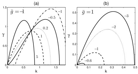
Figure 1: The growth rates $\gamma$ of the modulational instability for (a) attractive ($\bar{g}=-1$) and (b) repulsive ($\bar{g}=1$) short-range interactions. Values of $\beta$ (the ratio between dipole-dipole and short-range interaction) are shown near the curves.

IV Numerical results

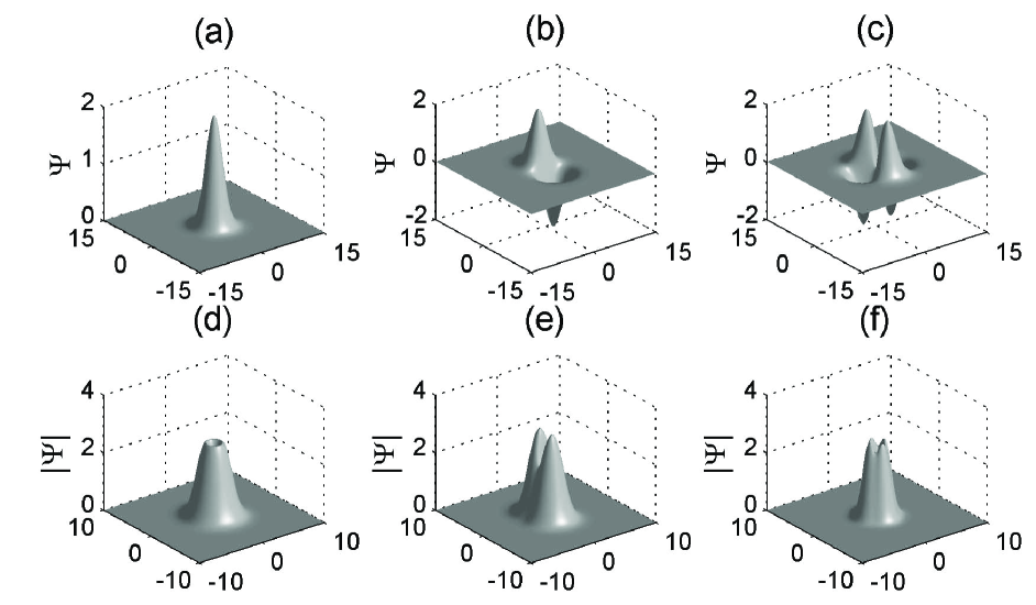
Figure 2: Numerically found stationary localized nonrotating (a-c) and rotating (d-f) solutions of Eq. (2) with $\beta=2$: (a) monopole with $\mu=-2$; (b) dipole with $\mu=-2$; (c) quadrupole with $\mu=-2$; (d) vortex with $\mu=-5$; (e) azimuthon with $\mu=-5$, $p=0.6$ and two intensity peaks; (f) azimuthon with $\mu=-5$, $p=0.9$ and four intensity peaks.

We look for stationary solutions of Eq. (2) with $\bar{g}=-1$ (attractive short-range interaction) in the form $\psi(x,y,t)=\Psi(x,y)\exp(-i\mu t)$, where $\mu$ is the chemical potential, so that $\Psi$ obeys the equation

$$(\mu+\Delta_{\perp})\Psi=-\Psi\left\{|\Psi|^{2}+\beta\int R(\mathbf{r}-\mathbf{r}^{\prime})|\Psi(\mathbf{r}^{\prime})|^{2}\,d\mathbf{r}^{\prime}\right\},$$ (11)

where $R(\mathbf{r})$ is determined by Eqs. (4) and (5). To solve numerically Eq. (11), we impose periodic boundary conditions on Cartesian grid and use the relaxation technique similar to one described in Ref. Petviashvili . We have not found any localized solutions with $\mu>0$. Fundamental soliton solutions of Eq. (11) with $\beta<0$ or $\beta>\beta_{cr}$, where $\beta_{cr}\sim 2.1$, turn out to be unstable with $\partial N/\partial\mu>0$. Thus, in what follows, we consider the region $0<\beta<\beta_{cr}$ and specifically set $\beta=2$. Choosing an appropriate initial guess, one can find numerically with high accuracy (the norms of the residuals were less than $10^{-9}$) three different classes of spatially localized solutions of Eqs. (11) – the nonrotating (multi)solitons, the radially symmetric vortices, and the rotating multisolitons (azimuthons).

The real (or containing only a constant complex factor) function $\Psi(x,y)$ corresponds to nonrotating solitary structures. Examples of such nonrotating (multi)solitons for Eq. (11), namely, a monopole, a dipole, and a quadrupole are presented in Figs. 2(a)- 2(c). The nonrotating multipoles consist of several fundamental solitons (monopoles) with opposite phases.

The second class of solutions, vortex solutions, are the solutions with the radially symmetric amplitude $|\Psi(x,y)|$, that vanishes at the center, and a rotating spiral phase in the form of a linear function of the polar angle $\theta$, i.e. $\arg\Psi=m\theta$, where $m$ is an integer. The index $m$ (topological charge) stands for a phase twist around the intensity ring. The important integral of motion associated with this type of solitary wave is the angular momentum, which can be expressed through the vortex amplitude and phase. The numerically found single-charged ($m=1$) vortex solution of Eq. (11) is shown in Fig. 2(d).

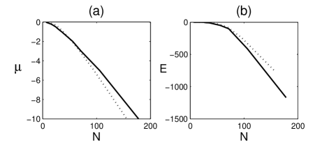
Figure 3: (a) Chemical potential $\mu$ and (b) energy $E$ versus normalized number of atoms $N$. Solid line: nonrotating dipoles ($p=0$). Dotted line: vortices ($p=1$).

The third class of solutions, rotating multisolitons with the spatially modulated phase, were first introduced in Ref. Kivshar1 for models with local nonlinearity, where they were called azimuthons. The azimuthons can be viewed as an intermediate kind of solutions between the rotating radially symmetric vortices and nonrotating multisolitons. Using variational analysis to describe azimuthons, the authors of Ref. Lopez considered the following trial function in polar coordinates ($r$,$\theta$)

$$\Psi(r,\theta)=r^{|m|}\Phi(r)(\cos m\theta+ip\,\sin m\theta),$$ (12)

where $\Phi$ is the real function, which vanish fast enough at infinity, $m$ is an integer, and $0\leq p\leq 1$. The case $p=0$ corresponds to the nonrotating multisolitons (e. g. $m=1$ to a dipole, $m=2$ to a quadrupole etc.), while the opposite case $p=1$ corresponds to the radially symmetric vortices. The intermediate case $0<p<1$ corresponds to the azimuthons. In our case, the numerically found complex function $\Psi(x,y)$ with a spatially modulated phase corresponds to the azimuthons. We introduced the parameter $p$ (modulational depth), which is similar to the one in Eq. (12), in the following way

$$p=\max|\mathrm{Im}\,\Psi|/\max|\mathrm{Re}\,\Psi|.$$ (13)

For fixed chemical potential $\mu$, there is a family of azimuthons with different $p$. Like the radially symmetric vortices, the azimuthons carry out the nonzero angular momentum. In Figures 2(e) and  2(f) we demonstrate two numerically found examples of the azimuthons for the nonlocal model described by Eqs. (2). Figure  3 shows the dependences of the chemical potential $\mu$ and energy $E$ on the normalized number of atoms $N$, for the dipoles ($p=0$) and vortices ($p=1$).

We next addressed the stability of these localized solutions and study the evolution of the solitons in the presence of small initial perturbations. We have undertaken extensive numerical modeling of Eq. (2) initialized with our computed solutions with added gaussian noise. The initial condition was taken in the form $\Psi(x,y)[1+\varepsilon\Phi(x,y)]$, where $\Psi(x,y)$ is the numerically calculated exact solution, $\Phi(x,y)$ is the white gaussian noise with variance $\sigma^{2}=1$ and the parameter of perturbation $\varepsilon=0.005\div 0.1$. In addition, azimuthal perturbation of the form $i\varepsilon\sin\theta$ was taken for the vortices and azimuthons. Spatial discretization was based on the pseudospectral method. Under this, since the Fourier transform of the kernel $R$ is known, the nonlocal term can be easily computed with the aid of the convolution theorem. Temporal $t$-discretization included the split-step scheme. As was said above, we consider the region $0<\beta<\beta_{cr}$.

The fundamental solitons are stable for all $\mu<0$. These solitons have $\partial N/\partial\mu<0$ so that the Vakhitov-Kolokolov stability criterion is met.

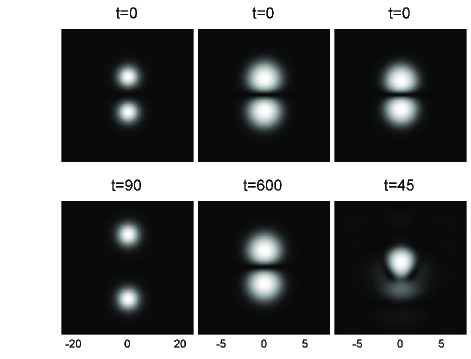
Figure 4: Left column: Splitting of the dipole with $\mu=-0.2$ into two monopoles; middle column: stable dynamics of the dipole with $\mu=-3$; right column: unstable dipole with $\mu=-4$.

Depending on the parameter $\mu$, we observed three different scenarios of the nonrotating dipole evolution, which are presented in Fig. 4 (for $\varepsilon=0.01$). The first regime corresponds to the region $\mu_{cr}<\mu<0$, and for $\beta=2$ we found $\mu_{cr}\sim-0.2$, which corresponds to the normalized number of atoms $N_{cr}\sim 15.5$. If $\mu_{cr}<\mu$, the initial dipole splits in two monopoles which move in the opposite directions without changing their shape and without radiation, i. e. the monopoles just go away at infinity. This type of the evolution is shown in the left column of Fig. 4. Under this, the value $\delta N=N_{dip}-2N_{mon}$, where $N_{dip}$ and $N_{mon}$ are 2D norms for the dipole and monopole respectively, tends to almost zero as $\mu$ approaches $\mu_{cr}$.

The second regime of the dipole evolution corresponds to the region $\mu_{th}<\mu<\mu_{cr}$, where (for $\beta=2$) $\mu_{th}\sim-3.1$. The numerical simulations clearly show that in this range of the parameter $\mu$ the dipoles are stable with respect to initial noisy perturbations and survive over huge times. In terms of the 2D norm (normalized number of atoms), the stability region is written as $N_{cr}<N<N_{th}$, where $N_{th}\sim 71$. The stable dynamics of the dipole is illustrated in the middle column of Fig. 4 (for $\beta=2$, $\mu=-3$ and $\varepsilon=0.01$).

The further (after $\mu_{th}\sim-3.1$) decreasing of the chemical potential $\mu$ (or, equivalently, increasing of the normalized number of atoms $N$) sharply shortens the times at which the dipole survives, and, the dipoles with $\mu<\mu_{th}$ are unstable. The typical decay of the unstable dipole below the threshold value $\mu_{th}$ of the chemical potential is shown in the right column of Fig. 4. Thus, the stable dipoles exist only within a finite, rather narrow range of the normalized number of atoms $N$.

A somewhat different behavior we observed for the vortices. The numerical simulations clearly show that the vortices with $\mu<\mu_{cr}$, where $\mu_{cr}$ is some critical value and for $\beta=2$ we found $\mu_{cr}\sim-1.4$ (with corresponding $N_{cr}\sim 45$), are stable with respect to small initial noisy and azimuthal perturbations up to the maximum times used (of the order of $t=1000$). The vortices with $\mu>\mu_{cr}$ (i.e. $N<N_{cr}$) splits in two fundamental solitons moving in the opposite directions. These two different scenarios of the vortex evolution are illustrated in Fig. 5. Thus, the vortices can be made stable if the 2D norm (normalized number of atoms) exceeds some critical value $N_{cr}$.

We have not performed numerical analysis of the azimuthon evolution for different $\lambda$ and arbitrary $p$ because of the difficulties in finding azimuthon solutions with arbitrary $p$. Nevertheless, we can conclude that azimuthons with two intensity peaks and not too small $p$ can be made stable if the 2D norm (normalized number of atoms) $N$ exceeds some critical value depending on $p$. Splitting of the azimuthon with two intensity peaks and $\mu=-1$, $p=0.4$, and stable dynamics of the azimuthon with $\mu=-5$ and $p=0.6$ are shown in Fig. 6. Numerically estimated rotational velocity of the stable azimuthon in Fig. 6(b) is $\omega=0.18$ so that it survives over many dozens of rotational periods.

Note, that one point should be emphasized. Strictly speaking, our direct numerical modelling can not give a rigorous proof of stability/instability of the multisolitons. First, in the the direct numerical experiments one can consider the evolution over finite times only. Second, the results are limited to the perturbation profile. A rigorous proof could, for instance, include a linear stability analysis with the corresponding eigenvalue problem. Nevertheless, from our numerical simulations of the dynamics over finite, but large, times we can conclude that (in stable cases) the potential growth rates of unstable modes are very small. The structures (if stable) survive over huge times and hundreds of rotational periods, and from the practical point of view they can be regarded as stable.

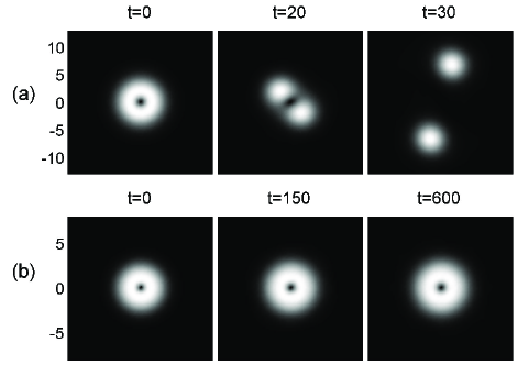
Figure 5: (a) Splitting of the vortex with $\mu=-1$; (b) stable dynamics of the vortex with $\mu=-5$.

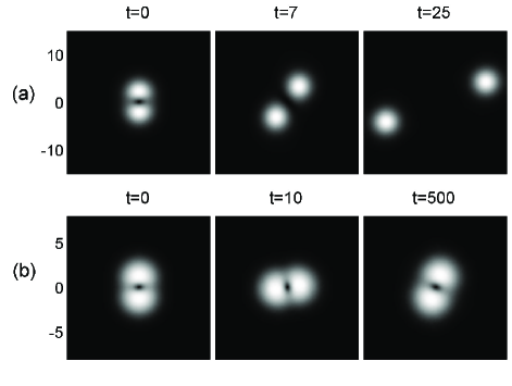
Figure 6: (a) Splitting of the azimuthon with two intensity peaks and $\mu=-1$, $p=0.4$; (b) stable dynamics of the azimuthon with two intensity peaks and $\mu=-5$, $p=0.6$.

V Conclusion

In conclusion, we have demonstrated the existence of 2D localized nonlinear structures in BECs with nonlocal dipole-dipole and attractive short-range contact interactions and studied their stability. We have found numerically three kinds of soliton families: nonrotating multipole solitons (fundamental one-hump soliton, dipole and quadrupole), radially symmetric vortices, and rotating multihump (with two and four intensity peaks) solitons with the spatially modulated phase (azimuthons). We have shown that stable solitons may exist only within a finite range of the ratio between dipole-dipole and short-range interactions (both of which are tunable). The anisotropy of the dipole-dipole interaction is crucial, since this leads to partially attractive nature of the interaction. Sufficiently large dipolar interactions destabilize the SWs. By direct numerical simulations, we have found that dipole nonrotating solitons, vortices and two intensity peak azimuthons can be stable for some values of the chemical potential (or, equivalently, normalized number of atoms).

- (1) A. Griesmaier et al., Phys. Rev. Lett. 94, 160401 (2005).
- (2) D. J. M. Sage et al., Phys. Rev. Lett. 94, 203001 (2005).
- (3) P. Pedri and L. Santos, Phys. Rev. Lett. 95, 200404 (2005).
- (4) R. Nath, P. Pedri and L. Santos, cond-mat/0610703.
- (5) P. M. Lushnikov, Phys. Rev. A 66, 051601(R) (2002).
- (6) S.K. Turitsyn, Theor. Math. Phys. 64, 797 (1985).
- (7) W. Krolikowski, O. Bang, N. I. Nikolov, D. Neshev, J. Wyller, J. J. Rasmussen, and D. Edmundson, J. Opt. B 6, S288 (2004).
- (8) A. I. Yakimenko, Yu. A. Zaliznyak, and Yu. Kivshar Phys. Rev. E. 71, 065603 (2005)
- (9) D. Briedis, D. E. Petersen, D. Edmundson, W. Krolikowski, and O. Bang, Opt. Express 13, 435 (2005).
- (10) A. I. Yakimenko, V. M. Lashkin, and O. O. Prikhodko, Phys. Rev. E 73, 066605 (2006).
- (11) Y.V. Kartashov, L. Torner, V. A. Vysloukh, and D. Mihalache, Opt. Lett. 31, 1483 (2006).
- (12) S. Lopez-Aguayo et al., Opt. Lett. 31, 1100 (2006).
- (13) S. Skupin, O. Bang, D. Edmundson, and W. Krolikowski, Phys. Rev. E 73, 066603 (2006).
- (14) V. M. Lashkin, A. I. Yakimenko, and O. O. Prikhodko, nlin.PS/0607062.
- (15) I. A. Kolchugina, V. A. Mironov, and A. M. Sergeev, JETP Lett. 31, 304 (1980).
- (16) N. I. Nikolov et al., Opt. Lett. 29, 286 (2004).
- (17) S. Giovanazzi, A. Görlitz, and T. Pfau, Phys. Rev. Lett. 89, 130401 (2002).
- (18) F. Dalfovo, S. Giorgini, L. P. Pitaevskii, and S. Stringari, Rev. Mod. Phys. 71, 463 (1999).
- (19) J. Wyller et. al., Phys. Rev. E 66, 066615 (2003).
- (20) A. S. Desyatnikov, A. A. Sukhorukov, and Yu. S. Kivshar, Phys. Rev. Lett. 95, 203904 (2005) .
- (21) V.I. Petviashvili and V.V. Yan’kov, in Reviews of Plasma Physics, edited by B. B. Kadomtsev, (Consultants Bureau, New York, 1989), Vol. 14.