Growing condensate in two-dimensional turbulence

Abstract

We report a numerical study, supplemented by phenomenological explanations, of “energy condensation” in forced 2D turbulence in a biperiodic box. Condensation is a finite size effect which occurs after the standard inverse cascade reaches the size of the system. It leads to emergence of a coherent vortex dipole. We show that the time growth of the dipole is self-similar, and it contains most of the injected energy, thus resulting in an energy spectrum which is markedly steeper than the standard $k^{-5/3}$ one. Once the coherent component is subtracted, however, the remaining fluctuations have a spectrum close to $k^{-1}$. The fluctuations decay slowly as the coherent part grows.

A big difference between 2D and 3D turbulence is the generation of large scale structures from small scale motions Frisch (1995); Kellay and Goldburg (2002). This occurs because, if pumped at intermediate scales, the 2D Navier–Stokes equations favor energy transfer to larger scales Kraichnan (1967); Leith (1968); Batchelor (1969); Chen et al. (2006), a phenomenon known as an inverse cascade. Simulations Smith and Yakhot (1993, 1994) and experiments Paret and Tabeling (1998); Jin and Dubin (2000); Shats et al. (2005) show that large scale accumulation of energy is observed if conditions permit the energy to reach the system size. In this letter, we study the “condensate” emerging in the form of two coherent vortices in a biperiodic box in 2D. Let us begin by briefly reviewing the classical 2D turbulence theory of Kraichnan, Leith and Batchelor (KLB) Kraichnan (1967); Leith (1968); Batchelor (1969). The essential difference with 3D turbulence is the presence of a second inviscid invariant, in addition to energy, the enstrophy. Stirring the 2D flow leads to emergence of two cascades. Enstrophy cascades from the forcing scale, $l$, to smaller scales (direct cascade) while energy cascades from the forcing scale to larger scales (inverse cascade). Viscosity dissipates enstrophy at the Kolmogorov scale, $\eta$, which is much smaller than $l$ when the Reynolds number is large. The energy cascade is blocked at a scale $\zeta$, $\zeta\gg l$, by a frictional dissipation (usually due to friction between the fluid and substrate although other mechanisms can be imagined) after a transient in time quasi-stationary regime. Then a stationary KLB turbulence is established Kraichnan (1967); Leith (1968); Batchelor (1969). Applying Kolmogorov phenomenology (see e.g. Frisch (1995)) KLB predicts an energy spectrum scaling as $k^{-3}$ in the direct cascade, and as $k^{-5/3}$ in the inverse cascade. Here $k$ is the modulus of the wave-vector. The KLB spectra imply that velocity fluctuations at a scale $r$, $\delta v_{r}$ scale as $\epsilon^{1/3}l^{-2/3}r$ and $(\epsilon r)^{1/3}$ in the direct and inverse cascade ranges respectively. KLB theory is confirmed by simulations Boffetta et al. (2000); Boffetta (2006) and experiments Bruneau and Kellay (2005); Kellay and Goldburg (2002), where a sufficient range of scales was available to form the cascades. If the frictional dissipation is weak so that $\zeta$ exceeds the system size $L$ then ultimately the “condensate” regime emerges Kraichnan (1967); Smith and Yakhot (1993) where the standard KLB does not apply.

One of the primary motivations for studying 2D turbulence is that it is structurally and phenomenologically similar to quasi-geostrophic turbulence Lesieur (1997); Charney (1971) which describes planetary atmospheres Nastrom and Gage (1985). In addition, a recent resurgence in theoretical interest in the condensate state was sparked by experimental Shats et al. (2005) and numerical Molenaar et al. (2004) observations of large scale coherent vortices associated with energy condensation in forced, bounded flows. In this letter, we report results of a set of numerical experiments designed to give a clean, detailed study of this energy condensation phenomenon in its own right.

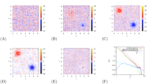
Figure 1: Vorticity snapshots at a succession of times : (A) $t=100$, (B) $t=2000$, (C) $t=10000$. Decomposition of the $t=10000$ snapshot into coherent, (D), and fluctuating parts, (E). Energy spectra of the full field, coherent part and fluctuating part, (F).

We solved the incompressible forced Navier–Stokes equations with hyperviscous dissipation in 2D:

$$\partial_{t}{\bm{u}}+({\bm{u}\cdot\nabla}){\bm{u}}+{\bm{\nabla}}p = \nu\Delta^{8}{\bm{u}}+{\bm{f}}$$

$${\bm{\nabla}}\cdot{\bm{u}} = 0.$$ (1)

The domain is a doubly-periodic box of size, $L=2\pi$. The forcing, ${\bm{f}}$, injects velocity fluctuations and energy at an intermediate scale $l$ with energy injection rate $\epsilon$. For the simulations shown in Figs. 1 and  3, $l=2\pi/50$ and $\epsilon=0.004$. We use a standard pseudo-spectral solver with full dealiasing. The resolution varied from $256^{2}$ to $1024^{2}$. For developed condensate computations, the resolution was only $256^{2}$ owing to the requirement of integration for tens of thousands of forcing times, which was done using a 3rd order Runge–Kutta integrator with integrating factors. The timestep was decreased as the condensate grows such that it satisfies $\Delta t<c_{0}\Delta x/u_{\rm max}$, where $\Delta x$ is the grid spacing, $u_{\rm max}$ is the maximum velocity and $c_{0}$ is conservatively taken in the range $0.2$ – $0.5$. Energy injection was done in a spectral band using a stochastic additive force with fixed amplitude and random phase. The correlation time is the numerical timestep. Small scale dissipation was provided by $\Delta^{8}$ hyperviscosity which is not expected to affect the large scale behavior. There is evidence Danilov and Gurarie (2001), and our additional simulations (not discussed here) are in support, that the presence of large scale damping can considerably complicate the description of the large scales.

The forcing described above is short correlated in time and characterized by the energy injection rate, $\epsilon$, and the forcing scale, $l$. The majority of the injected enstrophy cascades towards smaller scales to be dissipated by viscosity. In our numerics, the closeness of $\eta$ to $l$ meant that only 40% of the injected energy goes upscale from $l$ with the rest going downscale with the enstrophy. We simulate the zero friction case to assure that eventually the energy starts piling up at the system size scale. The direct cascade is set up in a short time, $\tau_{l}\sim l^{2/3}/\epsilon^{1/3}$. The time, $\tau_{*}$, for the inverse cascade to populate all scales up to $L$, is much longer. Based on Kolmogorov arguments, $\tau_{*}\sim\epsilon^{-1/3}L^{2/3}$. In the simulations, $\tau_{*}\approx 1000$, in units where $\tau_{l}$ is about 1.

At $t>\tau_{*}$ we observed a condensate consisting of two big vortices of the size $\sim L$ separated by a hyperbolic domain of comparable size. Fig. 1 (A),(B) and (C) illustrates the phenomenon with a series of vorticity snapshots. The condensate is formed to ensure that (a) the integral vorticity is zero in accordance with zero integral vorticity injected by the small-scale pumping, and (b) majority of energy brought by the inverse cascade is accumulated at the largest scale, $L$. Two identical vortices rotating in opposite directions satisfy these conditions. Due to biperiodicity, Fig. 1 actually depicts the emergence of a vortex crystal. Such crystals have been observed both numerically Smith and Yakhot (1994) and experimentally Jin and Dubin (2000). The vortices drift slowly over time but the square symmetry of the crystal is preserved by this drift.

Evolution of the vortices is slow relative to the background fluctuations which permits a separation of the flow into coherent and fluctuating components in the spirit of Farge and Rabreau (1988); Farge et al. (1999). The highest amplitude coefficients of the wavelet transformed vorticity are assigned to the coherent component and the remainder to the incoherent component. Inverse wavelet transforms are then taken. This decomposition is shown in Fig. 1 (D) and (E). Fig. 1(E) shows that the fluctuating part is almost statistically homogeneous, whereas the coherent part is strongly inhomogeneous. Note that the characteristic amplitude of the vorticity fluctuations is larger than the coherent part of the vorticity over most of the domain. Ultimately we expect the coherent flow to dominate the fluctuations everywhere but we have not reached this regime.

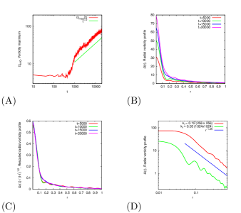
Figure 2: Self-similar growth of the condensate. (A) Maximum vorticity as a function of time, (B) Angle–averaged vorticity, $\Omega(r)$, as a function of distance, $r$, from the vortex center for successive times, (C) Same profiles rescaled by $\sqrt{t-t^{*}}$, (D) $\Omega(r)$ in the developed condensate regime for 256x256 and 1024x1024 simulations with two different forcing scales.

As seen in Fig. 2(A), one observes $\propto\sqrt{t}$ growth of the maximum value of the coherent part of vorticity with time. Furthermore, simulations show the global growth $\propto\sqrt{t}$ of the coherent velocity profile. This global self-similarity is evident from Figs. 2(B) and 2(C). The law $\propto\sqrt{t}$ is naturally explained by the energy accumulation injected at the constant rate, $\epsilon$, by forcing. In the hyperbolic region one estimates the coherent velocity as $\sqrt{\epsilon t}$.

The mean velocity profile within the vortex is almost perfectly circular. To a good precision higher order harmonics are suppressed relative to the zeroth order one. The velocity profile deduced from the simulations fits, is $\propto r^{-\xi}$, where $\xi\approx 0.25$, in the range, $L\gg r\gg l$, and thus the vortex core is roughly $l$. This is illustrated in Fig. 2(D) showing the equivalent vorticity profile, $\propto r^{-1.25}$. We plot $r^{-1.25}$ profiles for two different forcing scales to check that the profile is insensitive to it.

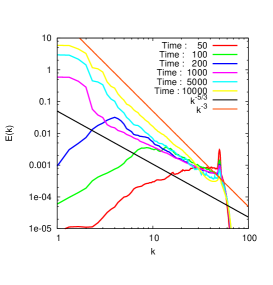
Figure 3: Time evolution of the spectrum showing the transition from a standard $k^{-5/3}$ inverse cascade to a $k^{-3}$ scaling at large scales. Spectra have been locally averaged in time.

So far in this letter we have been discussing the spatio-temporal features of the condensate. Complementarily, and following tradition developed in turbulent studies, one may also analyze velocity spectra. Evolution of the spectra in time is shown in Fig. (3), where one clearly see transition at $t_{*}$ from $k^{-5/3}$ to scaling steeper than $k^{-5/3}$, that is numerically close to $k^{-3}$. Similar statements were made before in Refs. Borue (1994); Tran and Bowman (2004). We claim that this spectrum is spurious and should not be taken as evidence of a cascade in the KLB sense. The coherent part of the flow has almost no fluctuations and, if it is removed, the steeper than $k^{-5/3}$ scaling disappears entirely. By contrast, the $k^{-3}$ enstrophy cascade of KLB involves fluctuating vortices across many scales.

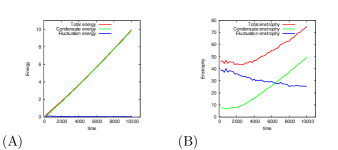
Figure 4: (A) Time evolution of the energy contained in the condensate and background fluctuations (B) enstrophy.

The spectrum of the fluctuations is shown in Fig. 1(F), it is close to $k^{-1}$. There is some evidence that shortly after $\tau_{*}$, the fluctuations retain a $k^{-5/3}$ spectrum as was observed in Borue (1994); Tran and Bowman (2004). However, this regime is transient and does not persist for long after the condensate emerges. Larger resolution will be required to settle this question unambiguously. Fluctuations play a relatively minor role in the overall energy balance with the majority of the energy absorbed into the condensate as shown in Fig. (4)(A). They contain more of the enstrophy as shown in Fig. (4)(B), but they decay in amplitude as the condensate grows so that the flow becomes more and more coherent as time passes. The data suggest that decay of the amplitude of the background fluctuations is logarithmic, or very weakly power law.

We now present an attempt to describe phenomenologically, the universal nature of the asymptotic condensate state. Consider an individual vortex at $t\gg\tau_{*}$. It has a core of radius $\sim l$ and its spatial extent is estimated by the system size, $L$. In discussing the spatial structure of the vortex, for example its mean vorticity profile, $\Omega=\langle\nabla\times{\bm{u}}\rangle$, we will track its dependence on the distance, $r$, from the center of the vortex, $\Omega(r)$. Once the almost circular vortex emerges, it keeps sucking energy from the turbulent background which can be approximately described by an inhomogeneous eddy diffusivity, $D(r)$. Another large scale characteristic affected by the eddy-diffusivity is the fluctuation enstrophy, $H(r)=\langle(\nabla\times{\bm{u}}-\Omega)^{2}\rangle$. The focused regime is adiabatic so that the equations governing the quasi-stationary radially symmetric distribution of $\Omega$ and $H$ on the top of the turbulent background are the eddy-diffusivity equations

$$\partial_{r}rD\partial_{r}\Omega=0,\quad\partial_{r}rD\partial_{r}H=0.$$ (2)

Naturally, $D$ can be expressed in terms of the typical Lyapunov exponent, $\lambda$, $D\sim r^{2}\lambda$. In homogeneneous turbulence $\lambda$ would be self-consistently estimated as $\sim\sqrt{H}$. However present situation is inhomogeneous, with a strong, $\sim\Omega$, shear. Mixing in the presence of strong shear was discussed in Chertkov et al. (2005). It was shown that the dependence of the effective Lyapunov exponent on the mean shear, $\sim\Omega$, and the background enstrophy, $H$, can be estimated as

$$\lambda\sim\left\{\begin{array}[]{cc}H^{1/6}\Omega^{2/3},&\tau_{H}\lambda\ll 1;\\ H^{1/4}\Omega^{1/2},&\tau_{H}\lambda\gg 1.\end{array}\right.$$ (3)

Here $\tau_{H}$ is the correlation time of the background vorticity fluctuations. The actual nonparametric regime we are interested in is $\tau_{H}\lambda\sim 1$. Thus keeping the two asymptotics in Eq. (3) will, in fact, give upper and lower bounds. Returning to Eqs. (2) one notes that the physically meaningful solution for $\Omega$ corresponds to a flux state zero mode of the eddy-diffusivity equation, describing accumulation of the mean vorticity (and the mean energy) inside the vortex, $Dr\partial_{r}\Omega=\mbox{const (wrt }r)$. On the contrary, the physically meaningful solution of the eddy-diffusivity equation for $H$ is the one corresponding to a zero spatial flux, $H=\mbox{const (wrt }r)$. Note, that this spatially homogeneous distribution of $H$ is in agreement with the results of simulations. Combining all these estimations with the global energy conservation one arrives at the following bounds

$$\Omega\sim\frac{\sqrt{\epsilon t}}{r}\left\{\begin{array}[]{cc}(L/r)^{1/5},&\tau_{H}\lambda\ll 1;\\ (L/r)^{1/3},&\tau_{H}\lambda\gg 1.\end{array}\right.$$ (4)

These estimates for the mean vorticity profile are fully consistent, in describing both the overall temporal dynamics and the exponent of the mean vorticity profile, with the aforementioned numerical simulations, shown in Fig. 2: $1/5<\xi\approx 0.25<1/3$. The corresponding estimate for the spatially homogeneous enstrophy, also expressing direct enstrophy balance at the pumping scale, is $H\sim\varepsilon/(l^{2}\lambda)$. This formula, combined with Eq.(3) for the Lyapunov exponent, predicts a slow algebraic decay of the background enstrophy in time. This is again consistent with simulations.

Finally, the spatial homogeneity of $H$ suggests that majority of the injected enstrophy cascades to smaller scales, $r\ll l$. However, a subdominant portion will also penetrate to the larger scales, e.g. resulting in the $k^{-1}$ spectrum observed in the simulations, see Fig. 3. An explanation of the $k^{-1}$ spectrum observed at the scales larger than $l$ after subtraction of the coherent component of the flow is as follows. In a range of scales smaller than $L$ vorticity fluctuations are advected passively. Passive scalar theory, developed in Balkovsky et al. (1999), predicts an $\sim 1/r^{2}$ decay for the pair correlation of a scalar at the scales larger than injection scale in two dimensions and for non-zero value of the Corrsin invariant, which is the integral of the pair correlation function of the pumping. However, vorticity is a curl of velocity injection and thus the vorticity is injected at $l$ with zero value of the Corrsin invariant. This leads to the localized, $\sim\delta({\bm{r}})$, expression for the pair correlation function of vorticity, which in turns translates into the observed $k^{-1}$ spectrum. Notice that similar explanation for this scaling, referred to as passive inverse energy cascade, was reported in Nazarenko and Laval (2000).

To conclude, we performed numerical simulations of energy condensation in forced 2D turbulence. We split the flow into coherent and fluctuating parts, observed the power-like shape of the coherent vortices and self-similar growth in time of the coherent flow. The coherent structure is responsible for the spurious $k^{-3}$ energy spectrum observed in previous numerical experiments. The fluctuations have an energy spectrum of $k^{-1}$ and they diminish in importance as the condensate grows. We also presented phenomenological description of the simulations.

We wish to thank A. Celani, E. Lunasin and L. Smith for advice on numerics and R. Ecke, G. Eyink, G. Falkovich and M. Shats for helpful discussions. This work was carried out under the auspices of the National Nuclear Security Administration of the U.S. Department of Energy at Los Alamos National Laboratory under Contract No. DE-AC52-06NA25396.

References

- Frisch (1995) U. Frisch, Turbulence: The Legacy of A. N. Kolmogorov (Cambridge University Press, Cambridge, 1995).
- Kellay and Goldburg (2002) H. Kellay and W. I. Goldburg, Rep. Prog. Phys. 65, 845 (2002).
- Kraichnan (1967) R. H. Kraichnan, Phys. Fluids 10, 1417 (1967).
- Leith (1968) C. E. Leith, Phys. Fluids 11, 671 (1968).
- Batchelor (1969) G. K. Batchelor, Phys. Fluids 12, 233 (1969).
- Chen et al. (2006) S. Chen, R. Ecke, G. Eyink, M. Rivera, X. Wang, and Z. Xiao, Phys. Rev. Lett. 96, 084502 (2006).
- Smith and Yakhot (1993) L. M. Smith and V. Yakhot, Phys. Rev. Lett. 71, 352 (1993).
- Smith and Yakhot (1994) L. M. Smith and V. Yakhot, J. Fluid. Mech. 274, 115 (1994).
- Paret and Tabeling (1998) J. Paret and P. Tabeling, Phys. Fluids 10, 3126 (1998).
- Jin and Dubin (2000) D. Z. Jin and D. H. E. Dubin, Phys. Rev. Lett. 84, 1443 (2000).
- Shats et al. (2005) M. G. Shats, H. Xia, and H. Punzmann, Phys. Rev. E 71, 046409 (2005).
- Boffetta et al. (2000) G. Boffetta, A. Celani, and M. Vergassola, Phys. Rev. E 61, R29 (2000).
- Boffetta (2006) G. Boffetta, ArXiv e-prints (2006), eprint nlin.CD/0612035.
- Bruneau and Kellay (2005) C. H. Bruneau and H. Kellay, Phys. Rev. E 71, 046305 (2005).
- Lesieur (1997) M. Lesieur, Turbulence in Fluids (Kluwer, Boston, 1997).
- Charney (1971) J. Charney, J. Atm. Sci. 28, 1087 (1971).
- Nastrom and Gage (1985) G. Nastrom and K. Gage, J. Atm. Sci. 49, 950 (1985).
- Molenaar et al. (2004) D. Molenaar, H. J. H. Clercx, and G. J. F. van Heijst, Physica D 196, 329 (2004).
- Danilov and Gurarie (2001) S. Danilov and D. Gurarie, Phys. Rev. E 63, 061208 (2001).
- Farge and Rabreau (1988) M. Farge and G. Rabreau, C.R. Acad. Sci. Paris Sér IIb 307, 1479 (1988).
- Farge et al. (1999) M. Farge, K. Schneider, and K. Kevlahan, Phys. Fluids 11, 2187 (1999).
- Borue (1994) V. Borue, Phys. Rev. Lett. 72, 1475 (1994).
- Tran and Bowman (2004) C. V. Tran and J. C. Bowman, Phys. Rev. E 69, 036303. (2004).
- Chertkov et al. (2005) M. Chertkov, I. Kolokolov, V. Lebedev, and K. Turitsyn, J. Fluid Mech. 531, 251–260 (2005).
- Balkovsky et al. (1999) G. Balkovsky, E. and. Falkovich, V. Lebedev, and M. Lysiansky, Phys. Fluids 11, 2269 (1999).
- Nazarenko and Laval (2000) S. Nazarenko and J.-P. Laval, J. Fluid Mech. 408, 301 (2000).