Abstract

Boolean Delay Equations (BDEs) are semi-discrete dynamical models with Boolean-valued variables that evolve in continuous time. Systems of BDEs can be classified into conservative or dissipative, in a manner that parallels the classification of ordinary or partial differential equations. Solutions to certain conservative BDEs exhibit growth of complexity in time. They represent therewith metaphors for biological evolution or human history. Dissipative BDEs are structurally stable and exhibit multiple equilibria and limit cycles, as well as more complex, fractal solution sets, such as Devil’s staircases and “fractal sunbursts.” All known solutions of dissipative BDEs have stationary variance. BDE systems of this type, both free and forced, have been used as highly idealized models of climate change on interannual, interdecadal and paleoclimatic time scales. BDEs are also being used as flexible, highly efficient models of colliding cascades of loading and failure in earthquake modeling and prediction, as well as in genetics. In this paper we review the theory of systems of BDEs and illustrate their applications to climatic and solid-earth problems. The former have used small systems of BDEs, while the latter have used large hierarchical networks of BDEs. We moreover introduce BDEs with an infinite number of variables distributed in space (“partial BDEs”) and discuss connections with other types of discrete dynamical systems, including cellular automata and Boolean networks. This research-and-review paper concludes with a set of open questions.

Keywords: Discrete dynamical systems, Earthquakes, El-Niño/Southern-Oscillation, Increasing complexity, Phase diagram, Prediction.

PACS:
02.30.Ks (Delay and functional equations)
05.45.Df (Fractals)
91.30.Dk (Seismicity)
92.10.am (El Niño Southern Oscillation)
92.70.Pq (Earth system modeling).

1 Introduction

BDEs are a modeling framework especially tailored for the mathematical formulation of conceptual models of systems that exhibit threshold behavior, multiple feedbacks and distinct time delays [1, 2, 3, 4]. BDEs are intended as a heuristic first step on the way to understanding problems too complex to model using systems of partial differential equations at the present time. One hopes, of course, to be able to eventually write down and solve the exact equations that govern the most intricate phenomena. Still, in the geosciences as well as in the life and other natural sciences, much of the preliminary discourse is often conceptual.

BDEs offer a formal mathematical language that may help bridge the gap between qualitative and quantitative reasoning. Besides, they are fun to play with and produce beautiful fractals by simple, purely deterministic rules. Furthermore, they also provide an unconventional view on the concepts of non-linearity and complexity.

In a hierarchical modeling framework, simple conceptual models are typically used to present hypotheses and capture isolated mechanisms, while more detailed models try to simulate the phenomena more realistically and test for the presence and effect of the suggested mechanisms by direct confrontation with observations [5]. BDE modeling may be the simplest representation of the relevant physical concepts. At the same time, new results obtained with a BDE model often capture phenomena not yet found by using conventional tools [6, 7, 8]. BDEs suggest possible mechanisms that may be investigated using more complex models once their “blueprint” is detected in a simple conceptual model. As the study of complex systems garners increasing attention and is applied to diverse areas — from microbiology to the evolution of civilizations, passing through economics and physics — related Boolean and other discrete models are being explored more and more [9, 10, 11, 12, 13].

The purpose of this research-and-review paper is threefold: (i) summarize and illustrate key properties and applications of BDEs; (ii) introduce BDEs with an infinite number of variables; and (iii) explore more fully connections between BDEs and other types of discrete dynamical systems (dDS). Therefore, we first describe the general form and main properties of BDEs and place them in the more general context of dDS, including cellular automata and Boolean networks (Sect. 2). Next, we summarize some applications, to climate dynamics (Sect. 3) and to earthquake physics (Sect. 4); these applications illustrate both the beauty and usefulness of BDEs. In Sect. 5 we introduce BDEs with an infinite number of variables, distributed on a spatial lattice (“partial BDEs”) and point to several ways of potentially enriching our knowledge of BDEs and extending their areas of application. Further discussion and open questions conclude the paper (Sect. 6).

2 Boolean Delay Equations (BDEs)

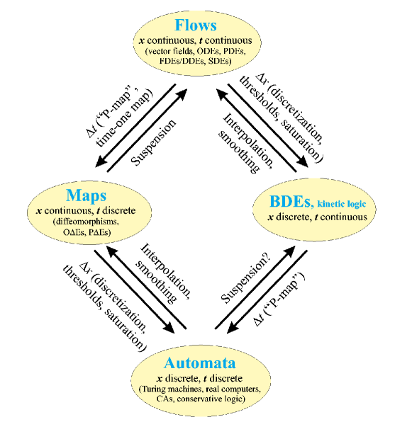
Figure 1: The place of BDEs within dynamical system theory. Note the links: The discretization of $t$ can be achieved by the Poincaré map (P-map) or a time-one map, leading from Flows to Maps. The opposite connection is achieved by suspension. To go from Maps to Automata we use the discretization of $x$. Interpolation and smoothing can lead in the opposite direction. Similar connections lead from BDEs to Automata and to Flows, respectively. Modified after Mullhaupt [2].

BDEs may be classified as semi-discrete dynamical systems, where the variables are discrete — typically Boolean, i.e. taking the values $0$ (“off”) or $1$ (“on”) only — while time is allowed to be continuous. As such they occupy the previously “missing corner” in the rhomboid of Fig. 1, where dynamical systems are classified according to whether their time ($t$) and state variables ($x$) are continuous or discrete.

Systems in which both variables and time are continuous are called flows [14, 15] (upper corner in the rhomboid of Fig. 1). Vector fields, ordinary and partial differential equations (ODEs and PDEs), functional and delay-differential equations (FDEs and DDEs) and stochastic differential equations (SDEs) belong to this category. Systems with continuous variables and discrete time (middle left corner) are known as maps [16, 17] and include diffeomorphisms, as well as ordinary and partial difference equations (O$\triangle$Es and P$\triangle$Es).

In automata (lower corner) both the time and the variables are discrete; cellular automata (CAs) and all Turing machines (including real-world computers) are part of this group [10, 11, 18], and so is the synchronous version of Boolean random networks [12, 19]. BDEs and their predecessors, kinetic [20] and conservative logic, complete the rhomboid in the figure and occupy the remaining middle right corner.

The connections between flows and maps are fairly well understood, as they both fall in the broader category of differentiable dynamical systems (DDS [14, 15, 16]). Poincaré maps (“P-maps” in Fig. 1), which are obtained from flows by intersection with a plane (or, more generally, with a codimension-1 hyperplane) are standard tools in the study of DDS, since they are simpler to investigate, analytically or numerically, than the flows from which they were obtained. Their usefulness arises, to a great extent, from the fact that — under suitable regularity assumptions — the process of suspension allows one to obtain the original flow from its P-map; hence the properties of the flow can be deduced from those of the map, and vice-versa.

In Fig. 1, we have outlined by labeled arrows the processes that can lead from the dynamical systems in one corner of the rhomboid to the systems in each one of the adjacent corners. Neither the processes that connect the two dDS corners, automata and BDEs, nor these that connect either type of dDS with the adjacent-corner DDS — maps and flows, respectively — are as well understood as the (P-map, suspension) pair of antiparallel arrows that connects the two DDS corners. We return to the connection between BDEs and Boolean networks in Sect. 2.6 below. The key difference between kinetic logic and BDEs is summarized in Appendix A.

2.1 General form of a BDE system

Given a system with $n$ continuous real-valued state variables ${{\bf{v}}=(v_{1},v_{2},\dots,v_{n})}$
$\in{\mathbb{R}}^{n}$ for which natural thresholds $q_{i}\in{\mathbb{R}}$ exist, one can associate with each variable $v_{i}\in{\mathbb{R}}$ a Boolean-valued variable, $x_{i}\in{\mathbb{B}}=\{0,1\}$, i.e., a variable that is either ”on” or ”off,” by letting

$$x_{i}=\left\{\begin{array}[]{cc}0,&v_{i}\leq q_{i}\\ 1,&v_{i}>q_{i}\end{array}\right.,\qquad i=1,\dots,n.$$ (1)

The equations that describe the evolution in time of the Boolean vector ${\bf{x}}=(x_{1},x_{2},\dots,x_{n})\in{\mathbb{B}}^{n}$ due to the time-delayed interactions between the Boolean variables $x_{i}\in{\mathbb{B}}$ are of the form:

$$\left\{\begin{array}[]{c}x_{1}(t)=f_{1}\left[\vphantom{\sum^{1}}t,x_{1}(t-\theta_{11}),x_{2}(t-\theta_{12}),\dots,x_{n}(t-\theta_{1n})\right],\\ x_{2}(t)=f_{2}\left[\vphantom{\sum^{1}}t,x_{1}(t-\theta_{21}),x_{2}(t-\theta_{22}),\dots,x_{n}(t-\theta_{2n})\right],\\ \quad\vdots\\ x_{n}(t)=f_{n}\left[\vphantom{\sum^{1}}t,x_{1}(t-\theta_{n1}),x_{2}(t-\theta_{n2}),\dots,x_{n}(t-\theta_{nn})\right].\end{array}\right.$$ (2)

Here each Boolean variable $x_{i}$ depends on time $t$ and on the state of the other variables $x_{j}$ in the past. The functions $f_{i}:{\mathbb{B}}^{n}\rightarrow{\mathbb{B}}$, $1\leq i\leq n$, are defined via Boolean equations that involve logical operators (see Table 1). Each delay value $\theta_{ij}\in{\mathbb{R}}$, $1\leq i,j\leq n$, is the length of time it takes for a change in variable $x_{j}$ to affect the variable $x_{i}$. One always can normalize delays $\theta_{ij}$ to be within the interval $(0,\,1]$ so the largest one has actually unit value; this normalization will always be assumed from now on.

Following Dee and Ghil [1], Mullhaupt [2], and Ghil and Mullhaupt, [3] we consider in this section only deterministic, autonomous systems with no explicit time dependence. Periodic forcing is introduced in Sect. 3, and random forcing in Sect. 4. In Sects. 2–4 we consider only the case of $n$ finite (“ordinary BDEs”), but in Sect. 5 we allow $n$ to be infinite, with the variables distributed on a regular lattice (“partial BDEs”).

2.2 Essential theoretical results on BDEs

We summarize here the most important theoretical results from BDE theory; their original and complete form appears in [1, 2, 3].

We start by choosing a proper topology for the study of BDEs. Denoting by $\mathbb{B}^{n}[0,\,1]$ the space of Boolean-valued vector functions with a finite number of jumps in the interval $[0,1]$:

$${\bf{x}}\mid_{[0,1]}\equiv{\bf{x}}(t\,:\,0\leq t\leq 1),$$

and noting that, $\forall\tau,{\bf{x}}\mid_{[\tau,\tau+1]}$ still belongs to $\mathbb{B}^{n}[0,\,1]$ apart from a translation in time, the system (2) can be considered as an endomorphism:

$$\mathcal{F}_{f}\,:\,\mathbb{B}^{n}[0,1]\rightarrow\mathbb{B}^{n}[0,1].$$ (3)

We wish to extend this endomorphism into one that acts on the solutions ${\bf{x}}(t)$ of Eq. (2):

$$\mathcal{F}_{f}\,:\,{\bf{x}}\mid_{[t,\,t+1]}\rightarrow{\bf{x}}\mid_{[t+1,\,t+2]}.$$ (4)

Changing the point of view between (2) and (4) helps us study the dynamical properties of BDEs. The space $\mathbb{B}^{n}[0,\,1]$ equipped with Boolean algebra [21] and the topology induced by the $L_{1}$ metric:

$$d({\bf{x}},{\bf{y}})\equiv\int_{0}^{1}\sum_{i=1}^{n}|x_{i}(t)-y_{i}(t)|\,dt,$$ (5)

is the phase space on which $\mathcal{F}$ acts; we denote it by $X$. In coding theory, this metric is often called the Hamming distance.

In constructing solutions for a given BDE system, there is a certain similarity with the theory of real-valued delay-differential equations (DDEs) (see [22, 23, 24, 25]), as well as with that of ordinary difference equations (O$\Delta$Es) ([26, 27]).

Theorem 2.1 (Existence and uniqueness) Let ${\bf{x}}\mid_{[0,1]}\in\mathbb{B}^{n}[0,1]$ be the initial data of the dDS (4). Then the equivalent system (2) has a unique solution for all $t\geq 1$ and for an arbitrary $n^{2}$-vector of delays $\Theta=(\theta_{ij})\in(0,\,1]^{n^{2}}$.

Sketch of Proof: The theorem can be proved by induction, constructing an algorithm that advances the solution in time and using a lemma that shows the number of jumps (between the values 0 and 1) to be bounded from above in any finite time interval [1]. Thus the iterates $\mathcal{F}^{k},\>k=1,\dots,K$, stay within $\mathbb{B}^{n}[0,1]$ for all finite $K$ and the unique solution of (2) is given simply by piecing together the successive intervals $[0,1],[1,2],\dots,[K,K+1]$, etc.  

Theorem 2.2 (Continuity) The endomorphism $\mathcal{F}:X\to X$ is continuous for given delays. Moreover, the endomorphism $\mathcal{F}:X\times[0,\,1]^{n^{2}}\to X\times[0,\,1]^{n^{2}}$ is continuous, where the space of delays $(0,\,1]^{n^{2}}$ has the usual Euclidean topology.

At this point, we need to make the critical distinction between rational and irrational delays. All BDE systems that possess only rational delays can be reduced in effect to finite cellular automata. Commensurability of the delays creates a partition of the time axis into segments over which state variables remain constant and whose length is an integer multiple of the delays’ least common denominator (lcd). As there is only a finite number of possible assignments of two values to these segments, repetition must occur, and the only asymptotic behavior possible is eventual constancy or periodicity in time. Thus, we obtain the following

Theorem 2.3 (“Pigeon-hole” lemma) All solutions of (2) with rational delays $\Theta\in\mathbb{Q}^{n^{2}}$ are eventually periodic.

Remark. By “eventually” we mean that a finite-length transient may occur before periodicity sets in. An interesting feature of BDEs $vs.$ flows or maps, as we shall see, is precisely that such transients have finite rather than infinite duration, i.e., asymptotic behavior is reached in finite time.

Dee and Ghil [1], though, found that for the simple system of two BDEs:

$$\left\{\begin{array}[]{lcl}x_{1}(t)&=&x_{2}(t-\theta)\\ x_{2}(t)&=&x_{1}(t-\theta)\bigtriangledown x_{2}(t-1),\end{array}\right.$$ (6)

where $\bigtriangledown$ is the exclusive OR (see Table 1), the number of jumps per unit time seemed to keep increasing with time (see Fig. 2) for a rational value $\theta=0.977$. Complex, aperiodic behavior only arises in cellular automata for an infinite number of variables (also called sites). Thus BDEs seem to pose interesting new problems, irreducible to cellular automata. One of these, at least, is the question of which BDEs, if any, do posses solutions of increasing complexity. To answer this question, we need to classify BDEs and to study separately the effects of rational and irrational delays.

2.3 Classification of BDEs

Based on the pigeon-hole lemma, and therefore on the behavior for rational delays, Ghil and Mullhaupt [3] classified BDE systems as follows. All systems with solutions that are immediately periodic, for any initial data, are conservative; all other systems are dissipative and for some initial data will exhibit transient behavior before settling into eventual periodicity or quasi-periodicity. The DDS analogs are conservative (e.g., Hamiltonian) dynamical systems [28, 29] versus forced-dissipative systems (e.g., the well-known Lorenz system [30]). Typical examples of conservative systems occur in celestial mechanics [31, 32], while dissipative systems are often used in modeling geophysical [33, 34] and many other natural phenomena.

The simplest nontrivial examples of a conservative and a dissipative BDE are

$$x(t)=\overline{x}(t-1)$$

and

$$x(t)=x(t-1)\wedge x(t-\theta),\quad 0<\theta<1,$$

respectively. The Boolean operators we use are listed in Table 1. It is common to call a Boolean function $f=(f_{1},\dots,f_{n})$ a connective and its arguments $x_{i}$ channels [21]; we shall also refer to a channel $x_{i}$ simply as channel $i$.

Definition 2.1 A BDE system is conservative for an open set $\Omega\subset(0,\,1]^{n^{2}}$ of delays if for all rational delays in $\Omega$ and all initial data there are no transients; otherwise the system is dissipative.

As is also the case in DDS theory, the conservative character of a BDE is tightly connected with its time reversibility.

Definition 2.2 A BDE system is reversible if its time reversal also defines a system of BDEs.

Theorem 2.4 (Conservative $\Leftrightarrow$ Reversible) Definitions 2.1 and 2.2 are equivalent.

Useful algebraic criteria have been established [2, 3] for linear or partially linear systems of BDEs to be conservative. Consider the following system

$$x_{i}(t)=\sum_{j=1}^{n}c_{ij}\,x_{j}(t-\theta_{ij})\oplus g_{i}[x_{j^{\prime}}(t-\theta_{ij^{\prime}})],\quad 1\leq i\leq n;$$ (7)

here $\oplus$ and the summation symbol stand for addition (mod 2) in $X$; $c_{ij}\in\mathbb{Z}_{2}$, where $\mathbb{Z}_{2}$ is the field $\{0,1\}$ associated with this addition, while the $g_{i}$ depend only on those $x_{j^{\prime}}$ for which $c_{ij^{\prime}}=0$. Note that $x\bigtriangledown y=x\oplus y$, while $x\bigtriangleup y=1\oplus x\oplus y$. We use the two types of symbols, $\bigtriangledown$ and $\oplus$, interchangeably, depending on the context or point of view.

Adding constants $c_{i0}$ to the above equations corresponds to adding particular “inhomogeneous” solutions to the homogeneous linear system. All solutions of the full system can be represented as the sum of solutions to inhomogeneous and homogeneous systems. We review below only the homogeneous case.

We call a system linear if and only if (iff) all $g_{i}=0$. Naturally, the system obtained by putting $g_{i}=0$ in (7) is called the linear part of the BDE system. Note that this concept of linearity (mod 2) is actually very nonlinear over the field of reals $\mathbb{R}$, with usual addition and multiplication: it corresponds, in a sense, to the thresholding involved in Eq. (1).

First we consider the simplest case of systems with distinct rational delays in their linear part. With any such system we associate its characteristic polynomial

$$Q(z)=\det A(z),\quad A_{ij}=\delta_{ij}+c_{ij}z^{p_{ij}},\quad p_{ij}=q\,\theta_{ij},$$ (8)

where $q$ is the lcd of all the delays $\theta_{ij}$ such that $c_{ij}\neq 0$; the degree of $Q$ is denoted by $\partial Q$.

Theorem 2.5 (Conservativity for linear systems with distinct rational delays) A linear system of BDEs is conservative for an open neighborhood $\Omega$ of a fixed vector of distinct rational delays $\Theta$ iff

$$\sum_{i}q\,\sup_{k}\,\theta_{ki}=\partial Q.$$

In the case of rational delays only, we can give a first definition of partial linearity, namely that at least one $g_{i}\neq 0$ and $\partial Q\geq 2$.

Corollary 2.1 (Partially linear systems) The same result holds for a partially linear system of BDEs with distinct rational delays.

2.4 Solutions with increasing complexity

A natural question is whether (eventually) periodic solutions are generic in a BDE realm? We already noticed (see Fig. 2) that the answer to this question could be negative. Let us introduce the jump counting function

$$J(t)=\#\{{\mbox{jumps~{}of~{}}}{\bf{x}}(t){\mbox{~{}within~{}the~{}interval~{}}}[t,\,{t}+1)\},$$

which measures the complexity of a BDE solution ${\bf{x}}(t)$ with a given set of initial data.

Lemma 2.1 (Increasingly complex solutions for linear BDEs) All solutions (except the trivial one $x(t)\equiv 0$) of the linear scalar BDE

$$x(t)=x(t-1)\bigtriangledown x(t-\theta_{2})\bigtriangledown\dots\bigtriangledown x(t-\theta_{\delta})$$ (9)

with rationally independent $0<\theta_{\delta}<\dots<\theta_{2}<\theta_{1}=1$ and $\delta\geq 2$ are aperiodic and such that the lower bound for the corresponding $J(t)$ increases with time.

A simple example of this increasing complexity is given in Fig. 3, for $\delta=2$, $\theta_{2}\equiv\theta=(\sqrt{5}-1)/2$, and a single jump in the initial data. Note that this delay is equal to the “golden ratio,” which is the most irrational number in the sense that its continued fraction expansion has the slowest possible convergence [35].

Remark. As for ODEs, a “higher-order” BDE can easily be written as a set of “first-order” BDEs (2). Therefore the previous lemma also applies to the system (6) of two linear BDEs, showing that the complexity of the solution is really increasing with time at least for irrational $\theta$.

A more general result holds for partially linear systems that include irrational delays. For such systems of the form (7), we introduce a generalized characteristic polynomial (GCP):

$$Q(\lambda)=\det\,A(\lambda),\quad A_{ij}(\lambda)=\delta_{ij}+c_{ij}\lambda^{{\theta}_{ij}}.$$

Clearly, this polynomial reduces to the characteristic polynomial in (8) if all the delays are rational and $\lambda=z^{q}$. The index $\nu$ of the GCP is defined as the number of its terms. We say that a BDE system (7) is partially linear if at least one $g_{i}\neq 0$ and $\nu$ is large enough, $\nu\geq 3$.

Theorem 2.6 (Increasingly complex solutions for partially linear BDEs) A partially linear system of BDEs has aperiodic solutions of increasing complexity, i.e. with increasing $J(t)$, if its linear part contains $\delta\geq 2$ rationally independent delays.

The condition in this theorem is sufficient, but not necessary. A simple counterexample is given by the third-order scalar BDE

$$x(t)=\left[x(t-1)\bigtriangledown x(t-\theta)\right]\wedge\overline{x}(t-\tau),$$ (10)

with $\theta$, $\tau$, and $\theta/\tau$ irrational, and a single jump in the initial data at $t_{0}$: $0<1-\theta<1-\tau<t_{0}<1$. The jump function for this solution grows in time like that of Eq. (9) for $\delta=2$, although the GCP is identically 1, so that its index is $\nu=1$.

On the other hand, there exist nonlinear BDE systems with arbitrarily many incommensurable delays that have only periodic solutions. For example, all solutions of

$$\overline{x}(t)=\prod_{k=1}^{n}x(t-\theta_{k})$$ (11)

are eventually periodic, with period $\pi=\sum\,\theta_{k}$ for $n$ even, and $\pi=2\sum\,\theta_{k}$ for $n$ odd; the length $\lambda$ of transients is bounded by $\lambda\leq\pi$. The multiplication in (11) is in the sense of the field $\mathbb{Z}_{2}$, with $xy\equiv x\wedge y$ (see Table 1).

Dee and Ghil [1] established the upper bound on the jump function, $J(t)\leq K\,t^{l-1}$, where $l$ is, in general, the number of distinct delays and the constant $K$ depends only on the vector of delays $\Theta$. This bound is essential in proving the existence and uniqueness theorem in Sect. 2.2. Moreover, Ghil and Mullhaupt [3] obtained the lower bounds $J(t)=O\left(t^{\log_{2}(\delta+1)}\right)$ for Eq. (9) and $J(t)\geq K^{\prime}t^{\log_{2}\nu}$ for partially linear BDEs with $\delta\geq\nu-1$ rationally independent delays in the linear part. These authors also showed the log-periodic character of the jump function in Fig. 3 (see also Fig. 7 in [3]).

Having summarized these results, we are still left with the question why Fig. 2 here, with $\theta=0.997$ being a rational number, does exhibit increasing complexity? The question is answered by the following “main approximation theorem”.

Theorem 2.7 (Periodic approximation) All solutions to systems of BDEs can be approximated arbitrarily well (with respect to the $L_{1}$-norm of $X$), for a given finite time, by the periodic solutions of a nearby system that has rational delays only.

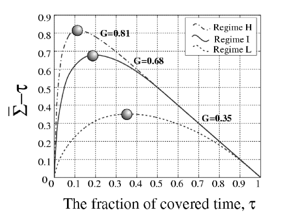
Figure 9: Measure $\mathcal{G}(I)$ of seismic clustering in our BDE model of colliding cascades; see Eq. (26). The three curves correspond to the three synthetic sequences shown in Fig. 7. Reproduced from Zaliapin et al. [7], with kind permission of Springer Science and Business Media.

The apparent paradox is thus solved by taking into account the length of the period obtained for a given conservative BDE and a given rational delay. As the lcd $q$ becomes larger and larger, the solution in Fig. 3 here is well approximated for longer and longer times (see Fig. 9 of [3]); i.e., the jump function can grow for a longer time, before periodicity forces it to decrease and return to a very small number of jumps per unit time.

Since the irrationals are metrically pervasive in $\mathbb{R}^{n}$, i.e., they have measure one, it follows that our chances of observing solutions of conservative BDEs with infinite — or, by the approximation theorem, arbitrarily long — period are excellent. In fact, the solution shown in Fig. 2 here was discovered pretty much by chance, as soon as Dee and Ghil [1] considered a conservative system.

Ghil and Mullhaupt [3] studied, furthermore, the dependence of period length on the connective $f$ and the delay vector $\Theta$, as well as the degree of intermittency of self-similar solutions with growing complexity. In the latter case, we can consider each solution as a transient of infinite length. As we shall see next, such transients preclude structural stability.

2.5 Dissipative BDEs and structural stability

The concept of structural stability for BDEs is patterned after that for DDS. Two systems on a topological space $X$ are said to be topologically equivalent if there exists a homeomorphism $h:X\to X$ that maps solution orbits from one system to those of the other. The system is structurally stable if it is topologically equivalent to all systems in its neighborhood [15, 36].

In discussing structural stability, we are interested in small deformations of a BDE leading to small deformations in its solution. A BDE can be changed by changing either its connective $f$ or its delay vector $\Theta$. Changes in $f$ have to be measured in a discrete topology and cannot, therefore, be small. It suffices thus to consider small perturbations of the delays.

Theorem 2.8 (Structural stability) A BDE system is structurally stable iff all transients and all periods are bounded over some neighborhood $U\subset\mathbb{R}^{n^{2}}$ of its delay vector $\Theta$.

The periodic approximation theorem (Theorem 2.7) implies that, for BDEs like for DDSs, conservative systems are not structurally stable in $X\times[0,1]^{n^{2}}$. Moreover, the conservative “vector fields,” here as there, are in some sense “rare”; for BDEs they are just the three connectives $\overline{x}$, $x\bigtriangledown y$, and $x\bigtriangleup y$, for which the number of 0’s equals the number of 1’s in the “truth table.” Incidentally, the jump set on the delay lattice (see Figs. 1 and 3 of [3]), and hence the growth of $J(t)$, is exactly the same when replacing $f(x,y)=x\bigtriangledown y$ by $f(x,y)=x\bigtriangleup y$ [3].

The structural instability and the rarity of conservative BDEs justifies studying in greater depth dissipative BDEs. Ghil and Mullhaupt [3] concentrated on the scalar $n$th-order BDE

$$x(t)=f[x(t-\theta_{1}),\dots,x(t-\theta_{n})].$$ (12)

The connective $f$ is most conveniently expressed in its normal forms from switching and automata theory, with $xy=x\wedge y$ and $x+y=x\vee y$. With this notation, the disjunctive and conjunctive normal forms represent $f$ as a sum of products and a product of sums, respectively. This formalism helps prove that certain BDEs of the form (12) lead to asymptotic simplification, i.e., after a finite transient, the solution of the full BDE satisfies a simpler BDE. An illustrative example is

$$x(t)=x(t-\theta_{1})\,\overline{x}(t-\theta_{2}),$$ (13)

where either $\theta_{1}$ or $\theta_{2}$ can be the larger of the two. Asymptotically, the solutions of Eq. (13) are given by those of a simpler equation

$$x(t)=x(t-\theta_{1}).$$

Comparison with the asymptotic behavior of forced-dissipative systems in the DDS framework shows two advantages of BDEs. First, the asymptotic behavior sets in after finite (rather than infinite) time. Second, the behavior on the “inertial manifold” or “global attractor” here can be described explicitly by a simpler BDE, while this is rarely the case for a system of ODEs, FDEs, or PDEs.

Finally, one can study asymptotic stability of solutions in the $L_{1}$-metric of $X$. We conclude this theoretical section by recalling that, for $0<\theta<1$ irrational, the solutions of

$$x(t)=x(t-\theta)\,x(t-1)$$

are eventually equal to $x(t)\equiv 0$, except for $x(t)\equiv 1$, which is unstable. Likewise, for

$$x(t)=x(t-\theta)+x(t-1),$$

$x(t)\equiv 1$ is asymptotically stable, while $x(t)\equiv 0$ is not. More generally, one has the following

Theorem 2.9 Given rationally unrelated delays $\Theta=\{\theta_{k}\}$, the BDE

$$x(t)=\prod_{k=1}^{n}x(t-\theta_{k})$$

has $x(t)\equiv 0$ as an asymptotically stable solution, while for the BDE

$$x(t)=\sum_{k=1}^{n}x(t-\theta_{k}),$$

$x(t)\equiv 1$ is asymptotically stable.

To complete the taxonomy of solutions, we also note the presence of quasi-periodic solutions; see discussion of Eq. (6.18) in Ghil and Mullhaupt [3].

Asymptotic behavior. In summary, the following types of asymptotic behavior were observed and analyzed in BDE systems: (a) fixed point — the solution reaches one of a finite number of possible states and remains there; (b) limit cycle — the solution becomes periodic; (c) quasi-periodicity — the solution is a sum of several incommensurable “modes”; and (d) growing complexity — the solution’s number of jumps per unit time increases with time. This number grows like a positive, but fractional power of time $t$ [1, 2], with superimposed log-periodic oscillations [3].

2.6 BDEs, cellular automata (CAs) and Boolean networks

We complete here the discussion of Fig. 1 about the place of BDEs in the broader context of dynamical systems in general. Specifically, we concentrate on the relationships between BDEs and other dDS, to wit cellular automata and Boolean networks.

The formulation of BDEs was originally inspired by advances in theoretical biology, following Jacob and Monod’s discovery [37] of on-off interactions between genes, which had prompted the formulation of “kinetic logic” [20, 38, 39] and Boolean regulatory networks [12, 19, 42]. In the following, we briefly review the latter and discuss their relations with systems of BDEs, whereas kinetic logic is touched upon in Appendix A.

In order to understand the links between BDEs and Boolean regulatory networks it is important to start by recalling some well known definitions and results about cellular automata (CAs), which were introduced by von Neumann already in the late 1940s [18]. Doing so here will also facilitate the discussion of our preliminary results on “partial BDEs” in Sect. 5.

One defines a CA as a set of $N$ Boolean variables $\{x_{i}:\>i=1,\dots,N\}$ on the sites of a regular lattice in $D$ dimensions. The variables are usually updated synchronously according to the same deterministic rule $x_{i}(t)=f[x_{i}(t-1),\dots,x_{N}(t-1)]$; that is the value of each variable $x_{i}$ at epoch $t$ is determined by the values of this and possibly some other variables $\{x_{j}\}$ at the previous epoch $t-1$. In the simplest case of $D=1$ (i.e., of a 1-D lattice) and first-neighbor interactions only, there are $2^{8}$ possible rules $f:\mathbb{B}^{3}\rightarrow\mathbb{B}$, which give 256 different elementary CAs (ECAs) studied in detail by Wolfram [11, 40]. For a given $f$, they evolve according to:

$$x_{i}(t)=f[x_{i-1}(t-1),x_{i}(t-1),x_{i+1}(t-1)],\hskip 21.68121pt1\leq i\leq N,$$ (14)

For a finite size $N$, Eq. (14) is a particular case of a BDE system (2) with connective $f_{i}=f$ for all $i$ and a single delay $\theta_{ij}=1$ for all $i$ and $j$ (see also Sect. 5). One generally speaks of asynchronous CAs when variables at different sites are updated at different $discrete$ times according to some deterministic scheme. Such asynchronous CAs still belong to a restricted class of BDEs with integer delays $\theta_{ij}\in\mathbb{N}$.

When both the space and the time are discrete, a finite-size CA will ultimately display either a fixed-point or periodic behavior. An important advantage of the great simplicity of ECAs is that it allows for systematic studies and helps understand their behavior in the limit of $N\rightarrow\infty$. It can be shown that different updating rules can lead to very different long-time dynamics. Wolfram [40, 41] divided ECAs into four universality classes, according to the typical behavior observed for random initial states and large sizes $N$: For rules in the first class the system evolves towards a fixed point. For rules in the second class the dynamics can attain either a fixed point or a limit cycle, but in this case the period is usually small and it remains small for increasing $N$-values. For rules in the third class, though, the period of the limit cycle usually increases with the size $N$ and it can diverge in the limit $N\rightarrow\infty$, leading to “chaotic” behavior. Finally, CAs in the fourth class are capable of universal computation and are thus equivalent to a Turing machine.

A first generalization of CAs are Boolean networks, in which the Boolean variables $\{x_{i}:\>i=1,2,\dots,N\}$ are attached to the nodes (also called vertices) of a (possibly directed) graph and they evolve synchronously according to deterministic Boolean rules, which may vary from node to node. A further generalization is obtained by considering randomness, in the connections and/or in the choice of updating rules. In particular, the $NK$ model introduced by Kauffman [19, 42], is among the most extensively analyzed random Boolean networks (RBNs). This model considers a system of $N$ Boolean variables such that each value $x_{i}$ depends on $K$ randomly chosen other variables $x_{j}$ through a Boolean function drawn randomly and independently from ${2^{2}}^{K}$ possible variants. The connections among the variables and the updating functions are fixed during a given system’s evolution, and one looks for average properties at long times. Since the variables are updated synchronously, at the same $discrete$ $t$-values, the evolution will ultimately reach a fixed point or a limit cycle for any given configuration of links and rules.

Kauffman [19, 42] proposed such $NK$ RBNs as models of a regulatory genetic network, with different nodes corresponding to different genes. The activity of a gene $x_{i}$ is regulated by the activity of the other $K$ genes to which $x_{i}$ is connected. The different attractors, whether fixed point or limit cycle, are related to different gene expression patterns. In this interpretation, a limit cycle, i.e. a recurrent pattern, corresponds to a cell type and the period is that of the cell cycle.

The $NK$ model was initially studied for a uniform distribution of the updating rules. In this situation, for small $K$ values, one finds on average a small number of fixed points and limit cycles. The lengths of the possible attractors remain finite in the limit of $N\rightarrow\infty$, and therefore the network dynamics appears “ordered.” For large $K$ values, though, the model displays “chaotic” behavior; in this case, the average number of attractors as well as their average length diverge with $N$ and the difference between two almost identical initial states can increase exponentially with time. Furthermore, one observes a transition in parameter space between typical dynamics that is characterized by a large connected cluster of frozen variables and the opposite one with small separated clusters of frozen variables. The critical values of the parameters corresponding to this passage from an “ordered” to a “chaotic” regime can be evaluated by looking at the evolution of the Hamming distance between two trajectories that start from slightly different configurations [43, 44, 45]. In particular, for a uniform distribution of the Boolean updating functions, the $NK$ model is “critical” when $K=2$.

Kauffman [19] suggested that natural organisms could lie on or near the borderline between these two different dynamical regimes, i.e. “at the edge of chaos,” where the system is still sufficiently robust against small perturbations but at the same time close enough to the chaotic regime to feel the effect of selection. Accordingly, a lot of attention has been devoted to the study of such critical networks, which can also be obtained for $K>2$ with appropriate, and possibly more realistic, choices of the updating rule distribution. Similar edge-of-chaos suggestions have been made in other applications of dynamical systems theory, including DDS and celestial mechanics [46].

For large $N$-values, even the problem of determining the fixed points of a generic regular RBN, with $K_{i}=K$ for all $i$, is highly nontrivial. In the context of the modeling of genetic interactions, the solution to this problem is thought to represent different accessible states of the cell, possibly triggered by external inputs [47]. This problem has been recently reformulated [47, 48] in terms of the zero-energy configurations of an appropriate Hamiltonian. In this formulation, statistical mechanics tools from spin-glass physics can be brought to bear on the problem; these tools have also been successfully extended to general optimization issues [49].

Irregular RBNs, in which the number of inputs $K_{i}$ is also a node-dependent random variable, are obviously harder to analyze. There is increasing evidence [50] that many networks arising in very different natural contexts are “scale free,” i.e. their node-dependent connectivity $K_{i}$ is distributed according to a power law $\mathsf{P}(K_{i})\propto{K_{i}}^{-\gamma}$. This seems to be true as well for the distribution of the input connections of some genetic networks. In the irregular case, too, one still observes “critical” dynamical behavior, given a suitable distribution of the updating Boolean functions. Kauffmann and colleagues [51] have recently studied the stability properties of regular and irregular RBNs and their dependence on the distribution of connectivity $K_{i}$ and/or Boolean functions. Inverse problems, in which one tries to determine the Boolean rules leading to a particular type of behavior, have been considered in [52].

The dependence of the average number $\bar{m}$ of attractors and of their period length on the size $N$ in critical RBNs is still a matter of debate. This issue is particularly relevant for genetic-network modeling, since the behavior of $\bar{m}(N)$ is expected to be related [19, 43] to the number of cell types which are present in an organism characterized by a given number $N$ of genes. Recent results [53, 54, 55] show that $\bar{m}(N)$ increases faster than any power of $N$ in regular synchronous RBNs, in which all variables are updated in parallel at the same discrete epochs. These findings suggest that using different updating schemes could lead to more realistic behavior, with a slower increase of $\bar{m}(N)$. Moreover, assuming that all the variables act synchronously, i.e. that they “move in lock-step,” may be too drastic a simplification for correctly modeling a number of natural systems and, in particular, interacting genes [56]. In order to overcome this simplification, asynchronous Boolean networks with different updating procedures have been studied recently [57]. A recent review [56] underlines the links of such generalized RBNs with asynchronous CAs and with “kinetic logic.”

From the point of view of connections with BDEs, the updating scheme introduced by Klemm and Bornholdt [58] is of particular interest; they consider a “critical” regular RBN with $K=2$ and weakly fluctuating delays in the response of each node. The number of stable attractors in this system increases more slowly with system size than for synchronous updating. It seems therefore that RBNs in continuous time may be more realistic and may exhibit new and possibly unexpected types of behavior.

Öktem et al. [59] have recently applied a BDE approach to a Boolean network of genetic interactions with given architecture. In this case continuous time delays are introduced according to the BDE formalism of [1, 2, 3, 4]. As a result, more complicated types of behavior than in synchronously updated Boolean networks have been observed, and the dynamics of the system seems to be characterized by aperiodic attractors.

In both [58] and [59], the authors introduced a minimal time interval below which changes in a given variable are not permitted. Such a cutoff, or “refractory period” [59], may have a physiological basis in genetic applications, but it rules out the presence of solutions with increasing complexity. Therefore, for a finite number of variables, this restriction must result in an ultimately periodic behavior; the asymptotic period, though, could be much larger than the one obtainable with usual Boolean networks, especially when considering conservative connectives and irrational delays. From this point of view, the implementation of continuous time delays in [58, 59] is different than in BDEs [1]-[4] and is similar to the one adopted in “kinetic logic” [20, 38, 39], whose precise connections with our formalism are discussed in Appendix A.

In the applications of BDEs that we review in the next sections, one finds different mechanisms that lead to aperiodic solutions of bounded complexity, without the need of a cutoff; one could thus explore the possibility of similar behavior in genetic-interaction models as well. Summarizing, one can say that kinetic logic and the recently proposed genetic network models [58, 59], as well as others recent generalizations of RBNs with deterministic updating [56], can be viewed either as asynchronous CAs or as particular cases of BDEs with large $N$.

In Sect. 5, we initiate the systematic study of BDE systems in the limit of an infinite number of variables, assumed for the moment to lie on a regular lattice and to interact according to a given, unique, deterministic rule. This study should allow us to better understand the connections of BDEs with (infinite) CAs, on the one hand, and with PDEs on the other. Such a study should also help clarify further the behavior of, possibly random, Boolean networks in continuous time.

We now turn to an illustration of BDE modeling in action, first with a climatic example and then with one from lithospheric dynamics. Both of these applications introduce new and interesting properties of and extensions to BDEs. The climatic BDE model in Sect. 3, while keeping a small number of variables, introduces variables with more than two levels, as well as periodic forcing. Its solutions show that a simple BDE model can mimic rather well the solution set of a much more detailed model, based on nonlinear PDEs, as well as produce new and previously unsuspected results, such as a Devil’s Staircase and a “bizarre” attractor in phase-parameter space.

The seismological BDE model in Sect. 4 introduces a much larger number of variables, organized in a directed graph, as well as random forcing and state-dependent delays. This BDE model also reproduces a regime diagram of seismic sequences resembling observational data, as well as the results of much more detailed models [60, 61] based on a large system of differential equations; furthermore it allows the exploration of seismic prediction methods.

3 A BDE Model for the El Niño/Southern Oscillation

BDEs were first applied to paleoclimatic problems. Ghil et al. [4] used the exploratory power of BDEs to study the coupling of radiation balance of the Earth-atmosphere system, mass balance of continental ice sheets, and overturning of the oceans’ thermohaline circulation during glaciation cycles. On shorter time scales, Darby and Mysak [62] and Wohlleben and Weaver [63] studied the coupling of the sea ice with the atmosphere above and the ocean below in an interdecadal Arctic and North Atlantic climate cycle, respectively. Here we describe an application to tropical climate, on even shorter, seasonal-to-interannual time scales.

The El-Niño/Southern-Oscillation (ENSO) phenomenon is the most prominent signal of seasonal-to-interannual climate variability. It was known for centuries to fishermen along the west coast of South America, who witnessed a seemingly sporadic and abrupt warming of the cold, nutrient-rich waters that support the food chains in those regions; these warmings caused havoc to their fish harvests [64, 65]. The common occurrence of such warming shortly after Christmas inspired them to name it El Niño, after the “Christ child.” Starting in the 1970s, El Niño’s climatic effects were found to be far broader than just its manifestations off the shores of Peru [64, 66, 67]. This realization led to a global awareness of ENSO’s significance, and an impetus to attempt and improve predictions of exceptionally strong El Niño events [68, 69].

3.1 Conceptual ingredients

The following conceptual elements are incorporated into the logical equations of our BDE model for ENSO variability.

(i) The Bjerknes hypothesis: Bjerknes [70], who laid the foundation of modern ENSO research, suggested a positive feedback as a mechanism for the growth of an internal instability that could produce large positive anomalies of sea surface temperatures (SSTs) in the eastern Tropical Pacific. We use here the climatological meaning of the term anomaly, i.e., the difference between an instantaneous (or short-term average) value and the normal (or long-term mean). Using observations from the International Geophysical Year (1957-58), he realized that this mechanism must involve air-sea interaction in the tropics. The “chain reaction” starts with an initial warming of SSTs in the “cold tongue” that occupies the eastern part of the equatorial Pacific. This warming causes a weakening of the thermally direct Walker-cell circulation; this circulation involves air rising over the warmer SSTs near Indonesia and sinking over the colder SSTs near Peru. As the trade winds blowing from the east weaken and give way to westerly wind anomalies, the ensuing local changes in the ocean circulation encourage further SST increase. Thus the feedback loop is closed and further amplification of the instability is triggered.

(ii) Delayed oceanic wave adjustments: Compensating for Bjerknes’s positive feedback is a negative feedback in the system that allows a return to colder conditions in the basin’s eastern part. During the peak of the cold-tongue warming, called the warm or El Niño phase of ENSO, westerly wind anomalies prevail in the central part of the basin. As part of the ocean’s adjustment to this atmospheric forcing, a Kelvin wave is set up in the tropical wave guide and carries a warming signal eastward. This signal deepens the eastern-basin thermocline, which separates the warmer, well-mixed surface waters from the colder waters below, and thus contributes to the positive feedback described above. Concurrently, slower Rossby waves propagate westward, and are reflected at the basin’s western boundary, giving rise therewith to an eastward-propagating Kelvin wave that has a cooling, thermocline-shoaling effect. Over time, the arrival of this signal erodes the warm event, ultimately causing a switch to a cold, La Niña phase.

(iii) Seasonal forcing: A growing body of work [5, 71, 72, 73, 74, 75, 76] points to resonances between the Pacific basin’s intrinsic air-sea oscillator and the annual cycle as a possible cause for the tendency of warm events to peak in boreal winter, as well as for ENSO’s intriguing mix of temporal regularities and irregularities. The mechanisms by which this interaction takes place are numerous and intricate and their relative importance is not yet fully understood [76, 77, 78]. We assume therefore in the present BDE model that the climatological annual cycle provides for a seasonally varying potential of event amplification.

3.2 Model variables and equations

The model [6] operates with five Boolean variables. The discretization of continuous-valued SSTs and surface winds into four discrete levels is justified by the pronounced multimodality of associated signals (see Fig. 1b of [6]).

The state of the ocean is depicted by SST anomalies, expressed via a combination of two Boolean variables, $T_{1}$ and $T_{2}$. The relevant anomalous atmospheric conditions in the Equatorial Pacific basin are described by the variables $U_{1}$ and $U_{2}$. The latter express the state of the trade winds. For both the atmosphere and the ocean, the first variable, $T_{1}$ or $U_{1}$, describes the sign of the anomaly, positive or negative, while the second one, $T_{2}$ or $U_{2}$, describes its amplitude, strong or weak. Thus, each one of the pairs $(T_{1},\,T_{2})$ and $(U_{1},\,U_{2})$ defines a four-level discrete variable that represents highly positive, slightly positive, slightly negative, and highly negative deviations from the climatological mean. The seasonal cycle’s external forcing is represented by a two-level Boolean variable $S$.

The atmospheric variables $U_{i}$ are ”slaved” to the ocean [74, 79]:

$$U_{i}(t)=T_{i}(t-\beta),~{}i=1,2.$$ (15)

The evolution of the sign $T_{1}$ of the SST anomalies is modeled according to the following two sets of delayed interactions:

(i) Extremely anomalous wind stress conditions are assumed to be necessary to generate a significant Rossby-wave signal $R(t)$, which takes on the value $1$ when wind conditions are extreme at the time and $0$ otherwise. By definition strong wind anomalies (either easterly or westerly) prevail when $U_{1}=U_{2}$ and thus $R(t)=U_{1}(t)\bigtriangleup U_{2}(t)$; here $\bigtriangleup$ is the binary Boolean operator that takes on the value $1$ if and only if both operands have the same value (see Sect. 2 and Table 1). A wave signal $R(t)=1$ that is elicited at time $t$ is assumed to re-enter the model system after a delay $\tau$, associated with the wave’s travel time across the basin. Upon arrival of the signal in the eastern equatorial Pacific at time $t+\tau$, the wave signal affects the thermocline-depth anomaly there and thus reverses the sign of SST anomalies represented by $T_{1}$.

(ii) In the second set of circumstances, when $R(t)=0$, and thus no significant wave signal is present, we assume that $T_{1}(t+\tau)$ responds directly to local atmospheric conditions, after a delay $\beta$, according to Bjerknes hypothesis; the delays associated with local coupled processes are taken all equal.

The two mechanisms (i) and (ii) are combined to yield:

$$T_{1}(t)=\left\{\left[R\wedge\overline{U_{1}}\right](t-\tau)\right\}\lor\left\{\overline{R}(t-\tau)\wedge U_{2}(t-\beta)\right\};$$ (16)

here the symbols $\lor$ and $\wedge$ represent the binary logical operators OR and AND, respectively (see Table 1).

The seasonal-cycle forcing $S$ is given by $S(t)=S(t-1)$; the time $t$ is thus measured in units of 1 year. The forcing $S$ affects the SST anomalies’ amplitude $T_{2}$ through an enhancement of events when favorable seasonal conditions prevail:

$$T_{2}(t)=\left\{\left[S\triangle T_{1}\right](t-\beta)\right\}\lor\left\{\left[\overline{(S\triangle T_{1})}\land T_{2}\right](t-\beta)\right\}.$$ (17)

The model’s principal parameters are the two delays $\beta$ and $\tau$ associated with local adjustment processes and with basin-wide processes, respectively. The changes in wind conditions are assumed to lag the SST variables by a short delay $\beta$, of the order of days to weeks. For the length of the delay $\tau$ we adopt Jin’s [80] view of the delayed-oscillator mechanism and let it represent the time that elapses while combined processes of oceanic adjustment occur: it may vary from about one month in the fast-wave limit [81, 82, 83] to about two years.

3.3 Model solutions

Studying the ENSO phenomenon, we are primarily interested in the dynamics of the SST states, represented by the two-variable Boolean vector $(T_{1},\,T_{2})$. To be more specific, we deal with a four-level scalar variable

$$ENSO=\left\{\begin{array}[]{rcl}-2,&{\rm~{}extreme~{}La~{}Ni\tilde{n}a},&T_{1}=0,\,T_{2}=0,\\ -1,&{\rm~{}mild~{}La~{}Ni\tilde{n}a},&T_{1}=0,\,T_{2}=1,\\ 1,&{\rm~{}mild~{}El~{}Ni\tilde{n}o},&T_{1}=1,\,T_{2}=0,\\ 2,&{\rm~{}extreme~{}El~{}Ni\tilde{n}o},&T_{1}=1,\,T_{2}=1.\\ \end{array}\right.$$ (18)

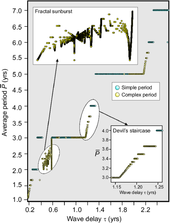
Figure 4: Devil’s staircase and fractal sunburst for a BDE model of the El-Niño/Southern-Oscillation (ENSO) phenomenon. Plotted in the bifurcation diagram is the average cycle length $\bar{P}$ vs. the wave delay $\tau$ for a fixed local delay $\beta=0.17$. Blue dots indicate purely periodic solutions; orange dots are for complex periodic solutions; small black dots denote aperiodic solutions. The two insets show a blow-up of the overall, approximate behavior between periodicities of two and three years (“fractal sunburst”) and of three and four years (“Devil’s staircase”). Modified after Saunders and Ghil [6].

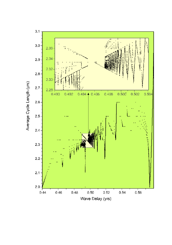
Figure 5: Fractal sunburst: a BDE solution pattern in phase-parameter space, for a dissipative BDE system with periodic forcing. The plot is a blow-up of the transition zone from average periodicity two to three years in Fig. 4; here $\tau=0.44$–$0.58,\beta=0.17$. The inset is a zoom on $0.490\leq\tau\leq 0.504$. A complex mini-staircase structure reveals self-similar features, with a focal point at $\tau\approx 0.5$. Modified after Saunders and Ghil [6].

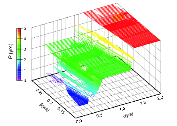
Figure 6: The Devil’s bleachers in our BDE model of ENSO. The three-dimensional regime diagram shows the average cycle length $\bar{P}$, portrayed in both height and color, vs. the two delays $\beta$ and $\tau$. Oscillations are produced even for very small values of $\beta$, as long as $\beta\leq\tau$. Variations in $\tau$ determine the oscillation’s period, while changing $\beta$ establishes the bottom step of the staircase, shifts the location of the steps, and determines their width. After Saunders and Ghil [6].

In all our simulations, this variable takes on the values $\{-2,\,-1,\,1,\,2\}$, precisely in this order, thus simulating real ENSO cycles. The cycles follow the same sequence of states, although the residence time within each state changes as $\tau$ changes at fixed $\beta$. The period $P$ of a simple oscillatory solution is defined as the time between the onset of two consecutive extreme warm events, $ENSO=2$. We use the cycle period definition to classify different model solutions (see Figs. 4–6).

(i) Periodic solutions with a single cycle (simple period). Each succession of events, or internal cycle, is completely phase-locked here to the seasonal cycle, i.e., the warm events always peak at the same time of year. For each fixed $\beta$, as $\tau$ is increased, intervals where the solution has a simple period equal to $2,3,4,5,6$ and $7$ years arise consecutively.

(ii) Periodic solutions with several cycles (complex period). We describe such sequences, in which several distinct cycles make up the full period, by the parameter $\bar{P}=P/n$; here $P$ is the length of the sequence and $n$ is the number of cycles in the sequence. Notably, as we transition from a period of three years to a period of four years (see second inset of Fig. 4), $\bar{P}$ becomes a nondecreasing step function of $\tau$ that takes only rational values, arranged on a Devil’s Staircase.

3.4 The quasi-periodic (QP) route to chaos in the BDE model

The frequency-locking behavior observed for our BDE solutions above is a signature of the universal QP route to chaos. Its mathematical prototype is the Arnol’d circle map [14], given by the equation

$$\theta_{n+1}=\theta_{n}+\Omega+2{\pi}K\sin(2\pi\theta_{n})~{}({\rm mod~{}}1).$$ (19)

Equation (19) describes the motion of a point, denoted by the angle $\theta$ of its location on a unit circle, which undergoes fixed shifts by an angle $\Omega$ along the circle’s circumference. The point is also subject to nonlinear sinusoidal “corrections,” with the size of the nonlinearity controlled by a parameter $K$.

The solutions of (19) are characterized by their winding number

$$\omega=\omega(\Omega,K)=\lim_{n\rightarrow\infty}\left[(\theta_{n}-\theta_{0})/n\right],$$

which can be described roughly as the average shift of the point per iteration. When the nonlinearity’s influence is small, this average shift — and hence the average period — is determined largely by $\Omega$; it may be rational or irrational, with the latter being more probable due to the irrationals’ pervasiveness. As the nonlinearity $K$ is increased, “Arnol’d tongues” — where the winding number $\omega$ locks to a constant rational over whole intervals — form and widen. At a critical parameter value, only rational winding numbers are left and a complete Devil’s Staircase crystallizes. Beyond this value, chaos reigns as the system jumps irregularly between resonances [84, 85].

The average cycle length $\bar{P}$ defined for our ENSO system of BDEs is clearly analogous to the circle map’s winding number, in both its definition and behavior. Note that the QP route to chaos depends in an essential way on two parameters: $\Omega$ and $K$ for the circle map and $\beta$ and $\tau$ in our BDE model.

3.5 The “fractal sunburst”: A “bizarre” attractor

As the system undergoes the transition from an averaged period of two to three years a much more complex, and heretofore unsuspected, “fractal-sunburst” structure emerges (Fig. 5, and first inset in Fig. 4). As the wave delay $\tau$ is increased, mini-ladders build up, collapse or descend only to start climbing up again. In the vicinity of a critical value ($\tau\cong 0.5$ years) that constitutes the pattern’s focal point, these mini-ladders rapidly condense and the structure becomes self-similar, as each zoom reveals the pattern being repeated on a smaller scale. We call this a “bizarre” attractor because it is more than “strange”: strange attractors occur in a system’s phase space, for fixed parameter values, while this fractal sunburst appears in our model’s phase–parameter space, like the Devil’s Staircase. The structure in Fig. 4 is attracting, though, only in phase space, for fixed parameter values; it is, therefore, a generalized attractor, and not just a bizarre one.

The influence of the local-process delay $\beta$, along with that of the wave-dynamics delay $\tau$, is shown in the three-dimensional “Devil’s bleachers” (or “Devil’s terrace,” according to Jin et al. [74]) of Fig. 6. Note that the Jin et al. [73, 74] model is an intermediate model, in the terminology of modeling hierarchies [5], i.e. intermediate between the simplest “toy models” (BDEs or ODEs) and highly detailed models based on discretized systems of PDEs in three space dimensions, such as the general circulation models (GCMs) used in climate simulation. Specifically, the intermediate model of Jin and colleagues is based on a system of nonlinear PDEs in one space dimension (longitude along the equator). The Devil’s bleachers in our BDE model resemble fairly well those in the intermediate ENSO model of Jin et al. [74]. The latter, though, did not exhibit a fractal sunburst, which appears, on the whole, to be an entirely new addition to the catalog of fractals [86, 87, 88].

It would be interesting to find out whether such a bizarre attractor occurs in other types of dynamical systems. Its specific significance in the ENSO problem might be associated with the fact that a broad peak with a period between two and three years appears in many spectral analyses of SSTs and surface winds from the Tropical Pacific [89, 90]. Various characteristics of the Devil’s Staircase have been well documented in both observations [90, 91, 92] and GCM simulations [5, 73] of ENSO. It remains to see whether this will be the case for the fractal sunburst as well.

4 A BDE Model for Seismicity

Lattice models of systems of interacting elements are widely applied for modeling seismicity, starting from the pioneering works of Burridge and Knopoff [93], Allègre et al. [94], and Bak et al. [95]. The state of the art is summarized in [96, 97, 98, 99, 100]. Recently, colliding-cascade models [7, 8, 60, 61] have been able to reproduce a wide set of observed characteristics of earthquake dynamics [101, 102, 103]: (i) the seismic cycle; (ii) intermittency in the seismic regime; (iii) the size distribution of earthquakes, known as the Gutenberg-Richter relation; (iv) clustering of earthquakes in space and time; (v) long-range correlations in earthquake occurrence; and (vi) a variety of seismicity patterns premonitory to a strong earthquake.

Introducing the BDE concept into the modeling of colliding cascades, we replace the elementary interactions of elements in the system by their integral effect, represented by the delayed switching between the distinct states of each element: unloaded or loaded, and intact or failed. In this way, we bypass the necessity of reconstructing the global behavior of the system from the numerous complex and diverse interactions that researchers are only mastering by and by and never completely. Zaliapin et al. [7, 8] have shown that this modeling framework does simplify the detailed study of the system’s dynamics, while still capturing its essential features. Moreover, the BDE results provide additional insight into the system’s range of possible behavior, as well as into its predictability.

4.1 Conceptual ingredients

Colliding-cascade models [7, 8, 60, 61] synthesize three processes that play an important role in lithosphere dynamics, as well as in many other complex systems: (i) the system has a hierarchical structure; (ii) the system is continuously loaded (or driven) by external sources; and (iii) the elements of the system fail (break down) under the load, causing redistribution of the load and strength throughout the system. Eventually the failed elements heal, thereby ensuring the continuous operation of the system.

The load is applied at the top of the hierarchy and transferred downwards, thus forming a direct cascade of loading. Failures are initiated at the lowest level of the hierarchy, and gradually propagate upwards, thereby forming an inverse cascade of failures, which is followed by healing. The interaction of direct and inverse cascades establishes the dynamics of the system: loading triggers the failures, and failures redistribute and release the load. In its applications to seismicity, the model’s hierarchical structure represents a fault network, loading imitates the effect of tectonic forces, and failures imitate earthquakes.

4.2 Model structure and parameters

(i) The model acts on a directed graph whose nodes, except the top one and the bottom ones, have connectivity six. Each node, except the bottom ones, is a parent to three children, that are siblings to each other. This graph is obtained from a directed ternary tree, which has its root in the top element, by connecting siblings, i.e., groups of three nodes that have the same parent.

(ii) Each element possesses a certain degree of weakness or fatigue. An element fails when its weakness exceeds a certain threshold.

(iii) The model runs in discrete time $t=0,1,\dots$. At each epoch a given element may be either intact or failed (broken), and either loaded or unloaded. The state of an element $e$ at a epoch $t$ is defined by two Boolean functions: $s_{e}(t)=0$, if an element is intact, and $s_{e}(t)=1$, if an element is failed; $l_{e}(t)=0$, if an element is unloaded, and $l_{e}(t)=1$, if an element is loaded.

(iv) An element of the system may switch from one state $(s,l)\in\{0,1\}^{2}$ to another under an impact from its nearest neighbors and external sources. The dynamics of the system is controlled by the time delays between the given impact and switching to another state.

(v) At the start, $t=0$, all elements are in the state $(0,0)$, intact and unloaded. Most of the changes in the state of an element occur in the following cycle:

$$(0,0)\rightarrow(0,1)\rightarrow(1,1)\rightarrow(1,0)\rightarrow(0,0)\dots$$

Other sequences, however, are also possible, except that a failed and loaded element may switch only to a failed and unloaded state, $(1,1)\rightarrow(1,0)$. The latter transition mimics fast stress drop after a failure.

(vi) All the interactions take finite, nonzero time. We model this by introducing four basic time delays: $\Delta_{L}$, between being impacted by the load and switching to the loaded state, $(\cdot,0)\rightarrow(\cdot,1)$; $\Delta_{F}$, between the increase in weakness and switching to the failed state, $(0,\cdot)\rightarrow(1,\cdot)$; $\Delta_{D}$, between failure and switching to the unloaded state, $(\cdot,1)\rightarrow(\cdot,0)$; and $\Delta_{H}$, between the moment when healing conditions are established and switching to the intact (healed) state, $(1,\cdot)\rightarrow(0,\cdot)$.

The duration of each particular delay, from one switch of an element’s state to the next, is determined from these basic delays, depending on the state of the element as well as of its nearest neighbors during the preceding time interval (see [7] for details). This represents yet another generalization of the set of deterministic, autonomous equations (2) with fixed delays $\theta_{ij}$: here the effective delays are both variable and state-dependent.

(vii) Failures are initiated randomly within the elements at the lowest level.

The two primary delays in this system are the loading time $\Delta_{L}$ necessary for an unloaded element to become loaded under the impact of its parent, and the healing time $\Delta_{H}$ necessary for a broken element to recover.

Conservation law. The model is forced and dissipative, if we associate the loading with an energy influx. The energy dissipates only at the lowest level, where it is transferred downwards, out of the model. In any part of the model not including the lowest level, energy conservation holds, but only after averaging over sufficiently large time intervals. On small intervals it may not hold, due to the discrete time delays involved in energy transfer.

Model solutions. The output of the model is a catalog ${\mathcal{C}}$ of earthquakes — i.e., of failures of its elements — similar to the simplest routine catalogs of observed earthquakes:

$${\mathcal{C}}=(t_{k},~{}m_{k},~{}h_{k}),~{}k=1,2,\dots;~{}t_{k}\leq t_{k+1}.$$ (20)

In real-life catalogs, $t_{k}$ is the starting time of the rupture; $m_{k}$ is the magnitude, a logarithmic measure of energy released by the earthquake; and $h_{k}$ is the vector that comprises the coordinates of the hypocenter. The latter is a point approximation of the area where the rupture started. In our BDE model, earthquakes correspond to failed elements, $m_{k}$ is the level at which the failed element is situated within the directed graph, while the position of this element within its level is a counterpart of $h_{k}$.

4.3 Seismic regimes

A long-term pattern of seismicity within a given region is usually called a seismic regime. It is characterized by the frequency and irregularity of the strong earthquakes’ occurrence, more specifically by (i) the Gutenberg-Richter relation, i.e. the time-and-space averaged magnitude–frequency distribution; (ii) the variability of this relation with time; and (iii) the maximal possible magnitude. The notion of seismic regime here is a much more complete description of seismic activity than the “level of seismicity,” often used to discriminate among regions with high, medium, low and negligible seismicity; the latter are called aseismic regions.

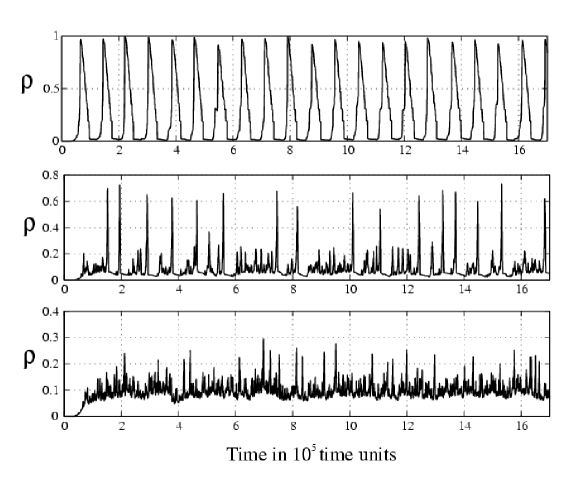
Figure 8: Three seismic regimes: internal dynamics of the BDE model. The panels show the density $\rho(n)$ of broken elements in the system, as defined by Eq. (21); they correspond to the synthetic sequences shown in Fig. 7. Top panel – Regime H; middle panel – Regime I; and bottom panel – regime L. Reproduced from Zaliapin et al. [7], with kind permission of Springer Science and Business Media.

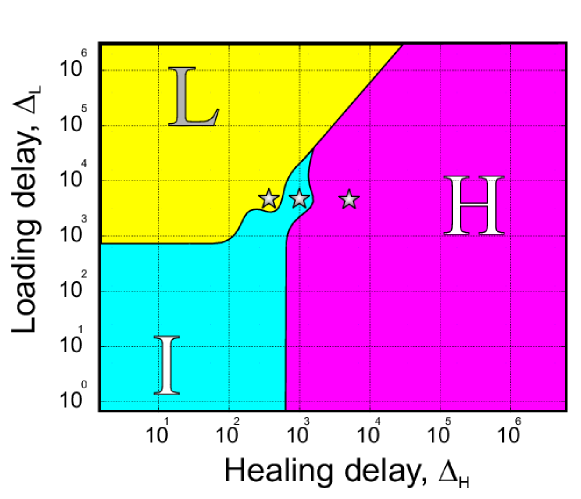
Figure 10: Regime diagram in the $(\Delta_{L},\Delta_{H})$ plane of the loading and healing delays. Stars correspond to the sequences shown in Fig. 7. Reproduced from Zaliapin et al. [7], with kind permission of Springer Science and Business Media.

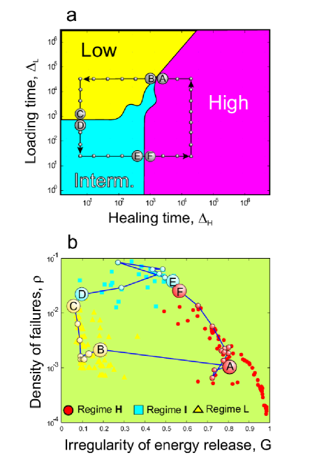
Figure 11: Bifurcation diagram for the BDE seismic model: (a) rectangular path in the delay plane $(\Delta_{L},\,\Delta_{H})$; and (b) the measures $\mathcal{G}$ and $\rho$, calculated along the rectangular path shown in panel (a). The transition between points (A) and (B), i.e. between regimes H and L, is very sharp with respect to the change in irregularity $\mathcal{G}$ of energy release, while almost negligible with respect to the change in failure density $\rho$. The colored circles, triangles, and squares in panel (b) correspond to synthetic catalogs from regimes H, I, and L, respectively; these catalogs are produced for the points indicated along the rectangular path in panel (a), as well as for many scatter points that lie on a uniform grid covering the entire regime diagram, with the same resolution in $\delta_{H}$ and $\delta_{L}$ as those along the path.

The seismic regime is to a large extent determined by the neotectonics of a region; this involves, roughly speaking, two factors: (i) the rate of crustal deformations; and (ii) the crustal consolidation, determining what part of deformations is realized through the earthquakes. However, as is typical for complex processes, the long-term patterns of seismicity may switch from one to another in the same region, as well as migrate from one area to another on a regional or global scale [104, 105]. Our BDE model produces synthetic sequences that can be divided into three seismic regimes, illustrated in Figs. 7–11.

Regime H: High and nearly periodic seismicity (top panel of Figs. 7 and 8). The fractures within each cycle reach the top level, $m=L$, where our underlying ternary graph has depth $L=6$. The sequence is approximately periodic, in the statistical sense of cyclo-stationarity [106].

Regime I: Intermittent seismicity (middle panel of Figs. 7 and 8). The seismicity reaches the top level for some but not all cycles, and cycle length is very irregular.

Regime L: Medium or low seismicity (lower panel of Figs. 7 and 8). No cycle reaches the top level and seismic activity is much more constant at a low or medium level, without the long quiescent intervals present in Regimes H and I.

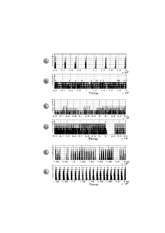
Figure 12: Synthetic sequences corresponding to the key points along the rectangular path in parameter space of Fig. 11a. The panels illustrate the transitions between the regimes H and L — panels (A) and (B); L and I — (C) and (D); and I and H — (E) and (F). The transition from (A) to (B) is very pronounced, while the other two transitions are smoother. Reproduced from Zaliapin et al. [7], with kind permission of Springer Science and Business Media.

The location of these three regimes in the plane of the two key parameters $(\Delta_{L},\Delta_{H})$ is shown in Fig. 10. Figures 7–12 were computed for a tree depth of $L=6$, i.e. 1093 nodes. Many calculations were also carried out for $L=7$, i.e. 3280 nodes, and the results were similar, but are not reported here.

4.4 Quantitative analysis of regimes

The quantitative analysis of model earthquake sequences and regimes is facilitated by the two measures described below.

Density of failed elements. The density $\rho(t)$ of the elements that are in a failed state at the epoch $n$ is given by:

$$\rho(t)=\left[\nu_{1}(t)+\dots+\nu_{L}(t)\right]/L.$$ (21)

Here $\nu_{m}(t)$ is the fraction of failed elements at the $m$-th level of the hierarchy at the epoch $t$, while $L$ is the depth of the underlying tree. Sometimes we consider this measure averaged over a time interval, or a union of intervals, $I$ and denote it by $\rho(I)$. The density $\rho(t)$ for the three sequences of Fig. 7 is shown in Fig. 8.

Irregularity of energy release. The second measure is the irregularity $\mathcal{G}(I)$ of energy release over the time interval $I$. It is motivated by the fact that one of the major differences between regimes resides in the temporal character of seismic energy release. The measure $\mathcal{G}$ is defined by the following sequence of steps:

(i) First, define a measure $\Sigma(I)$ of seismic activity within the time interval, or union of time intervals, $I$ as

$$\Sigma(I)=\frac{1}{n_{I}}\sum_{i=1}^{n_{I}}10^{Bm_{i}},~{}B=\log_{10}3.$$ (22)

The summation in (22) is taken over all events within $I$, i.e., $t_{i}\in I$; $n_{I}$ is the total number of such events, and $m_{i}$ is the magnitude of the $i$-th event. The value of $B$ equalizes, on average, the contribution of earthquakes with different magnitudes, that is from different levels of the hierarchy. In observed seismicity, $\Sigma(I)$ has a transparent physical meaning: given an appropriate choice of $B$, it estimates the total area of the faults unlocked by the earthquakes during the interval $I$ [107]. This measure is successfully used in several earthquake prediction algorithms [96].

(ii) Consider a subdivision of the interval $I$ into a set of nonoverlapping intervals of equal length $\epsilon>0$. For simplicity we choose $\epsilon$ such that $|I|=\epsilon N_{I}$, where $|\cdot|$ denotes the length of an interval and $N_{I}$ is an integer. Therefore, we have the following representation:

$$I=\bigcup_{j=1}^{N_{I}}I_{j},\hskip 7.22743pt|I_{k}|=\epsilon,\hskip 7.22743ptk=1,\dots,N_{I};\hskip 7.22743ptI_{j}\cap I_{k}=\emptyset~{}{\rm for~{}}j\neq k.$$ (23)

(iii) For each $k=1,\dots,N_{I}$ we choose a $k$-subset

$$\Omega(k)=\bigcup_{i=i_{1},\dots,i_{k}}I_{i}$$

that maximizes the value of the accumulated $\Sigma$:

$$\Sigma[\Omega(k)]\equiv\Sigma^{*}(k)=\max\limits_{(i_{1},\dots,i_{k})}\left\{\Sigma\left[\bigcup_{j=1}^{k}I_{i_{j}}\right]\right\}.$$ (24)

Here the maximum is taken over all $k$-subsets of the covering set (23).

(iv) Introducing the notations

$$\bar{\Sigma}(k)=\Sigma^{*}(k)/\Sigma(I),~{}\tau(k)=k\epsilon/|I|,$$ (25)

we finally define the measure $\mathcal{G}$ of clustering within the interval $I$ as

$$\mathcal{G}(I)=\max_{k=1,\dots,N_{I}}\left\{\bar{\Sigma}(k)-\tau(k)\right\}.$$ (26)

Figure 9 illustrates this definition by displaying the curves $\bar{\Sigma}-\tau$ vs. $\tau$ for the three synthetic sequences shown in Fig. 7. The curves give, essentially, the maximum seismic activity minus the mean activity, as a function of length of time over which the activity occurs, and the maximum of each curve gives the corresponding value of $\mathcal{G}$. The more clustered the sequence, the more convex is the corresponding curve, the larger the corresponding value of $\mathcal{G}$, and the shorter the interval for which this value of $\mathcal{G}$ is realized. Despite its somewhat elaborate definition, $\mathcal{G}$ has a transparent intuitive interpretation: it equals unity for a catalog consisting of a single event (delta function, burst of energy), and it is zero for a marked Poisson process (uniform energy release). Generally, it takes values between 0 and 1 depending on the irregularity of the observed energy release.

4.5 Bifurcation diagram

Figure 11 provides a closer look at the regime diagram of Fig. 10: it illustrates the transition between regimes in the parameter plane $(\Delta_{L},\Delta_{H})$. To do so, Fig. 11 (a) shows a rectangular path in the parameter plane that passes through all three regimes and touches the triple point. We single out 30 points along this path; they are indicated by small circles in the figure. The three pairs of points that correspond to the transitions between regimes are distinguished by larger circles and marked in addition by letters, for example (A) and (B) mark the transition from Regime H to Regime L.

We estimate the clustering $\mathcal{G}(I)$ and average density $\rho(I)$ over the time interval $I$ of length $2\cdot 10^{6}$ time units, for representative synthetic sequences that correspond to the 30 marked points along the rectangular path in Fig. 11a. Figure 11b is a plot of $\rho(I)$ vs. $\mathcal{G}(I)$ for these 30 sequences. The values of $\mathcal{G}$ drop dramatically, from 0.8 to 0.18, between points (A) and (B): this means that the energy release switches from highly irregular to almost uniform between Regimes H and L. This transition, however, barely changes the average density $\rho$ of failures.

The transitions between the other pairs of regimes are much smoother. The clustering drops further, from $\mathcal{G}=0.18$ to $\mathcal{G}\approx 0.1$, and then remains at the latter low level within Regime L. It increases gradually, albeit not monotonically, from 0.1 to 0.8 between points (C) and (A), on its way through regimes I and H. The increase of $\Delta_{L}$ along the right side of the rectangular path in Fig. 11a, between points (F) and (A), corresponds to a decrease of $\rho$ and a slight increase of clustering $\mathcal{G}$, from $0.5$–$0.6$ to $\approx 0.8$.

The transition between regimes is illustrated further in Fig. 12. Each panel shows a fragment of the six synthetic sequences that correspond to the points (A)–(F) in Fig. 11a. The sharp difference in the character of the energy release at the transition between Regimes H (point (A)) and L (point (B)) is very clear, here too. The other two transitions, from (C) to (D) and (E) to (F), are much smoother. Still, they highlight the intermittent character of Regime I, to which points (D) and (E) belong.

Zaliapin et al. [8] considered applications of these results to earthquake prediction. These authors used the simulated catalogs to study in greater detail the performance of pattern recognition methods tested already on observed catalogs and other models [96, 107, 108, 109, 110, 111, 112, 113, 114], devised new methods, and experimented with combination of different individual premonitory patterns into a collective prediction algorithm.

5 BDEs on a Lattice and Cellular Automata (CAs)

While the development and applications of BDEs started about 25 ago, this is a very short time span compared to the long history of ODEs, PDEs, maps, and even CAs. The BDE results obtained so far, though, are sufficiently intriguing to warrant further exploration. In this section, we provide some preliminary results on BDE systems with a large or infinite number $N$ of variables, and we discuss in greater detail their connections with CAs [11, 18, 43], (see also Fig. 1 and Sect. 2.6).

These “partial BDEs” that we are led to explore, with $N\rightarrow\infty$ Boolean variables, were mentioned in passing in [2], and stand in the same relation to “ordinary BDEs,” explored so far, as PDEs do to ODEs. The classification of what we could call now ordinary BDEs into conservative and dissipative (Sect. 2) suggests that partial BDEs of different types can exist as well.

5.1 Towards partial BDEs of hyperbolic and parabolic type

We want, first of all, to clarify what the “correct” BDE equivalent of partial derivatives may be. To do so, we start by studying possible candidates for hyperbolic and parabolic partial BDEs. Intuitively, these should correspond to generalizations of conservative and dissipative BDEs, respectively (see Sects. 2.3 and 2.5), that are infinite-dimensional (in phase space). We are thus looking for the discrete-variable version of the typical hyperbolic and parabolic PDEs:

$$\frac{\partial}{\partial t}{v}(z,t) = \frac{\partial}{\partial z}{v}(z,t),$$ (27)

$$\frac{\partial}{\partial t}{v}(z,t) = \frac{\partial^{2}}{\partial z^{2}}{v}(z,t),$$ (28)

where, in the spatially one-dimensional case, $v:\mathbb{R}^{2}\rightarrow\mathbb{R}$. We wish to replace the real-valued function $v$ with a Boolean function $u:\mathbb{R}^{2}\rightarrow\mathbb{B}$, i.e. $u(z,t)=0,1$, with $z\in\mathbb{R}$ and $t\in\mathbb{R^{+}}$, while conserving the same qualitative behavior of the solutions.

Since for Boolean-valued variables $|x-y|=x\bigtriangledown y$ (see Sect. 2 and Table 1), one is tempted to use the “eXclusive OR” (XOR) operator $\bigtriangledown$ for evaluating differences. Moreover, one is led to introduce a $time$ delay $\theta_{t}$ and a $space$ delay $\theta_{z}$ when approximating the derivatives in Eqs. (27) and (28) by finite differences. First-order expansions then lead to the equations:

$$u(z,t+\theta_{t})\bigtriangledown u(z,t)=u(z+\theta_{z},t)\bigtriangledown u(z,t)$$ (29)

in the hyperbolic case, and

$$u(z,t+\theta_{t})\bigtriangledown u(z,t)=u(z-\theta_{z},t)\bigtriangledown u(z+\theta_{z},t)$$ (30)

in the parabolic one.

5.2 Boundary conditions and discretizing space

The pure Cauchy problem for Eq. (29) on the entire real line [115], $z\in(-\infty,\infty)$ has solutions of the form:

$$u(z,t)=u(z+\theta_{z},t-\theta_{t}).$$ (31)

This first step towards a partial BDE equivalent of a hyperbolic PDE displays therewith the expected behavior of a “wave” propagating in the $(z,t)$ plane. The propagation is from right to left for increasing times when the “plus” sign is chosen in the right-hand side (rhs) of Eq. (29), as we did, but it could be in the opposite direction choosing the “minus” sign instead. The solution (31) of (29) exists for all times $t\geq\theta_{t}$ and it is unique for all delays $(\theta_{z},\theta_{t})\in(0,1]^{2}$, and for all initial data $u_{0}(z,t)$ with $z\in(-\infty,\infty)$ and $t\in[0,\theta_{t})$.

In continuous space and time, Eq. (29) under consideration is conservative and invertible. Aside from the pure Cauchy problem discussed above, when $u_{0}(z,t)$ is given for $z\in(-\infty,\infty)$, one can also formulate for (29) a space-periodic initial boundary value problem (IBVP), with $u_{0}(z,t)$ given for $z\in[0,T_{z})$ and $u_{0}(z+T_{z},t)=u_{0}(z,t)$. The solution of this IBVP displays periodicity in time as well, with $T_{t}=T_{z}\theta_{t}/\theta_{z}$. This time-and-space periodic solution exists for all time and is unique under conditions that are analogous to those stated for the pure Cauchy problem above.

Next, we analyze a discrete version of Eq. (29), which is obtained by studying the evolution of the system on a 1-D lattice. Specifically, one considers the grid $\{z_{i}=z_{0}+i\theta_{z}\}_{i\in\mathbb{Z}}$ for a fixed $z_{0}\in\mathbb{R}$ and assumes that the initial state is constant within the space intervals $I_{i}=[z_{0}+i\theta_{z},z_{0}+(i+1)\theta_{z}]$ for $t\in[0,\theta_{t})$, i.e., $u_{0}(z,t)=\sum_{i=-\infty}^{\infty}u_{0,i}(t){\bf I}_{i}$, where ${\bf I}_{i}$ is the characteristic function of the interval $I_{i}$, equal to unity on $I_{i}$ and to zero outside it. Correspondingly, the behavior of $u(z,t)$ is determined by the evolution of the elements of the set $\{u_{i}(t)\equiv u(z_{i},t)\}_{i\in\mathbb{Z}}$ and one gets:

$$u_{i}(t)=u_{i-1}(t-\theta_{t}),\hskip 14.45377pti\in\mathbb{Z}.$$ (32)

Equation (32) is a simple linear BDE system (7), with $c_{ij}=\delta_{j,i-1}$ and equal delays $\theta_{ij}=\theta_{t}$ for all $i$ and $j$, in the limit $n\rightarrow\infty$. The discretization thus makes it more evident that, in the IBVP case, where $\{u_{0,i}(t)=u_{0,i+N}(t)\}_{i\in\mathbb{Z}}$, the solution is immediately periodic in time, without transients, and with period $T_{t}=N\theta_{t}$. Notice that for all $(\theta_{z},\theta_{t})\in(0,1]^{2}$, whether rational or not, one can choose the space discretization generated by multiples of $\theta_{z}$ and the resulting partial BDE system with constant initial data within the space intervals $I_{i}$ will depend on the single delay $\theta_{t}$. The same observation should apply to more general cases, and therefore partial BDEs, whether hyperbolic or not, but containing only one space delay $\theta_{z}$ and one time delay $\theta_{t}$ cannot display solutions with increasing complexity. The case of partial BDEs with higher time derivatives and admitting therewith more than one time delay, is left for future work.

We merely note here that approximating $\partial_{z}$ in the hyperbolic PDE (27) to the second order [116] yields the same partial BDE (30) that was obtained from the first-order approximation of the parabolic PDE:

$$u(z,t)=u(z-\theta_{z},t-\theta_{t})\bigtriangledown u(z,t-\theta_{t})\bigtriangledown u(z+\theta_{z},t-\theta_{t}).$$ (33)

The equivalence is apparent by using the associativity of addition (mod 2) in $\mathbb{B}$ (see Sect. 2).

This result is slightly, but not utterly unexpected: it is fairly well known in the numerical analysis of PDEs (i) that higher-order finite-difference approximations of partial derivatives can lead to P$\triangle$Es (see Fig. 1) that are consistent with a different PDE, containing higher-order derivatives [117]; and (ii) that such higher-order approximations, when they are stable, are more likely than not to be dissipative. Still, Eqs. (29), (30) and (33) show that finding the “correct” partial BDE equivalent of a given PDE is not quite trivial. To get further insight into the behavior of Eq. (33), or, equivalently, Eq. (30), we consider again the case of discrete space, and show that this system is equivalent, in turn, to a particular CA in the limit of infinite size.

5.3 Partial BDE (33) and ECA rule 150

Applying the space discretization scheme from the previous subsection (Sect. 5.2) and using the same space-periodic initial data, one finds that

$$u_{i}(t)=u_{i-1}(t-\theta_{t})\bigtriangledown u_{i}(t-\theta_{t})\bigtriangledown u_{i+1}(t-\theta_{t}),\hskip 14.45377pti\in\mathbb{Z}.$$ (34)

In order to establish the equivalence of Eq. (34) with the general form (14) of ECA evolution (in one space dimension), one needs to specify the boundary conditions. For periodic boundary conditions $u_{i}=u_{i+N}$, and the number $n$ of BDEs that we can associate with such an ECA is $n=2N+1$; this number, though, can be slightly lower or higher if one uses Dirichlet or Neumann boundary conditions.

To identify the particular Boolean function that gives the ECA corresponding to Eq. (34), recall that in an ECA, i.e. a 1-D CA where the interactions involve only the nearest right and left neighbors $u_{i\pm 1}$, the single rule valid at all sites can be described by a binary string. This string summarizes the truth table of the rule, by assigning the values of the inputs $(u_{i-1},u_{i},u_{i+1})$ in decreasing order, from 111 to 000. Correspondingly, one gets $2^{3}=8$ binary digits, 1 or 0, for each possible output. The 8-digit string that characterizes the 3-site rule on the rhs of Eq. (34) is 10010110. For brevity, Wolfram replaces [11] each such 8-digit binary number by its decimal representation, which yields, in this case, rule 150 [40]. We also recall that, for a finite number of variables, i.e. for $i\in[-N,N]$ with finite size $N$, the ECA version of our pigeon-hole lemma (Theorem 2.3 in Sect. 2.2) states that all solutions of such an automaton have to become stationary or purely periodic after a finite number of time steps. For $N$ infinite, however, rule 150 yields interesting behavior, with self-similar, fractal patterns embedded in its spatio-temporal structure.

Next, we study in detail the simple case of Eq. (34) with the time-constant initial state, $u_{0,i}(t)\equiv u_{i}(0)$ for $0\leq t<\theta_{t}$, and assume $\theta_{t}=1$ without loss of generality, and $\theta_{z}=\theta_{t}$ for simplicity. We thus verify merely that our partial BDE does generate the rule-150 ECA behavior, which is already quite interesting, while we expect less trivial BDEs to yield distinct, and possibly even more interesting, behavior.

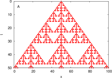
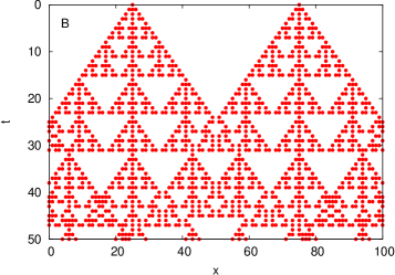
Figure 13: Solutions of the “partial BDE” (34): (a) for a single nonzero site at $t=0$; and (b) the collision of two “waves,” each originating from such a site. For the space and time steps $\theta_{z}=\theta_{t}=1$, this BDE is equivalent to the elementary cellular automaton (ECA) with rule 150; empty sites ($u_{i}(j)=0$) in white and occupied sites ($u_{i}(j)=1$) in black.

We notice that the system’s dynamics for any initial state of the pure Cauchy problem can be obtained from the evolution of the corresponding ECA that starts from initial data with a single nonzero value, which we show in Fig. 13a. This property of solutions is due to the fact that rule 150 exhibits the important simplifying feature of “additive superposition” [40], as evident from Fig. 13b, where the collision of two “waves” is plotted; this feature is the result of linearity (mod 2), as discussed in [2, 3] and in Sect. 2 here.

In the IBVP case, the solutions can behave quite differently, depending on the value of $N$ and on the initial state. We report here only the results for the IBVP with periodic initial data $u_{i}(0)=u_{i+T_{z}}(0)$ and number of variables $2N+1$, with $N$ chosen to be an integer multiple of the $space$ period $T_{z}$. In this case — apart from the presence of possible fixed points, in particular for $T_{z}\leq 3$ — the solutions of Eq. (34) display the longest $time$ periods when $T_{z}=N$. More precisely, $u_{0}(0)=u_{T_{z}}(0)=1$ and $u_{i}(0)=0$ for $i$ not a multiple of $T_{z}$; this choice of the initial state has the longest-possible $space$ period at fixed size $N$.

In agreement with other known results for ECA 150 [40, 118], we find that our solutions with $T_{z}=N$ are immediately $time$ periodic for $N$ not a multiple of three, whereas there is a transient when $N=3p,p\in\mathbb{N}$; this transient is of length 1 for $N$ odd and of length $2^{j-1}$, where $2^{j}$ is the largest power of two which divides $N$, otherwise. The ECA with rule 150 belongs to the third class in Wolfram’s classification [40, 41], in which evolution for $N\to\infty$ can lead to aperiodic, chaotic patterns. While the behavior of this ECA is predictable from the knowledge of the initial state for the IBVP with finite $N$, the length of the time period $T_{z}$ can increase rapidly with $N$. In particular, one finds a time period already as long as $511$ for space-periodic initial data with $T_{z}=N=19$.

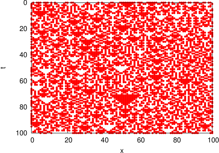
Figure 14: The solution of the BDE (34) starting from a random initial state of length $N=100$. The qualitative behavior is characterized by “triangles” of empty ($u_{i}(j)=0$) or occupied ($u_{i}(j)=1$) sites but without any recurrent pattern; this behavior does not depend on the particular random initial state.

To show that the behavior of the IBVP for Eq. (33) is not periodic in time in the limit of $N\rightarrow\infty$, we present in Fig. 14 the results for a random initial state of length $N=100$. These results do not show any “recurrent pattern,” apart from the expected [11, 43] appearance of characteristic “triangles” that still emerge from the chaotic distribution of empty and occupied sites.

We have seen in Sect. 2 (see Definition 2.1) that ordinary BDEs are conservative if their behavior is immediately periodic for any initial data, and that correspondingly they are also time-reversible. Our findings show that Eq. (33) is dissipative, since one observes transients for the periodic IBVP with various $N$ values; this is expected from its equivalence with the “parabolic” BDE (30). Nevertheless, in the ordinary BDE context, the connectives of the form (33), based on the $\bigtriangledown$ operator, are often conservative at least for some set of distinct delays. We wish therefore to extend the analysis of this partial BDE —from the case of all delays being equal, $\theta_{ij}\equiv\theta_{t}$, as above— to the case of distinct $\theta_{t}$ values in the rhs of Eq. (34), since this could lead to conservative behavior and to increasingly complex solutions for some set of delays. Doing so, however, goes beyond the purpose of the present paper and will have to await future work.

Another attempt at formulating parabolic partial BDEs is given by the equations:

$$u(z,t) = [u(z-\theta_{z},t-\theta_{t})\lor u(z+\theta_{z},t-\theta_{t})]\bigtriangledown u(z,t-\theta_{t}),$$ (35)

$$u(z,t) = [u(z-\theta_{z},t-\theta_{t})\wedge u(z+\theta_{z},t-\theta_{t})]\bigtriangledown u(z,t-\theta_{t}),$$ (36)

obtained from the parabolic PDE (28) by replacing $\partial_{zz}$ with the OR and the AND operator, respectively. From the known results on ordinary BDEs, the solutions in these cases can be expected to reproduce closely the behavior of dissipative PDEs. This intuitive conjecture is confirmed by the analysis in terms of their ECA equivalent. Thus, Eq. (35) corresponds to rule 54, in the first class, and Eq. (36) to rule 108, in the second class. Accordingly, the evolution of their solutions leads to fixed points or to small-period limit cycles, respectively; in neither case does the $N\rightarrow\infty$ limit display chaotic behavior. We thus expect these connectives to be good candidates as simple examples of “correct” partial BDE equivalents of dissipative PDEs.

5.4 Summary on partial BDEs and future work

Our results on classifying finite BDE systems, on the one hand, and our replacing partial derivatives in PDEs by Boolean operators, on the other, seem to provide interesting insights into the correspondence between partial BDEs and PDEs. In Sects. 5.1–5.3 we have only considered relatively easy cases, in which close correspondence exists between our partial BDEs and ECAs. This correspondence sheds new light on the known results of certain cellular automata.

We summarize our results on partial BDEs in Table 2. In the degenerate case of all delays being equal, $\theta_{ij}\equiv\theta_{t}$ for all $i$ and $j$, partial BDEs are always equivalent to particular CAs in the limit of infinite size, and their expected behavior can be obtained from the analogy. We gave examples of dissipative partial BDEs corresponding to ECAs in different classes of Wolfram’s classification [11]. In particular, a first-order approximation of the spatial derivative in the parabolic PDE (28), as well as a second-order approximation of this derivative in the hyperbolic PDE (27) yielded the same partial BDE (33), equivalent to ECA 150, which can behave very differently depending on the starting data. On the other hand, Eq. (29) gave immediately periodic solutions for all the starting data; hence this partial BDE is conservative. In the binary string formulation reviewed in Sect. 5.3, it corresponds to ECA rule 170, which is among the “forbidden” rules of Wolfram [11] because it describes asymmetric interactions. Given its simplicity, though, Eq. (29) and hence rule 170 seem perfectly legitimate in the present context.

More difficult situations, such as the case of nonconstant starting data in the initial interval, are left for future studies. To give an idea of the possible outcomes, consider the solution of Eq. (31) with initial data of the Riemann type, with a single jump in $u_{0}(z,t)$ at $z=0$ and $t_{0}=1/2<\theta_{t}$, i.e., $u_{0}(z,t)=1$ for $-\infty<z\leq 0$ and $0\leq t\leq 1/2$, and $u_{0}(z,t)=0$ in the rest of the initial strip, $\left\{(z,t):\,0<z<\infty,\>t<\theta_{t}\right\}\bigcup\left\{(z,t):-\infty<z\leq 0,\>1/2<t<\theta_{t}\right\}$. An obvious conjecture is that the solution will still be a right- or left-traveling wave, depending on the sign taken in the rhs of the partial BDE. More generally, certain $z$-periodic IBVPs will also be well posed and, in the more intriguing case of Eq. (33), additive superposition will provide insight into solution behavior, which might include certain solutions that exhibit both $z$- and $t$-periodicity.

In the parabolic partial BDE (35) we conjecture instead that the solution $u\equiv 1$ will be asymptotically stable, even for rationally independent $\theta_{z}$ and $\theta_{t}$ and nonconstant initial data, at least for large $|z|$. Conversely, $u\equiv 0$ should be asymptotically stable when replacing the OR operator by AND as in Eq. (36); see Theorem 2.9 in Sect. 2.5. However, nontrivial solutions of parabolic problems could be obtained in the presence of time-constant or time-periodic forcing, like for PDEs.

One further step would consist of looking at the same connectives with different delays, i.e. different $\theta_{t}$ values in the variables in the rhs of the equations. This should in particular allow one to better understand the classification of partial BDEs into conservative and dissipative, possibly depending on the open set of delays under consideration. We conjecture, moreover, that —for distinct, irrationally related delays— connectives similar to the one in Eq. (33) could have solutions of increasing complexity. If so, this would provide us with an even richer metaphor for evolution than either ordinary BDEs or ECAs.

6 What Next?

The most promising development in the theory and applications of BDEs seems to be the extension to an infinite, or very large, number of variables as discussed in Sect. 4 ($n\approx 10^{3}$) and Sect. 5 ($n\to\infty$). Inhomogeneous partial BDEs can be easily handled by introducing “variable coefficients,” i.e. multiplication of the right-hand side by site-dependent Boolean variables or functions.

Another important possibility is the randomization of various aspects of the BDE formulation. Wright et al. [119] have already considered ensemble averaging over BDE solutions with randomized initial data, while Zaliapin et al. [7, 8] have considered random forcing. It would be even more interesting to consider the random perturbation of delays, first in ordinary and then in partial BDEs; see also work along these lines in Boolean networks [58].

Next, an important but harder goal of the theory will be to develop inverse methods. In other words, given the behavior of a complicated natural system, which can be described in a first approximation by a finite number of discrete variables, one would like to discover a good connective linking these variables and yielding the observed behavior for plausible values of the delays. In this generality, the inverse problem for ODEs, say, is clearly intractable. But some of the direct results obtained so far — see, for instance, the asymptotic-simplification results in Sect. 2.5 — hold promise for BDEs, at least within certain classes and with certain additional conditions. Intuitively, the behavior of BDEs, although surprisingly rich, is more rigidly constrained than that of flows. Certain inverse-modeling successes have also been reported for cellular automata; see [11] and references there.

From the point of view of applications, BDEs have been applied fairly extensively by now to climate dynamics [4, 62, 63, 119, 120, 121, 122] and are making significant inroads into solid-earth geophysics [7, 8]. Most interesting are recent applications to the life sciences (Neumann and Weisbuch [123, 124], Gagneur and Casari [13], Öktem et al. [59]), which represent in a sense a return to the motivation of the geneticist René Thomas, originator of kinetic logic [20, 38, 39]; see also Sect. 2.6 and Appendix A for details.

BDEs may be suited for the exploration of poorly understood phenomena in the socio-economic realm as well. Moreover, the robustness of fairly regular solutions in a wide class of BDEs, for many sets of delays and a variety of initial states, suggests interesting applications to certain issues in massively parallel computations.

Acknowledgements. It is a pleasure to thank the organizers of the International Workshop and Seminar “Dynamics on Complex Networks and Applications” (DYONET 2006), especially Jürgen Kurths, for the opportunity to interact with the participants, as well as with the members of the Max-Planck-Institut für Physik Komplexer Systeme in Dresden, Germany, and prepare this research-and-review paper. We are indebted to all the collaborators who helped us formulate, analyze, and apply BDEs: D. P. Dee, V. I. Keilis-Borok, A. P. Mullhaupt, P. Pestiaux, and A. Saunders. Comments and suggestions by E. Simonnet and G. Weisbuch have helped improve the original manuscript. This work was supported by NSF Grant ATM-0327558, by the European Commission’s Project no. 12975 (NEST) ”Extreme Events: Causes and Consequences (E2-C2),” and by the ”Réseau francilien de recherche sur le développement soutenable (R2D2)” of the Région Ile-de-France.

Appendix A: BDEs and Kinetic Logic

A mathematical model closely related to BDEs was formulated by R. Thomas [38, 39] in a slightly different form. The difference can best be explained in terms of “memorization variables” $x_{ij}(t)=x_{j}(t-\theta_{ij})$. In our formulation $x_{ij}(t)$ is a purely delayed state variable; that is, $x_{ij}(t)$ is determined only by the state of the system at time $t-\theta_{ij}$. Thomas allows the memorization variable $x_{ij}(t)$ to depend on the state of the system up to and including time $t$: when a change takes place in any variable $x_{k}$ in the time interval $(t-\theta_{ij},t)$, then the memorization variable $x_{ij}$ may change as well.

Specifically, if for some $t^{\prime}\in(t-\theta_{ij},t)$ the state of the system is such that

$$x_{j}(t^{\prime})=f_{j}(x_{1}(t^{\prime}),\dots,x_{n}(t^{\prime}))\neq x_{j}(t-\theta_{ij}),$$ (37)

then the memorization variable $x_{ij}(t)$, previously equal to $x_{j}(t-\theta_{ij})$, is changed to

$$x_{ij}(t)=x_{j}(t^{\prime}).$$ (38)

The adjustment of the variables $x_{ij}$ is in effect selectively erasing some of the memory of the system. The resulting solutions are usually simpler and hence easier to study than the typical solution of our BDEs. Referring to the examples shown in Figs. 2 and 3 here, the increasing complexity of the solution reflects the fact that the memory of the system contains more and more information as time goes on.

In Thomas’s kinetic-logic formulation, such solutions of increasing complexity cannot arise. They are due precisely to the “conflicts” between variable values that were avoided on purpose in kinetic logic [13]. Some recent work on Boolean networks [58, 59] use a similar policy of eliminating behavior that appears to be too complicated, at least for certain purposes, and thus too hard to capture numerically. Eliminating the selective memory erasure of Eqs. (37) and (38) seems, on the other hand, to provide a cleaner, richer and more versatile mathematical theory [1, 2, 3].

Table 1. Common Boolean operators

Mathematical	Engineering	Name	Description
symbol	symbol
$\overline{x}$	NOT $x$	negator	not true when $x$ is true
$x\vee y$	$x$ OR $y$	logical or	true when either $x$ or $y$ or both are true
$x\wedge y$	$x$ AND $y$	logical and	$x\wedge y\equiv\overline{(\overline{x}\vee\overline{y})}$
$x\bigtriangledown y$	$x$ XOR $y$	exclusive or	true only when $x$ and $y$ are not equal
$x\bigtriangleup y$			true only when $x$ and $y$ are equal

PDE	Approxim-	PBDE	ECA	ECA	Eq. $n^{0}$ and
$\partial_{t}v=$	ation	$u_{i}(t+\theta_{t})=$	rule	class	behavior
$\partial_{z}v$	$\bigtriangledown$ (1st order)	$u_{i-1}(t)$	170	—	(29) C
$\partial_{zz}v$	$\vee$	$[u_{i-1}(t)\vee u_{i+1}(t)]\bigtriangledown u_{i}(t)$	54	I	(35) D
$\partial_{zz}v$	$\wedge$	$[u_{i-1}(t)\wedge u_{i+1}(t)]\bigtriangledown u_{i}(t)$	108	II	(36) D
$\partial_{zz}v$	$\bigtriangledown$ (1st order)
		$[u_{i-1}(t)\bigtriangledown u_{i+1}(t)]\bigtriangledown u_{i}(t)$	150	III	(33) D
$\partial_{z}v$	$\bigtriangledown$ (2nd order)

Summary of results on the partial BDEs (PBDEs) obtained from different approximations for the spatial derivative in the simplest parabolic and hyperbolic PDEs. The temporal derivative is always approximated to first order by the $\bigtriangledown$ operator. The last column gives the equation number and the behavior of the solutions, conservative (C) or dissipative (D). Notice that, though all but Eq. (29) in this table are dissipative, it is only Eq. (33) that displays chaotic behavior in the limit of infinite lattice size.

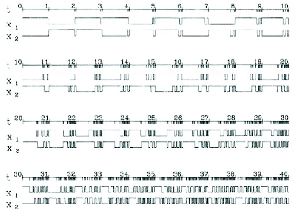
Figure 2: Solutions of the system of two conservative BDEs (6) for the delay $\theta=0.977$ and $0\leq t<40$ [1]. The tick marks on the $t$-axis indicate the times at which jumps in either $x_{1}$ or $x_{2}$ take place. After Dee and Ghil [1]. Copyright ©Society for Industrial and Applied Mathematics; reprinted with permission.

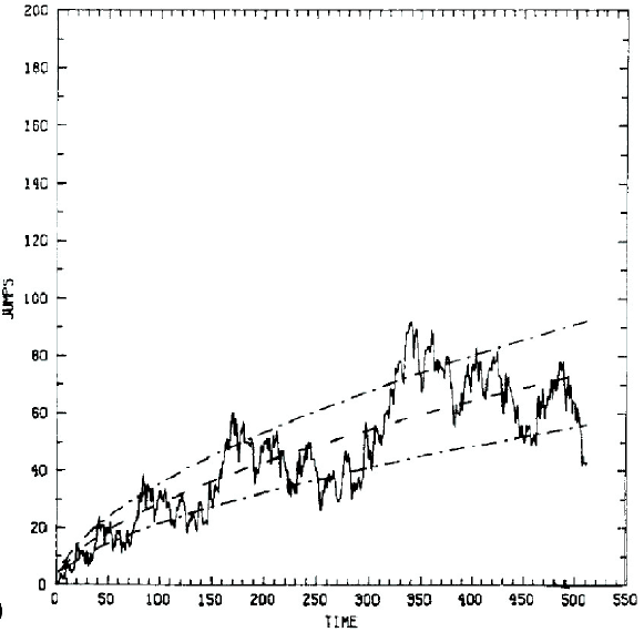
Figure 3: Jump function $J(t)$ for the particular solution of a conservative BDE with the irrational delay $\theta=(\sqrt{5}-1)/2$; see Eq. (9) and further details in the text. Reproduced from [3], with kind permission of Springer Science and Business Media.

Figure 7: Three seismic regimes in a colliding-cascade model of lithospheric dynamics; each earthquake sequence illustrates characteristic features of the corresponding regime and only a small fraction of each sequence is shown. Top panel – regime H (High), $\Delta_{H}=0.5\cdot 10^{4}$; middle panel – regime I (Intermittent), $\Delta_{H}=10^{3}$; bottom panel – regime L (Low), $\Delta_{H}=0.5\cdot 10^{3}$; in all three panels $\Delta_{L}=0.5\cdot 10^{4}$ (see also Fig. 10 below) and the number of nodes in the simulated lattice is $1093$, for a tree depth of $L=6$, the maximum magnitude of any earthquake in the BDE model. Reproduced from Zaliapin et al. [7], with kind permission of Springer Science and Business Media.

References

- [1] Dee D., and M. Ghil, 1984. Boolean difference equations, I: Formulation and dynamic behavior. SIAM J. Appl. Math. 44, 111–126.
- [2] Mullhaupt, A. P., 1984. Boolean Delay Equations: A Class of Semi-Discrete Dynamical Systems. Ph. D. thesis, New York University [published also as Courant Institute of Mathematical Sciences Report CI-7-84, 193 pp.]
- [3] Ghil, M., and A. P. Mullhaupt, 1985. Boolean delay equations. II: Periodic and aperiodic solutions. J. Stat. Phys. 41, 125–173.
- [4] Ghil, M., A. P. Mullhaupt, and P. Pestiaux, 1987. Deep water formation and Quaternary glaciations. Clim. Dyn. 2, 1–10.
- [5] Ghil, M., and A. W. Robertson, 2000. Solving problems with GCMs: General circulation models and their role in the climate modeling hierarchy. In D. Randall (Ed.) General Circulation Model Development: Past, Present and Future, Academic Press, San Diego, pp. 285–325.
- [6] Saunders, A., and M. Ghil, 2001. A Boolean delay equation model of ENSO variability. Physica D 160, 54–78.
- [7] Zaliapin, I., V. Keilis-Borok, and M. Ghil, 2003a. A Boolean delay equation model of colliding cascades. Part I: Multiple seismic regimes. J. Stat. Phys. 111, 815–837.
- [8] Zaliapin, I., V. Keilis-Borok, and M. Ghil, 2003b. A Boolean delay equation model of colliding cascades. Part II: Prediction of critical transitions. J. Stat. Phys. 111, 839–861.
- [9] Cowan, G. A., D. Pines and D. Melzer, Eds., 1994. Complexity: Metaphors, Models and Reality. Addison-Wesley, Reading, Mass, 705 pp.
- [10] Gutowitz, H., 1991. Cellular Automata: Theory and Experiment. MIT Press, Cambridge, MA, 485 pp.
- [11] Wolfram, S., 1994. Cellular Automata and Complexity: Collected Papers. Addison-Wesley, Reading, Mass, 610 pp.
- [12] Kauffman, S. A., 1995. At Home in the Universe: The Search for Laws of Self-Organization and Complexity. Oxford University Press, New York, 338 pp.
- [13] Gagneur, J., and G. Casari, 2005. From molecular networks to qualitative cell behavior. FEBS Letters 579 (8), Special Issue, 1867–1871.
- [14] Arnol’d, V. I., 1983. Geometrical Methods in the Theory of Ordinary Differential Equations. Springer-Verlag, New York, 376 pp.
- [15] Smale, S., 1967. Differentiable dynamical systems. Bull. Amer. Math. Soc. 73, 747–817.
- [16] Collet, P., and J.-P. Eckmann, 1980. Iterated Maps on the Interval as Dynamical Systems. Birkhäuser Verlag, Basel/Boston/Birkhäuser, 264 pp.
- [17] Hénon, M., 1966. La topologie des lignes de courant dans un cas particulier. C. R. Acad. Sci. Paris 262, 312–414.
- [18] von Neumann, J., 1966. Theory of Self-Reproducing Automata, University of Illinois Press, Urbana, Illinois, 388 pp.
- [19] Kauffman, S.A., 1993. The Origins of Order: Self-Organization and Selection in Evolution, Oxford University Press, USA, 734 pp.
- [20] Thomas, R., Ed., 1979. Kinetic Logic: A Boolean Approach to the Analysis of Complex Regulatory Systems, Springer-Verlag, Berlin/Heidelberg/New York, 507 pp.
- [21] Arnold B. H., 1962. Logic and Boolean Algebra. Prentice-Hall, Englewood Cliffs, New Jersey, 144 pp.
- [22] Bhattacharrya, K. and M. Ghil, 1982. Internal variability of an energy-balance model with delayed albedo effects. J. Atmos. Sci. 39, 1747–1773.
- [23] Driver, R. D., 1977. Ordinary and Delay Differential Equations, Applied Mathematical Sciences Series, 20, Springer-Verlag, New York.
- [24] Hale, J., 1971. Functional Differential Equations. Springer-Verlag, New York, 238 pp.
- [25] McDonald, N., 1978. Time Lags in Biological Models. Springer-Verlag, New York, 112 pp.
- [26] Bellman, R. and K. L. Cooke, 1963. Differential-Difference Equations. Academic Press, New York.
- [27] Isaacson, E. and H. B. Keller, 1966. Analysis of Numerical Methods. John Wiley, New York.
- [28] Guckenheimer, J., and P. Holmes, 1997. Nonlinear Oscillations, Dynamical Systems and Bifurcations of Vector Fields. 3rd ed, Springer-Verlag, New York, 475 pp.
- [29] Lichtenberg, A. J., and M. A. Liebermann, 1992. Regular and Chaotic Dynamics, 2nd ed., Springer-Verlag, New York, 714 pp.
- [30] Lorenz, E. N., 1963. Deterministic nonperiodic flow. J. Atmos. Sci. 20, 130–141.
- [31] Arnol’d, V. I., 1978. Mathematical Methods of Classical Mechanics, Springer-Verlag, New York, 462 pp.
- [32] Varadi, F., B. Runnegar, and M. Ghil, 2003. Successive refinements in long-term integrations of planetary orbits. Astrophys. J. 592, 620–630.
- [33] Ghil, M., and S. Childress, 1987. Topics in Geophysical Fluid Dynamics: Atmospheric Dynamics, Dynamo Theory and Climate Dynamics, Springer-Verlag, New York/Berlin/London/Paris/Tokyo, 485 pp.
- [34] Dijkstra, H. A., and M. Ghil, 2005. Low-frequency variability of the large-scale ocean circulation: A dynamical system approach. Rev. Geophys. 43, RG3002, doi:10.1029/2002RG000122.
- [35] Khinchin, A. Ya., 1964. Continued Fractions, Univ. of Chicago Press, Chicago, IL.
- [36] Andronov, A. and L. Pontryagin, 1937. Systèmes grossiers. Dokl. Akad. Nauk. USSR 14, 247–251.
- [37] Jacob, F. and J. Monod, 1961. Genetic regulatory mechanisms in the synthesis of proteins. J. Mol. Biol. 3, 318–356.
- [38] Thomas, R., 1973. Boolean formalization of genetic control circuits. J. theor. Biol. 42, 563–585.
- [39] Thomas, R., 1978. Logical analysis of systems comprising feedback loops. J. theor. Biol. 73, 631–656.
- [40] Wolfram, S., 1983. Statistical-mechanics of cellular automata. Rev. Mod. Phys. 55, 601–644; also included in [11].
- [41] Wolfram, S., 1984. Universality and complexity in cellular automata. Physica D 10, 1–7; also included in [11].
- [42] Kauffman, S. A., 1969. Metabolic stability and epigenesis in randomly constructed genetic nets. J. theor. Biol. 22, 437–467.
- [43] Weisbuch, G., 1991. Complex Systems Dynamics: An Introduction to Automata Networks. Lecture Notes Volume II, Santa Fe Institute, Studies in the Sciences of Complexity. Addison Wesley, Redwood City, CA, 208 pp.
- [44] Derrida, B., and Y. Pomeau, 1986. Random networks of automata: A simple annealed approximation. Europhys. Lett. 1, 45–49.
- [45] Derrida, B., and G. Weisbuch, 1986. Evolution of overlaps between configurations in random Boolean networks. J. Physique 47, 1297–1303.
- [46] Varadi, F., M. Ghil and W. M. Kaula, 1999. Jupiter, Saturn and the edge of chaos. Icarus 139, 286–294.
- [47] Correale, L., M. Leone, A. Pagnani, M. Weigt, and R. Zecchina, 2006. Core percolation and onset of complexity in Boolean networks, Phys. Rev. Lett. 96, 018101-1–018101-4.
- [48] Correale, L., M. Leone, A. Pagnani, M. Weigt, and R. Zecchina, 2006. Computational core and fixed-point organisation in Boolean networks, J. Stat. Mech. P03002.
- [49] Mézard, M., G. Parisi, and R. Zecchina, 2002. Analytic and algorithmic solution of satisfiability problems, Science 297, 812–815.
- [50] Albert, R., and A.-L. Barabási, 2002. Statistical mechanics of complex networks, Rev. Mod. Phys. 74, 47–97.
- [51] Kauffman, S., C. Peterson, B. Samuelsson, and C. Troein, 2004. Genetic networks with canalyzing Boolean rules are always stable. Proc. Natl. Acad. Sci. USA 101, 17102–17107.
- [52] Mesot, B., and C. Teuscher, 2005. Deducing local rules for solving global tasks with random Boolean networks. Physica D 211, 88–106.
- [53] Samuelsson, B., and C. Troein, 2003. Optimization of robustness and connectivity in complex networks. Phys. Rev. Lett. 90, 068701-1–068701-4.
- [54] Drossel, B., T. Mihaljev, and F. Greil, 2005. Scaling in critical random Boolean networks. Phys. Rev. Lett. 94, 088701-1–088701-4.
- [55] Mihaljev, T., and B. Drossel, 2006. Scaling in a general class of critical random Boolean networks, Phys. Rev. E 74, 046101-1–046101-10.
- [56] Gershenson, C., 2004. Introduction to random Boolean networks, nlin.AO/0408006. in Bedau, M., P. Husbands, T. Hutton, S. Kumar and H. Suzuchi (eds.) Workshop and Tutorial Proceeding, Ninth International Conference on the Simulation and Synthesis of Living Systems (ALife IX), 160–173.
- [57] Gershenson, C., 2002. Classification of random Boolean networks. In Standish, R. K., M. A. Bedau and H. A. Abbass (eds), Artificial Life VIII: Proceedings of the Eight International Conference on Artificial Life, pp 1–8, MIT Press.
- [58] Klemm, K., and S. Bornholdt, 2005. Stable and unstable attractors in Boolean networks. Phys. Rev. E 72, 055101-1–055101-4.
- [59] Öktem, H., R. Pearson, and K. Egiazarian, 2003. An adjustable aperiodic model class of genomic interactions using continuous time Boolean networks (Boolean delay equations). Chaos 13, 1167–1174.
- [60] Gabrielov, A., V. Keilis-Borok, I. Zaliapin, and W. I. Newman, 2000. Critical transitions in colliding cascades, Phys. Rev. E 62, 237–249.
- [61] Gabrielov, A. M., I. V. Zaliapin, V. I. Keilis-Borok, and W. I. Newman, 2000. Colliding cascades model for earthquake prediction. J. Geophys. Intl. 143, 427–437.
- [62] Darby, M. S., and L. A. Mysak, 1993. A Boolean delay equation model of an interdecadal Arctic climate cycle. Clim. Dyn. 8, 241–246.
- [63] Wohlleben, T. M. H. and A. J. Weaver, 1995. Interdecadal climate variability in the subpolar North Atlantic. Clim. Dyn. 11, 459–467.
- [64] Diaz, H. F., and V. Markgraf, Eds., 1993. El Niño: Historical and Paleoclimatic Aspects of the Southern Oscillation. Cambridge Univ. Press, New York, 490 pp.
- [65] Philander, S. G. H., 1990. El Niño, La Niña, and the Southern Oscillation, Academic Press, San Diego, 312 pp.
- [66] Glantz, M. H., R. W. Katz, and N. Nicholls, Eds. 1991. Teleconnections Linking Worldwide Climate Anomalies. Cambridge Univ. Press, New York, 545 pp.
- [67] Maraun, D., and J. Kurths, 2005. Epochs of phase coherence between El Niño/Southern Oscillation and Indian monsoon. Geophys. Res. Lett. 25, 171–174.
- [68] Latif, M., T. P. Barnett, M. Flügel, N. E. Graham, J.-S. Xu, and S. E. Zebiak, 1994. A review of ENSO prediction studies. Clim. Dyn. 9, 167–179.
- [69] Ghil, M., and N. Jiang, 1998. Recent forecast skill for the El Niño/Southern Oscillation. Geophys. Res. Lett. 25, 171–174.
- [70] Bjerknes, J., 1969, Atmospheric teleconnections from the equatorial Pacific. Mon. Wea. Rev. 97, 163–172.
- [71] Chang, P., B. Wang, T. Li, and L. Ji, 1994. Interactions between the seasonal cycle and the Southern Oscillation: Frequency entrainment and chaos in intermediate coupled ocean-atmosphere model. Geophys. Res. Lett. 21, 2817–2820.
- [72] Chang, P., L. Ji, B. Wang, and T. Li, 1995. Interactions between the seasonal cycle and El Niño - Southern Oscillation in an intermediate coupled ocean-atmosphere model. J. Atmos. Sci. 52, 2353–2372.
- [73] Jin, F.-f., J. D. Neelin, and M. Ghil, 1994. El Niño on the Devil’s Staircase: Annual subharmonic steps to chaos, Science 264, 70–72.
- [74] Jin, F.-f., J. D. Neelin, and M. Ghil, 1996. El Niño/Southern Oscillation and the annual cycle: Subharmonic frequency locking and aperiodicity, Physica D 98, 442–465.
- [75] Tziperman, E., L. Stone, M. A. Cane, and H. Jarosh, 1994. El Niño chaos: Overlapping of resonances between the seasonal cycle and the Pacific ocean-atmosphere oscillator. Science 264, 72–74.
- [76] Tziperman, E., M. A. Cane, and S. E. Zebiak, 1995. Irregularity and locking to the seasonal cycle in an ENSO prediction model as explained by the quasi-periodicity route to chaos. J. Atmos. Sci. 50, 293–306.
- [77] Battisti, D. S., 1988. The dynamics and thermodynamics of a warming event in a coupled tropical atmosphere/ocean model. J. Atmos. Sci. 45, 2889–2919.
- [78] Dijkstra, H. A., 2005. Nonlinear Physical Oceanography: A Dynamical Systems Approach to the Large Scale Ocean Circulation and El Niño. 2nd ed, Springer, New York, 532 pp.
- [79] Neelin, J. D., M. Latif, and F.-f. Jin, 1994. Dynamics of coupled ocean-atmosphere models: the tropical problem. Annu. Rev. Fluid Mech. 26, 617–659.
- [80] Jin, F.-f., 1996. Tropical ocean-atmosphere interaction, the Pacific cold tongue, and the El-Niño-Southern Oscillation. Science 274, 76–78.
- [81] Jin F.-f., and J. D. Neelin, 1993. Modes of interannual tropical ocean-atmosphere interaction – A unified view. I. Numerical results. J. Atmos. Sci. 50, 3477–3503.
- [82] Jin, F.-f., and J. D. Neelin, 1993. Modes of interannual tropical ocean-atmosphere interaction – A unified view. II. Analytical results in fully coupled cases. J. Atmos. Sci. 50, 3504–3522.
- [83] Jin, F.-f., and J. D. Neelin, 1993. Modes of interannual tropical ocean-atmosphere interaction – A unified view. III. Analytical results in fully coupled cases. J. Atmos. Sci. 50, 3523–3540.
- [84] Jensen, M. H., P. Bak, and T. Bohr, 1984. Transition to chaos by interaction of resonances in dissipative systems. Part I. Circle maps. Phys. Rev. A 30, 1960–1969.
- [85] Schuster, H. G., 1988. Deterministic Chaos: An Introduction. Physik-Verlag, Weinheim.
- [86] Mandelbrot, B. 1982. The Fractal Geometry of Nature. W. H. Freeman, New York, 480 pp.
- [87] Peitgen, H.-O., and P. Richter, 1986. The Beauty of Fractals, Springer-Verlag, Heidelberg, 211 pp.
- [88] Peitgen, H., H. Jürgens and D. Saupe, 1992. Chaos and Fractals: New Frontiers of Science, Springer-Verlag, New York.
- [89] Rasmusson, E. M., X. Wang, and C. F. Ropelewski, 1990. The biennial component of ENSO variability. J. Marine Syst. 1, 71–96.
- [90] Jiang, N., J. D. Neelin and M. Ghil, 1995. Quasi-quadrennial and quasi-biennial variability in the equatorial Pacific. Clim. Dyn. 12, 101–112.
- [91] Moron, V., R. Vautard, and M. Ghil, 1998. Trends, interdecadal and interannual oscillations in global sea-surface temperatures, Clim. Dyn. 14, 545–569.
- [92] Yiou, P., D. Sornette, and M. Ghil, 2000. Data-adaptive wavelets and multi-scale SSA, Physica D 142, 254–290.
- [93] Burridge, R., and L. Knopoff, 1967. Model and theoretical seismicity, Bull. Seism. Soc. Am. 57, 341–371.
- [94] Allègre, C. J., J. L. Le Mouel, and A. Provost, 1982. Scaling rules in rock fracture and possible implications for earthquake prediction. Nature 297, 47–49.
- [95] Bak, P., C. Tang, and K. Wiesenfeld, 1988. Self-organized criticality. Phys. Rev. A 38, 364–374.
- [96] Keilis-Borok, V. I., 2002. Earthquake prediction: State-of-the-art and emerging possibilities. Annu. Rev. Earth Planet. Sci. 30, 1–33.
- [97] Keilis-Borok, V. I. and P. N. Shebalin, Eds., 1999. Dynamics of lithosphere and earthquake prediction. Phys. Earth Planet. Int. 111, 179–330.
- [98] Newman, W. I., A. M. Gabrielov, and D. L. Turcotte, Eds., 1994. Nonlinear Dynamics and Predictability of Geophysical Phenomena, Geophys. Monographs Ser. 83, American Geophysical Union, Washington, DC, 107 pp.
- [99] Rundle, J. B., D. L. Turcotte, and W. Klein, Eds., 2000. Geocomplexity and the Physics of Earthquakes. American Geophysical Union, Washington, DC, 284 pp.
- [100] Turcotte, D. L., W. I. Newman, and A. M. Gabrielov, 2000. A statistical physics approach to earthquakes. In: J. B. Rundle, D. L. Turcotte, and W. Klein, Eds., Geocomplexity and the Physics of Earthquakes. American Geophysical Union, Washington, DC, pp. 83–96.
- [101] Keilis-Borok, V. I., 1996. Intermediate-term earthquake prediction. Proc. Natl. Acad. Sci. USA 93, 3748–3755.
- [102] Scholz, C. H., 2002. The Mechanics of Earthquakes and Faulting, 2nd ed., Cambridge University Press, Cambridge, 496 pp.
- [103] Turcotte, D. L., 1997. Fractals and Chaos in Geology and Geophysics, 2nd ed., Cambridge University Press, Cambridge, 412 pp.
- [104] Press, A. and C. Allen, 1995. Pattern of seismic release in the southern California region. J. Geophys. Res. 100, 6421–6430.
- [105] Romanowicz, B., 1993. Spatiotemporal patterns in the energy-release of great earthquakes, Science 260, 1923–1926.
- [106] Mertins, A., 1999. Signal Analysis: Wavelets, Filter Banks, Time-Frequency Transforms and Applications. John Wiley and Sons, Chichester, 330 pp.
- [107] Keilis-Borok, V. I. and L. N. Malinovskaya, 1964. One regularity in the occurrence of strong earthquakes. J. Geophys. Res. 69, 3019–3024.
- [108] Jaume S. C., and L. R. Sykes, 1999. Evolving towards a critical point: A review of accelerating seismic moment/energy release prior to large and great earthquakes, Pure Appl. Geophys. 155, 279–306.
- [109] Keilis-Borok, V. I., 1994. Symptoms of instability in a system of earthquake-prone faults, Physica D 77, 193–199.
- [110] Pepke, G. F., J. R. Carlson, and B. E. Shaw, 1994. Prediction of large events on a dynamical model of fault. J. Geophys. Res. 99, 6769–6788.
- [111] Molchan, G. M., O. E. Dmitrieva, I. M. Rotwain, and J. Dewey, 1990. Statistical analysis of the results of earthquake prediction, based on burst of aftershocks. Phys. Earth Planet. Int. 61, 128–139.
- [112] Knopoff, L., T. Levshina, V. I. Keilis-Borok, and C. Mattoni, 1996. Increased long-range intermediate-magnitude earthquake activity prior to strong earthquakes in California. J. Geophys. Res. 101, 5779–5796.
- [113] Bufe, C. G. and D. J. Varnes, 1993. Predictive modeling of the seismic cycle of the Greater San Francisco Bay region. J. Geophys. Res. 98, 9871–9883.
- [114] Bowman, D. D., G. Ouillon, C. G. Sammis, A. Somette, and D. Sornette, 1998. An observational test of the critical earthquake concept. J. Geophys. Res. 103, 24359–24372.
- [115] Courant, R., and D. Hilbert, 1962. Methods of Mathematical Physics. Vol. II, Wiley-Interscience, New York/London/Sydney, 830 pp.
- [116] Richtmyer, R. D., and K. W. Morton, 1967. Difference Methods for Initial-Value Problems, Wiley, New York (2nd ed), 420 pp.
- [117] Van Leer, B., 1979. Towards the ultimate conservation difference scheme. V. A second order sequel to Godunov’s method. J. Comput. Phys. 32, 101–135.
- [118] Martin, O., A. M. Odlyzko and S. Wolfram, 1984. Algebraic properties of cellular automata. Comm. Math. Phys. 93, 219-258; also included in [11].
- [119] Wright, D. G., T. F. Stocker, and L. A. Mysak, 1990. A note on Quaternary climate modelling using Boolean delay equations. Clim. Dyn. 4, 263–267.
- [120] Nicolis, C., 1982. Boolean approach to climate dynamics. Q. J. R. Meteorol. Soc. 108, 707–715.
- [121] Mysak, L. A., D. K. Manak, and R. F. Marsden, 1990. Sea-ice anomalies observed in the Greenland and Labrador Seas during 1901–1984 and their relation to an interdecadal Arctic climate cycle. Clim. Dyn. 5, 111–113.
- [122] Kellogg, W. W., 1983. Feedback mechanisms in the climate system affecting future levels of carbon dioxide. J. Geophys. Res. 88, 1263–1269.
- [123] Neumann, A. and G. Weisbuch, 1992. Window automata analysis of population dynamics in the immune system. Bull. Math. Biol. 54, 21–44.
- [124] Neumann, A. and G. Weisbuch, 1992. Dynamics and topology of idiotypic networks. Bull. Math. Biol. 54, 699–726.