Predictability of El Niño as a Nonlinear Stochastic Limit Cycle

Abstract

Abstract: The El Niño phenomenon, synonymously El Niño-Southern Oscillation (ENSO), is an anomalous climatic oscillation in the Equatorial Pacific that occurs once every 3-8 years. It affects the earth’s climate on a global scale. Whether it is a cyclic or a sporadic event, or whether its apparently random behaviour can be explained by stochastic dynamics have remained matters of debate. Herein ENSO is viewed, unconventionally, as a two-dimensional dynamical system on a desktop. The main features of ENSO: irregularity, interannual variability, and the asymmetry between El Niño and La Niña are captured, simply, comprehensibly, quickly and cheaply, in a nonlinear stochastic limit cycle paradigm. Its predictability for ENSO compares remarkably well with that of the best state-of-the-art complex models from the European and American meteorological centres. Additionally, for the first time, by analyzing subsurface Equatorial Pacific data since 1960, this model finds that long-term variations are not caused by ENSO itself, but by external sources.

Keywords: El Niño-Southern Oscillation (ENSO), stochastic limit cycle, recharge oscillator, Niño3, thermocline depth

Royal Netherlands Meteorological Institute (KNMI), Postbus 201, 3730 AE De Bilt, The Netherlands

El Niño is an anomalous climatic event in the Equatorial Pacific. On average, the western Pacific sea-surface temperature (SST) is about $4^{\circ}$-$5^{\circ}$C higher than that of the eastern Pacific, and the thermocline, or the sharp vertical temperature gradient separating the warm and the cold water, lies deeper in the western Pacific than in the Eastern Pacific. The higher SST of the western Pacific results in rising warm, moist air from the Indonesian coast, and the descent of cool, dry air towards the eastern south Pacific. These atmospheric movements are supplemented by the high altitude eastward jet stream and the westward trade winds along the Equatorial Pacific sea surface. During an El Niño, which peaks in the northern winter, the eastern Pacific gets warmer as the pool of warm water stretches much further eastward. The western Pacific thermocline becomes shallower and the westward trade winds at the sea surface become much weaker, and sometimes even reverse. These anomaly conditions in the Equatorial Pacific affect the earth’s climate at a global scale.

That ENSO is a result of ocean-atmosphere interaction has been clear since the time of Bjerknesbjerknes . It has been well-established that there are three key players in the ocean-atmosphere interaction that determine the ENSO dynamics at interannual time-scales: the SST, the atmospheric wind stress anomaly and the ocean’s ability to transport energyphilander in the Equatorial Pacific. However, how the dynamics of these quantities relate to each other to perturb the normal climatic conditions to create an El Niño, and especially how the growth of an El Niño is controlled so that the normalcy is restored have remained matters of discussion.neelinrev A large number of models geared to address these issues — ranging from dynamical models inspired by the physics of ENSOphilanderpap ; hirst ; cane1 ; zebiak ; battistialone ; suarez ; graham ; battisti ; neelin1 ; wang ; jin3 ; vaart ; neelin2 to stochastic onesphilander2 ; lau ; burgers1 ; neelin ; jin0 ; eckert ; kleeman ; tziperman ; flugel ; penland ; tahl — have put forward different mechanisms at varying degrees of complexity: for some ENSO is inherently unstablephilanderpap ; hirst and the nonlinearities in ENSO dynamics eventually control the growth of an El Niñocane1 ; zebiak ; battistialone ; suarez ; graham ; battisti , while some others have assumed that the normal climatic condition is stable and that ENSO is excited by noisewang ; philander2 ; jin3 ; lau ; neelin ; eckert ; kleeman ; tziperman ; flugel ; penland ; tahl . These models have also differed in their interpretation of the role of noise originating from external processes at a faster time scale, and the role of nonlinearity in ENSO properties. Over and above, they can capture different features of ENSO in their own ways; nevertheless, the ability to reproduce all the basic features of ENSO, while being able to simultaneously predict ENSO with good accuracy in a comprehensive manner is still lacking in the ENSO model worldneelinrev . Remarkably, one such feature of ENSO not easily reproduced is the skewness of the ENSO indices, or the asymmetry between El Niño and La Niñasteph .

Given this setting, herein ENSO is viewed, unconventionally, as a two-dimensional dynamical system on a desktop, described by the Niño3 index, the anomaly in the average SST of the region $5^{\circ}$S-$5^{\circ}$N, $150^{\circ}$W-$90^{\circ}$W, and the anomaly in Z$20$ or the average depth of the $20^{\circ}$C isotherm (as a proxy for the thermocline depth) of the region $5^{\circ}$S-$5^{\circ}$N, $120^{\circ}$E-$290^{\circ}$E, henceforth denoted by $T$ and $H$ respectively. Using the Niño3 and Z20 data averaged over month $i$, the (discrete) ENSO dynamical system indexed by $(T_{i},H_{i})$ is constructed. Based on the physics of ENSO, a phenomenological model, subject to fixed-amplitude Gaussian white noise, is conjectured to describe this dynamical system. The model captures, simply, comprehensibly, quickly and cheaply, all the main features of ENSO: irregularity, interannual variability, and the asymmetry between El Niño and La Niña, in a nonlinear stochastic limit cycle paradigm. Its predictability for ENSO compares remarkably well with that of the best state-of-the-art complex models from the European and American meteorological centres. Additionally, for the first time, by analyzing subsurface Equatorial Pacific (Z20) data since 1960 (roughly the time when regular record-keeping of subsurface Pacific temperature profile began), this model finds that decadal (and above) variations stem from external sources, e.g. climate shifts.

ENSO as a nonlinear stochastic limit cycle

The idea behind viewing ENSO as a two-dimensional dynamical system is based on the so-called “recharge oscillator”jin1 ; jin2 ; jin3 , which identifies the Equatorial eastern Pacific SST anomaly $T_{E}$, the equatorial eastern and the western Pacific thermocline depth anomalies $H_{E}$ and $H_{W}$, and the central Pacific zonal wind-stress anomaly $\tau$ as the main oceanic and atmospheric quantities involved in the ENSO dynamics. The Equatorial eastern and the western Pacific thermocline depth anomalies can be combined to form two independent variables: $(H_{E}-H_{W})$, representing the “thermocline anomaly tilt”, and $(H_{E}+H_{W})$, representing the anomaly in the amount of warm water volume present in the Equatorial Pacific (WWVA)jin1 ; jin2 ; jin3 ; kessler ; meinen2 . Of these two, a positive anomaly in $(H_{E}-H_{W})$ is strongly in phase with a positive eastern Pacific SST anomaly and a positive central Pacific zonal wind-stress anomaly. As envisaged by the recharge oscillator, before the onset of an El Niño, (meridional) Sverdrup transport of warm water towards the Equator gives rise to a positive anomaly in the WWVA. A positive WWVA gives rise to a positive $T_{E}$. Subsequently, $\tau$ responds positively to a positive $T_{E}$, and increases $(H_{E}-H_{W})$. These changes in the Pacific surface conditions then generate Rossby and Kelvin thermocline waves in the equatorial waveguide: these waves first make the western Pacific thermoclines shallower, and the return of the reflected waves at the western Pacific boundaries, further on, reduces the eastern Pacific SST anomaly.

The recharge oscillator does not explain how the (meridional) Sverdrup transport of warm water towards (or away from) the Equator is triggered. Nonetheless, it seems logical that a positive WWVA results in a positive $T_{E}$ and vice versa. A linear relationship between these two quantities was conjectured by Burgers et al.jin3 , but that is in contradiction with the observation data: the magnitude of the positive $T_{E}$ due to a given positive magnitude of the WWVA during an El Niño is larger than the magnitude of $T_{E}$ due to a negative WWVA of the same magnitude during a La Niñameinen2 ; mcphadden . This asymmetry between the El Niño and the La Niña (manifested equivalently via the Niño3 skewnesssteph ), not fully understood at present, indicate that how the WWVA and $T_{E}$ interact is unclear: scenarios based on air-sea fluxes feedback on the SST, and the oceanic upwelling and vertical mixing mechanism have been suspected to contribute to itwang1 ; wang2 . The fact however remains that the WWVA leads $(H_{E}-H_{W})$, $T_{E}$ and $\tau$, which are strongly in phase with each other, by approximately 7 months on average, and consequently it should be considered as an important predictor for $T_{E}$ at ENSO time-scales. The natural variables in the (minimalistic) model for ENSO herein, therefore, are the Niño3 monthly anomaly as a representative of $T_{E}$, and the Z20 monthly anomaly, representing the WWVA (hereafter denoted by $T$ and $H$ respectively), forming a two-dimensional dynamical system. The lack of our understanding of how the WWVA and $T_{E}$ interact motivated this study of ENSO as a stochastic dynamical system, based on empirical data.

The monthly Niño3 and Z20 anomalies in dimensionless units (rendered dimensionless by normalizing w.r.t. their r.m.s. magnitudes), hereafter denoted by $(t,h)$, are shown in Fig. 1. A positive $t$ (resp. $h$) means a positive Niño3 anomaly (resp. WWVA) and vice versa. In this notation, the aim of this study is to describe the ENSO dynamics stochastically as $t_{i+1}=f(t_{i},h_{i})+\xi_{i},h_{i+1}=g(t_{i},h_{i})+\eta_{i}$, where $f(x,y)$ and $g(x,y)$ are two nonlinear functions of their arguments, and $\xi$ and $\eta$ are mutually uncorrelated fixed-amplitude Gaussian white noise. Visual inspection of the data in Fig. 1 suggests strong locking of the ENSO dynamics to its phase [defined by $\phi=-\tan^{-1}(h/t)$], and therefore a cylindrical co-ordinate system $r=\sqrt{t^{2}+h^{2}}$ and $\phi$, is more suitable. In these co-ordinates, without any loss of generality, the nonlinearities in the ENSO dynamics are then expressed by two coupled nonlinear differential equations as: $dr/dt\equiv r\gamma(r,\phi)$ and $d\phi/dt\equiv\omega(r,\phi)$, with the $(r_{i},\phi_{i})$-values obtained from the corresponding $(t_{i},h_{i})$ ones.

Figure 1: (a) Normalized monthly anomaly data for Niño3 ($t$) and Z20 ($h$) in the Equatorial Pacific, describing ENSO for 1980-2004 (source: MET office objective analysis for the ENSEMBLES project, hereafter referred to as the “ENSEMBLES data”; publicly available at http://www.ecmwf.int/research/EU_projects/ENACT/ocean_analyses/index.html); (b) The same for the 1980-2002 data obtained from Australian Bureau of Meteorology (hereafter ABOM); publicly available at http://www.bom.gov.au/bmrc/ocean/results/climocan.htm#subsurface%20anals].

Based on the resemblance of Fig. 1 to a limit cycle (i.e., a tendency to grow when the system is close to $r=0$, combined with a tendency to decay when the system grows far away form $r=0$) strongly locked to its phase, the ansatz $\gamma(r,\phi)=f_{1}(\phi)[f_{2}(\phi)-r]$ and $\omega(r,\phi)=g_{1}(\phi)\sqrt{r}$ is made to describe ENSO. It is clear from Fig. 1 that $f_{2}(\phi)$ cannot simply be a constant, and for an explanation for $\omega(r,\phi)\propto\sqrt{r}$ see the methods section. With this ansatz, the natural choice for $f_{1}(\phi)$, $f_{2}(\phi)$ and $g_{1}(\phi)$ is clearly a series expansion in increasing orders of sines and cosine harmonics as $(A+B_{1}\cos\phi+B_{2}\sin\phi+C_{1}\cos 2\phi+C_{2}\sin 2\phi+\ldots)$. The parameters $A,B_{1},B_{2},\ldots$ can then be estimated from a time-series $(t_{i},h_{i})$. This estimation is performed in the following manner: the observed time-series for $N$ sequential months were denoted as $(t_{1},h_{1})$, $(t_{2},h_{2})$, $\ldots,(t_{N},h_{N})$. Then for $i=1,2\ldots N$, $(t_{i},h_{i})$ is taken as the starting value and $dr/dt$ and $d\phi/dt$ are integrated forward from time $i$ to time $(i+1)$ using the functional forms of $\gamma(r,\phi)$ and $\omega(r,\phi)$. This yields the model theoretical values $(\tilde{t}_{i+1},\tilde{h}_{i+1})$, as well as the noise ${\mathbf{e}}_{i}=(t_{i+1}-\tilde{t}_{i+1},h_{i+1}-\tilde{h}_{i+1})$. The parameters $A,B_{1},B_{2},\ldots$ can then be estimated by least-square optimization, i.e., by minimizing $E=\sum_{i=1}^{N-1}{\mathbf{e}}_{i}\cdot{\mathbf{e}}_{i}$. Note that this optimization process not only yields the parameter values, but also the characteristics of the noise ${\mathbf{e}}_{i}$, to be later used to realistically construct $\xi$ and $\eta$.

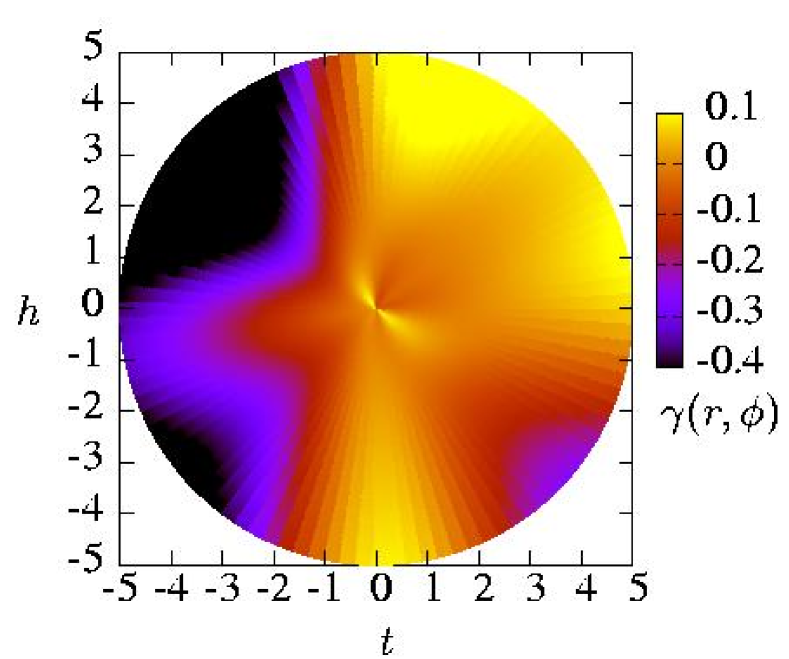
Figure 2: Phase-space manifold structure for the ENSO dynamics, given by $dr/dt$ and $d\phi/dt$, in terms of $\gamma(r,\phi)$ and $\omega(r,\phi)$.The parameters that generated these plots have been optimized on the 1980-2004 $(t,h)$ ENSEMBLES data [Fig. 1(a)]. The corresponding phase-space manifold structure for the ABOM data (not shown here) of Fig. 1(b) is only marginally different from the above, as it should be; this confirms the stability of the optimization process to describe ENSO.

To fix the functional forms for $f_{1}(\phi)$, $f_{2}(\phi)$ and $g(\phi)$ that are to be used throughout the entire length of this study, ABOM data [Fig. 1(b)] were used for the least-square optimization. To capture the annual variations of $t$ and $h$, any choice of $f_{1}(\phi)$, $f_{2}(\phi)$ and $g(\phi)$ needed to include the fourth harmonics for the sine and cosine functions (on average, ENSO has a 4-year period); and simultaneously, due to the finiteness of the time-series, the number of parameters in $\gamma(\phi)$ and $\omega(\phi)$ have been kept as low as possible. Eventually, the functional forms of $f_{1}(\phi)$, $f_{2}(\phi)$ and $g(\phi)$ that used the smallest number of parameters while still leading to the smallest value of $E$ for the Australian dataset were chosen. This procedure showed that there are $16$ parameters needed to describe $f_{1}(\phi)$, $f_{2}(\phi)$ and $g(\phi)$ [or $\gamma(r,\phi)$ and $\omega(r,\phi)$]. See the methods section for details.

As it turns out, the ansatz about the functional forms for $\gamma(r,\phi)$ and $\omega(r,\phi)$ are very well-chosen. One of its immediate outcomes is that the noise characteristics that emerged from Fig. 1 can be fairly accurately described as Gaussian white. The rest of the outcomes: “stability” of this method, ENSO irregularity, variability, Niño3 skewness and predictability are discussed below.

Stability of the optimization procedure

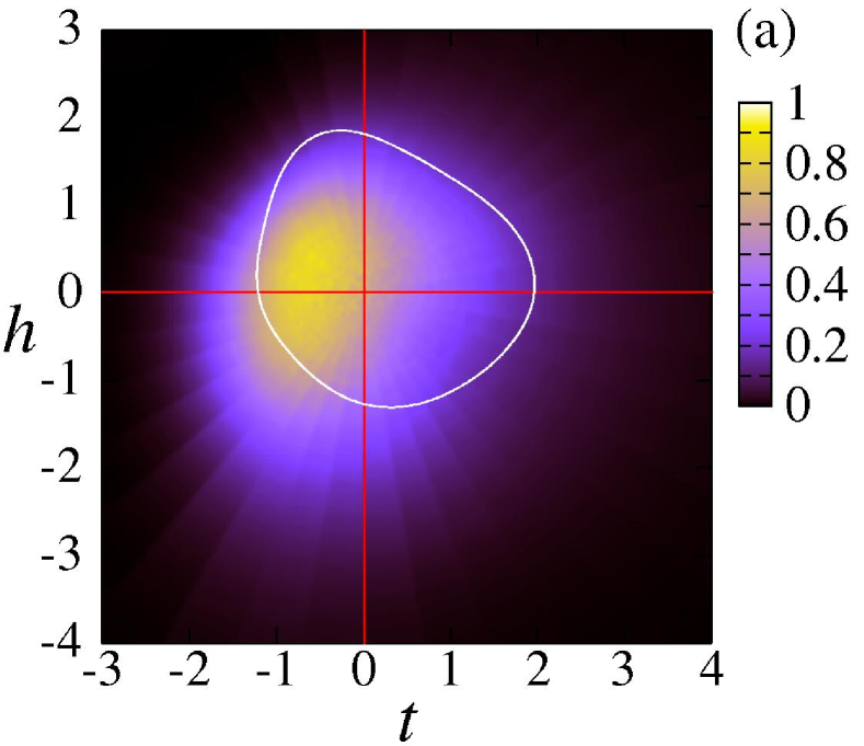
Figure 3: (a): Probability density for finding an ENSO state at $(t,h)$ in colour plot. The white closed curve is the average path (obtained by averaging the locations of all data points within $10^{\circ}\,\phi$-intervals for the $5,000,000$ year run) of ENSO as a stochastic limit cycle. It implies that on average an initial ENSO state inside the white curve evolves in time to converge to it from inside, while an initial ENSO state outside the white curve evolves in time to converge to it from outside. The resemblance of Fig. 3(a) to Fig. 1(a) or (b) is clear. Note the relation of the white curve to the WWVA anomaly at the onset of an El Niño: a sharp positive anomaly in Equatorial WWVA precedes an El Niño, which is nicely captured by the hump in the white curve in the $(t<0,h>0)$ quadrant. (b) Probability density $P(s)$ of skewness $s$ of the Niño3 index, calculated from $200,000$ sets of $25$ years each (obtained from the same $5,000,000$ year run). The Niño3 skewness based on the $25$ year UK MET office objective analysis data (1980-2004) appearing in Fig. 1(a) is approximately $0.85$, while the average Niño3 skewness obtained from Fig. 3(b) is $0.81$. The broad probability distribution of the Niño3 skewness exemplifies the extent of ENSO variability within the scope of this model. These plots use the same values for the parameters as in Fig. 2.

The first issue for describing ENSO by means of these $16$-parameter functional forms for $\gamma(r,\phi)$ and $\omega(r,\phi)$ is the “stability” of the optimization procedure; namely that all the major ENSO features: irregularity, variability and Niño3 skewness are expected to be properly reproduced when the same minimization procedure is applied to a dataset reasonably similar to the ABOM one. The noise characteristics emerging from that new dataset are also expected to appear to be sufficiently close to Gaussian white. To this end the ENSEMBLES data [Fig. 1(a)] were used, and both expectations were fulfilled. Not only did the phase-space manifold structure of ENSO dynamics show clear signatures of growth and decay in the ENSO magnitude $r$ [see Figs. 2(a) and (b)], but also when the corresponding parameters were used, in addition to Gaussian white noise (of strength obtained from the minimization procedure; see methods section), to simulate the two-dimensional stochastic dynamical system version of ENSO on a computer for $5,000,000$ years, it produced the right 1980-2004 ENSO features. Two of these are shown in Fig. 3. In Fig. 3(a) appears the probability density function for finding the ENSO state at $(t,h)$ in colour plot. The white closed curve is the average path (obtained by averaging the locations of all data points within $10^{\circ}\,\phi$-intervals for the $5,000,000$ year run) of ENSO as a stochastic limit cycle. It implies that on average an initial ENSO state inside the white curve evolves in time to converge to it from inside, while an initial ENSO state outside the white curve evolves in time to converge to it from outside. The resemblance of Fig. 3(a) to Fig. 1(a) or (b), which prompted the ansatz to model ENSO as a limit cycle in the first place, is clear. Also clear is the relation of the white curve to the WWVA anomaly at the onset of an El Niño: a sharp positive anomaly in Equatorial WWVA precedes an El Niñomeinen2 ; wang1 ; wang2 , which is nicely captured by the hump in the white curve in the $(t<0,h>0)$ quadrant. Simultaneously, Fig. 3(b) shows the probability density $P(s)$ of skewness $s$ of the Niño3 index, calculated from $200,000$ sets of $25$ years each (obtained from the same $5,000,000$ year run). The skewness of the Niño3 index based on the $25$ year (1980-2004) ENSEMBLES data appearing in Fig. 1(a) is approximately $0.85$, while the average Niño3 skewness obtained from Fig. 3(b) is $0.81$. The broad probability distribution of the Niño3 skewness exemplifies the extent of ENSO variability within the scope of this model.

Predictability skill

The ultimate test of how robustly ENSO can be described by a two-dimensional stochastic dynamical system as above is to be able to predict ENSO with a reasonable accuracy. In order to address this issue, predictability for Niño3 over the period $1960$-now was studied by running a 10,000 different sequences of Gaussian white noise realizations in this model, using the ENSEMBLES data (available up to $1960$, roughly when records-keeping of reliable regular subsurface Pacific temperature profile began). It is to be emphasized here that (a) The use of subsurface Equatorial Pacific data to analyze the relation between WWVA and ENSO has so far dated back to $1980$. This study, therefore, is the first one to extend that to pre-$1980$; (b) This model’s predictability for Niño3 has been studied thoroughly by considering a wide variety of “training periods”, i.e., the periods from which the data are used to optimize the parameters of the model. The results presented here are based on the training period 1980-2004 as described below; this choice is motivated as it also sheds light on the role of climate shifts on ENSO; and (c) Unless otherwise stated, in order to avoid artificial skill, the target period has never been included in the training period.

Figure 4: Comparison between the predicted average (red) and the observed (blue) values of normalized Niño3 monthly anomalies over the period $1960$-now (and beyond): lead time $3$ months (top) and $6$ months (bottom). The yellow areas show the $2\sigma$-spread in the $3$- and $6$-month lead time predictions (they also give a general idea about the magnitude of the $2\sigma$-spread over the $1960$-June $2006$ period), based upon runs of 10,000 realizations. See methods section for details.

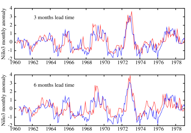
Figure 6: Comparison between predicted (red) and unfiltered observation data (blue) for Niño3 monthly anomaly over 1960-1979. The uniform gap of nearly 1^∘C between the two curves before 1976 is due to the well-known 1976-shift. This gap disappears (Fig. 4 in the paper) when the observation data is passed through a high-pass filter that removes decadal (and above) variations in Niño3 and Z20.

The predictability skill results (see methods section for the calculations and the convention for lead time) for the years $1960$-now appear in Fig. 4. The underlying subtleties can be broken down to three separate periods. (i) $1980$-$2004$: In order to make sure that the training period of the model did not include any information from the “target dataset”, i.e., the dataset corresponding to the year for which Niño3 is to be predicted, the so-called “jackknifing” procedure was used. More explicitly, the $(t,h)$ normalized anomaly dataset was first formed out of the $1979$-$2004$ Niño3 and Z20 monthly averages. Next, for the predictions of year $n$ ($1980\leq n\leq 2004$), the data for the years $n-1$, $n$ and $n+1$ were removed from the $(t,h)$ dataset of 1979-2004 to form a jackknived dataset, which served as the training period for the model. (ii) $1960$-$1979$: Two separate normalized anomaly datasets $(t,h)$ were formed, one out of the Niño3 and Z20 monthly averages of $1960$-$2004$ data, and the other out of the $1980$-$2004$ data. The target dataset was formed by truncating the former to $1960$-$1979$, while the training period for the model was $1980$-$2004$. The comparison between the corresponding predicted and observed $t$-values for the years $1960$-$1979$ revealed a startling gap between the two (see Fig. 6 in Appendix D), as if the predicted magnitudes of Niño3 were uniformly shifted upwards by approximately $1^{\circ}$C compared to the observed ones over the period 1960-1976. Interestingly, when the Niño3 and Z20 anomaly values for $1960$-$2004$ were first passed through a high-pass filter that removed the variations in these variables at time-scales $\geq 10$ years, and were subsequently normalized and truncated to $1960$-$1980$ in order to form the target dataset, the uniform gap between the predicted and observed Niño3 values disappeared (this is the comparison shown in Fig. 4). Upon further reflection, it was understood that this uniform gap corresponds to the well-known climatological shift in $1976$ (known as the “1976-shift”trenberth ). Interpreted differently, the disappearance of the gap between predicted and filtered observation data indicates that variations in the Equatorial Pacific climatic conditions ENSO have two distinct components in it: climatological shifts (i.e., shifts in the mean background) that occur due to dynamics at decadal (or above) time-scales and variations that occur at ENSO time-scales. It is the latter kind of variations that are captured by the stochastic limit cycle picture. The issues related to the origin of decadal variations in ENSO do remain matters of discussionfedorov ; flugel1 ; rodgers ; yeh ; schopf1 ; nevertheless, the conclusions of this analysis contradicts the view that climatological shifts of ENSO are a part of its own dynamics. (iii) $2005$-now (and beyond): The climatological means and normalizations for the target dataset $(t,h)$ as well as the training period for the model is $1980$-$2004$.

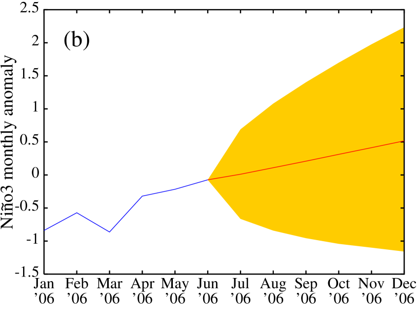
Figure 5: (a) Predictability skill of this model for $1960$-June $2006$ (i.e., correlations between the red and blue curves of Fig. 4). See also Fig. 8 in Appendix D for skill as a function of months. (b) Niño3 monthly anomaly for 2006, based upon the climatology of $1980$-$2004$; observation (blue); predicted average (red). The yellow area shows the $2\sigma$-spread.

Finally, the predictability skill, i.e., Niño3 monthly anomaly correlations between observation and average of Niño3 anomaly (as they appear in Fig. 4) for $1960$-June 2006 are shown in Fig. 5(a). The predictions until December 2006, as obtained by (iii) above appear in Fig. 5(b).

Skill comparison with operational models

The comparison of the predictability skill of this model with the four highest-ranked operational models [System-2 (S2)stockdale coupled atmosphere-ocean model from European meteorological centre ECMWF, and Constructed Analogue (CA)dool1 ; dool2 , Markovxue and Climate Forecast System (CFS)saha from the U.S. centre for meteorology NCEP] for the period $1987$-$2001$ are presented in Table I. It provides a fair yardstick for the predictability power of this model. Since different strategies were used in different models to generate ensembles and the number of members varied over the period $1987$-$2001$, making this comparison has not been entirely trivial. Nevertheless, the period $1987$-$2001$ is actually selected as it is the common denominator of these operational modelsgj . See also Fig. 8 in Appendix D for skill comparisons as a function of months.

	lead months
model	$\quad\,2\quad\quad\quad\quad\quad\,4\quad\quad\quad\quad\quad\,\,6$	training/tuning period
S2	$0.94\quad\quad\quad\quad 0.87\quad\quad\quad\quad 0.76$	$\quad\quad\,\,1987$-$2001$
Markov	$0.87\quad\quad\quad\quad 0.75\quad\quad\quad\quad 0.63$	$\quad\quad\,\,1981$-$1995$
CA	$0.83\quad\quad\quad\quad 0.76\quad\quad\quad\quad 0.70$	$\quad\quad\,\,1956$-$2001$
CFS	$0.89\quad\quad\quad\quad 0.80\quad\quad\quad\quad 0.71$	$\quad\quad\,\,1987$-$2001$
This model	$0.90\quad\quad\quad\quad 0.79\quad\quad\quad\quad 0.69$	$\quad\quad\,\,1960$-$2004$

Table I: Comparison of the prediction skill of this dynamical systems model with the best operational models [S2 from ECMWF, and CA, Markov and CFS from NCEP] for the period $1987$-$2001$. The CA and Markov models are statistical, and the CFS and S2 models are coupled atmosphere-ocean general circulation model (AO-GCM). Over this period, the two-dimensional dynamical system model used here performs slightly better than those of the NCEP statistical ones, and slightly worse than the AO-GCM of ECMWF. Source: van Oldenborgh et al., 2003gj .

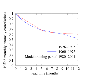
Figure 9: Predictability skill of the dynamical systems model in the paper. This figure is meant for comparison with Fig. 2 of Chen et al. (2004). To generate this figure, the decadal (and above) variations have been removed from the 1960-1979 dataset, as discussed in the “Predictability skill” section of the paper.

It is also worth noting that a relatively recent work by Chen et al.chen , using training period $1980$-$2000$anderson reported that large El Niños could be predicted up to two years in advance. A predictability comparison with that work before $1960$ is not possible because of the lack of Z20 data. Nevertheless, when the training period $1980$-$2004$ is used, the model discussed in this paper produces very similar skills on target periods $1960$-$1975$ and on $1976$-$1995$ (Fig. 9 in Appendix D).

Conclusion

The idea behind viewing ENSO as a two-dimensional stochastic dynamical system in this work has been based on the recharge oscillator formulation. In this formulation, essentially the amount of warm water in the Equatorial Pacific controls ENSO. Although it is clear that a larger amount of warm water volume in the Equatorial Pacific results in a higher eastern Pacific SST and vice versa, how these two quantities interact is far from clear; a fact that this study draws its motivation from. It considers subsurface Pacific data roughly since record-keeping of reliable regular subsurface Pacific temperature profile began (1960), for the first time. This simple model firmly establishes that a two-dimensional dynamical system, and more specifically, a nonlinear stochastic limit cycle captures the essentials of ENSO to a great detail, as it (i) captures the well-known features of ENSO comprehensively, (ii) is able to predict ENSO with an accuracy well-comparable with the state-of-the-art complex models from the European and American meteorological centres, and (iii) is able to separate the nature of decadal and multi-decadal variations from the interannual variability of ENSO. This development signifies the fact that oceanic upwelling, vertical layer mixing, and air-sea fluxes feedback mechanismswang1 ; wang2 should be paid more attention to in order to fully understand ENSO, as the interaction between the subsurface warm water volume and the SST takes place via these mechanisms. The expectation is that the parameters of this dynamical system are related to these mechanisms, and that remains a topic of future research.

Appendix A

0.1 Explanation for $\omega(r,\phi)\propto\sqrt{r}\,$:

This proportionality has been actually chosen (i) to avoid the ambiguity of defining $\omega(r,\phi)$ at $r=0$, (ii) as well as for “regularization”: should the system get stuck in a phase of uncontrolled growth, the $\sqrt{r}$ term serves to move it quickly away from there. In general, $\omega(r,\phi)\propto r^{n}$ for any $n>0$ can serve for both, so there is some arbitrariness in the choice of $n$. Nevertheless, $n=1/2$ was a choice motivated to keep the model as simple as possible: $n=0$ does not work for (i) and (ii), and $n=1$ was found to contradict the observation data, and hence the choice $n=1/2$ was made. It is also worthwhile to note that the results presented here are insensitive of the value of $n$ within the range $0.3\lesssim n\lesssim 0.8$.

Appendix B

0.2 Least-square optimization and the functional forms of $f_{1}(\phi)$, $f_{2}(\phi)$ and $g(\phi)\,$:

For given functional forms of $f_{1}(\phi)$, $f_{2}(\phi)$ and $g(\phi)$ parametrized by $n$ quantities (such as $A$, $B_{1}$ etc.), the least-square optimization is a minimization of the scalar function $E$ defined on an $n$-dimensional manifold. In order to perform this minimization the amoeba method was usedpress . To make sure that the true minimum for $E$ was reached, the minimization was started from a multitude of initial values of the $n$ parameters. A single minimization run on $25$ years of monthly data takes about 15 minutes on a 1.8 GHz CPU. For the $1980$-$2002$ $(t,h)$ ABOM data initial trial minimization runs were set up with $f_{1}(\phi)=a_{0}+(b_{01}\cos\phi+c_{01}\sin\phi)+\ldots+(b_{04}\cos 4\phi+c_{04}\sin 4\phi)$, $f_{2}(\phi)=1+b_{1}\cos\phi+c_{1}\sin\phi$, and $g(\phi)=a_{2}+(b_{21}\cos\phi+c_{21}\sin\phi)+\ldots+(b_{24}\cos 4\phi+c_{24}\sin 4\phi)$. It was found that increasing the number of parameters beyond $16$ hardly reduced the minimum value of $E$. Once the number of parameters was thus fixed at $16$, more trials were run with different combinations of sine and cosine harmonics. Eventually, for the ABOM data, it was found that the forms of $f_{1}(\phi)$, $f_{2}(\phi)$ and $g(\phi)$ that lead to the minimum value of $E$ are the following: $f_{1}(\phi)=a_{0}+b_{01}\cos\phi+b_{02}\cos 2\phi+c_{02}\sin 2\phi+b_{03}\cos 3(\phi-\phi_{03})+b_{04}\cos 4(\phi-\phi_{03}/2)$, $f_{2}(\phi)=1+b_{1}\cos\phi+c_{1}\sin\phi$, and $g(\phi)=a_{2}+b_{21}\cos\phi+c_{21}\sin\phi+b_{21}\cos 2\phi+c_{21}\sin 2\phi+b_{23}\cos 3\phi+b_{24}\cos 4\phi$. These functional forms were used all throughout this study. The noise properties of obtained from these data were found to be Gaussian white to a good approximation.

For later references, note here that when these functional forms were used on the $1980$-$2004$ ENSEMBLES data [see Fig. 1(a)], the noise characteristics again turned out Gaussian white to a good approximation, with HWHM $0.34$ and $0.29$ for $t$ and $h$ respectively.

Appendix C

0.3 ENSO prediction as a function of lead months:

The predictability studies for ENSO were performed in the usual way: the numerical values of the model parameters were obtained from the $(t,h)$ data over the training period. These parameters were then used to time-evolve an initial state $(t_{0},h_{0})$ to $(t_{i},h_{i})$ for $i=1,\ldots,12$ using $10,000$ different sequences of Gaussian white noise realizations; this takes only about a minute on a 1.8 GHz CPU. The HWHM used for the Gaussian white noise were $0.34$ for $t$ and $0.29$ for $h$, as found from the optimization procedure on the ENSEMBLES data. The predicted $(t_{i},h_{i})$ values constitute the prediction for “lead time $i$ months”.

Appendix D

This appendix consists of additional figures to supplement the text.

Figure 7: Predictability skill of the dynamical system model as a function of target months for 1960-2006 (i.e., between the red and blue curves of Fig. 4).

Figure 8: Predictability skill of the dynamical system model in the paper as a function of target months. This figure is meant for comparison with Fig. 2 of van Oldenborgh et al. (2005), which shows the ENSO predictability skill for the operational models of Table I.

References

The authors wishe to thank Geert Jan van Oldenborgh, Wilco Hazeleger and Ruben Pasmanter for useful discussions and comments on the manuscript, and Bruce Ingleby at ECMWF and Sjoukje Philip for their help with the data.

References

- (1) Bjerknes J (1969) Atmospheric teleconnections from the Equatorial Pacific. Mon. Weather Rev. 97: 163–172.
- (2) Philander S G H (1990) El Niño, La Niña and the southern oscillation. Academic Press, San Diego, California.
- (3) Neelin J D (1998) et al. ENSO theory. J. Geophys. Res. 103: 14261–14290.
- (4) Philander S G H, Yamagata T, Pacanowski R C (1994) Unstable air-sea interactions in the tropics. J. Atmos. Sci. 41: 604–613.
- (5) Hirst A C (1986) Unstable and damped Eqatorial modes in simple coupled ocean-atmosphere models. J. Atmos. Sci. 43: 606–632.
- (6) Cane M A, Zebiak S E (1985) Theory for El Niño and Southern Oscillation. Science 228: 1085–1087.
- (7) Zebiak S E, Cane M A (1987) A model El Niño-Southern Oscillation. Mon. Weather Rev. 115: 2262–2278.
- (8) Battisti D S (1988) The dynamics and thermodynamics of a warming event in a coupled tropical atmosphere/ocean model. J. Atmos. Sci. 45: 2889–2919.
- (9) Suarez M J, Schopf P S (1988) A delayed action oscillator for ENSO. J. Atmos. Sci. 45: 3283–3287.
- (10) Graham N E, White W B (1988) The El Nino/Southern Oscillation as a natural oscillator of the tropical Pacific Ocean-Atmosphere system. Science 240: 1293–1302.
- (11) Battisti D S, Hirst A C (1989) Interannual variability in a tropical atmosphere-ocean system: Influence of the basic state, ocean geometry, and non-linearity. J. Atmos. Sci. 46: 1687–1712.
- (12) Van der Vaart P C F, Dijkstra H A, Jin F-F (2000) The Pacific cold tongue and the ENSO mode: unified theory within the Zebiak-Cane model. J. Atmos. Sci. 57: 967–988.
- (13) Neelin J D (1991) The slow sea surface temperature mode and the fast-wave limit: Analytic theory for tropical interannual oscillations and experiments in a hybrid coupled model. J. Atmos. Sci. 48: 584–606.
- (14) Neelin J D, Dijkstra H A (1995) Ocean-atmosphere interaction and the tropical climatology. Part I: The dangers of flux correction. J. Climate 8: 1325–1342.
- (15) Burgers G, Jin F-F, van Oldenborgh, G J (2005) The simplest ENSO recharge oscillator. Geophys. Res. Lett. 32: L13706.
- (16) Wang B, Fang Z (1996) Chaotic oscillations of tropical climate: A dynamical systems theory for ENSO. J. Atmos. Sci. 53: 2786–2802.
- (17) Philander S G H, Fedorov A (2003) Is El Niño sporadic or cyclic? Ann. Rev. Earth Planet. Sci. 31: 579-594.
- (18) Jin F-F, Neelin J D, Ghil M (1994) El Niño on a devil’s staircase: Annual subharmonic steps to chaos. Science 264: 70–72.
- (19) Burgers G (1999) El Niño stochastic oscillator. Clim. Dyn. 15: 521-531.
- (20) Neelin J D (1990) A hybrid coupled general circulation model for El Niño studies. J. Atmos. Sci. 47: 647–693.
- (21) Lau K-M (1985) Elements of stochastic dynamical theory of the long-term variability of the El Niño/Southern Oscillation. J. Atmos. Sci. 42: 1552–1558.
- (22) Eckert C, Latif M (1997) Predictability of a stochastically forced hybrid coupled model of El Niño. J. Climate 10: 1488–1504.
- (23) Kleeman R, Power S B (1994) Limits to predictability in a coupled ocean-atmosphere model due to atmospheric noise. Tellus 46A: 529–540.
- (24) Tziperman E et al. (1994) El Niño chaos: overlapping of resonances between the seasonal cycle and the Pacific ocean-atmosphere oscillator. Science 264: 72–74.
- (25) Flügel M, Chang P (1996) Impact of dynamical and stochastic processes on the predictability of ENSO. Geophys. Res. Lett. 23: 2089–2092.
- (26) Penland C, Sardeshmukh P D (1995) The optimal growth of tropical sea surface temperature anomalies. J. Climate 8: 1999–2024.
- (27) Kestin T S et al. (1998) Time-frequency variability of ENSO and stochastic simulations. J. Climate 11: 2258–2272.
- (28) Burgers G, Stephenson D B (1999) The “normality” of El Niño. Geophys. Res. Lett. 26, 1027–1030.
- (29) Jin F-F (1997) An equatorial recharge paradigm for ENSO, I, conceptual model. J. Atmos. Sci. 54: 811–829.
- (30) Jin F-F (1997) An equatorial recharge paradigm for ENSO, II, conceptual model. J. Atmos. Sci. 54: 830–847.
- (31) Kessler W S (2002) Is ENSO a cycle or a series of events?. Geophys. Res. Lett. 29: 2125.
- (32) Meinen C S, McPhaden M J (2000) Observations of warm water volume changes in the Equatorial Pacific and their relationship to El Niño and La Niña. J. Climate 13: 3551–3559.
- (33) McPhaden M J (2003) Tropical Pacific ocean heat content variatons and ENSO persistence barriers. Geophys. Res. Lett. 30: 1480.
- (34) Wang W, McPhadden M J (1999) The surface-layer heat balance in the Equatorial Pacific ocean. Part I: mean seasonal cycle. J. Phys. Oceanog. 29: 1812–1831.
- (35) Wang W, McPhadden M J (2000) The surface-layer heat balance in the Equatorial Pacific ocean. Part I: interannual variability. J. Phys. Oceanog. 30, 2989–3008.
- (36) Press W H et al. (1992) Numerical recipes in C: the art of scientific computing. (Cambridge University Press, New York.
- (37) Fedorov A V, Philander S G H (2001) A stability analysis of tropical ocean-atmospher interactions: Bridging measurements and theory for El Niño. J. Climate 14: 3086–3101.
- (38) Flügel M, Chang P, Penland C (2004) The role of stochastic forcing in modulating ENSO predictability. J. Climate 17: 3125–3140.
- (39) Rodgers K B, Firederichs P, Latif M (2004) Tropical Pacific decadal variability and its relation to decadal modulations of ENSO. J. Climate 17: 3761–3774.
- (40) Yeh S-W, Kirtman B P (2004) Tropical Pacific decadal variability and ENSO amplitude modulations in a CGCM. J. Geophys. Res. 109: C11009.
- (41) Schopf P S, Burgman R J (2006) A simple mechanism for ENSO residuals and asymmetry. J. Climate 19: 3167–3179.
- (42) Trenberth K E, Stepaniak D P (2001) Indices of El Niño evolution. J. Climate 14: 1697–1701.
- (43) Stockdale T N et al. (1998) Global seasonal rainfall forecast using a coupled ocean-atmosphere model. Nature 392: 370–373.
- (44) van den Dool H M (1994) Searching for analogues, how long must one wait? Tellus 46A: 314–324.
- (45) van den Dool H M, Barnston A G (1994) Forecast of global sea surface temperature out to a year using the Constructed Analogue method. In Proceedings of 19th Climate Diagnostics Workshop, pp. 416–419 (College Park, MD).
- (46) Xue Y A, Ji M (2000) ENSO prediction with Markov models: the impact of sea level. J. Climate 13: 849–871.
- (47) Saha S et al. (2006) The NCEP Climate Forecast System. J. Climate 19: 3843–3517.
- (48) van Oldenborgh G J et al. (2005) Did the ECMWF seasonal forecast model outperform statistical ENSO forecasts models over the last 15 years? J. Climate 18: 3240–3249.
- (49) Chen D et al. (2004) Predictability of El Niño over the past 148 years. Nature 428: 733–736.
- (50) Anderson D (2004) Testing time for El Niño. Nature 428: 709–711.