Geometric characterization of nodal domains: the area-to-perimeter ratio

Abstract

In an attempt to characterize the distribution of forms and shapes of nodal domains in wave functions, we define a geometric parameter - the ratio $\rho$ between the area of a domain and its perimeter, measured in units of the wavelength $1/\sqrt{E}$. We show that the distribution function $P(\rho)$ can distinguish between domains in which the classical dynamics is regular or chaotic. For separable surfaces, we compute the limiting distribution, and show that it is supported by an interval, which is independent of the properties of the surface. In systems which are chaotic, or in random-waves, the area-to-perimeter distribution has substantially different features which we study numerically. We compare the features of the distribution for chaotic wave functions with the predictions of the percolation model to find agreement, but only for nodal domains which are big with respect to the wavelength scale. This work is also closely related to, and provides a new point of view on isoperimetric inequalities.

1 Introduction

In this work we study the (real) eigenfunctions of the Laplace-Beltrami operator $-\Delta_{\mathcal{M}}$ on a Riemannian surface $\mathcal{M}$ with Dirichlet boundary conditions (if $\mathcal{M}$ has boundaries). Consider a real eigenfunction which satisfies

$$\left(\Delta_{\mathcal{M}}+E_{j}\right)\psi_{j}(r)=0\quad,\quad\left.\psi_{j}(r)\right|_{r\in\partial\mathcal{M}}=0\ .$$ (1)

The nodal domains are the maximally connected domains in $\mathcal{M}$ where $\psi_{j}$ has a constant sign. The nodal set (or the set of nodal lines) is the zero set: $U_{j}=\{r\in\mathcal{M}:\psi_{j}(r)=0\}$, which also forms the boundaries of the nodal domains. We shall denote the nodal count (i.e. the number of nodal domains) of $\psi_{j}(r)$ by $\nu_{j}$.
The investigation of quantum signatures of classical chaos and integrability has been a hot topic in quantum chaos for a long time [1, 2]. In the past few years, the interest in nodal domains, their counting and their morphology increased after Blum et al [3] proposed a quantitative method which distinguishes between the distributions of nodal counts in domains where the underlying classical dynamics is integrable (separable) or chaotic. This added a new approach, the statistical investigation of nodal patterns, to the more common investigation methods of spectral or wavefunction statistics, which are often connected to random-matrix theory [4]. Blum et al showed that if $\nu_{j}$ is the nodal count of the $j$th energy eigenstate of a domain , then $\xi_{j}=\nu_{j}/j$ has a limiting distribution $P(\xi)=\lim_{n\rightarrow\infty}\frac{1}{n}\sum_{j=1}^{n}\delta(\xi-\xi_{j})$ , where the characteristics of the distribution depend on the classical properties of the domain. For separable domains, $P(\xi)$ has a square root singularity at a (system-dependent) maximum value, while for chaotic systems $P(\xi)$ is (approximately) normally distributed. Comparison between the numerical results for chaotic billiards and the random-wave ensemble supports Berry’s conjecture [5] - wave functions in a chaotic system behave in the limit of high energy like a random superposition of plane waves. By that, the qualitative observation of Miller et al [6], that nodal sets can be used to distinguish between wave functions in chaotic and integrable domains, could be tested in a quantitative way. Other studies of various quantities - which pertain to the morphology and complexity of the nodal network - were published in the mathematical and physical literature, building upon the older results regarding the bounds on the total lengths of the nodal lines and their curvature [7, 8]. E.g., in [9] the distribution of the curvature is calculated, in addition to the mean and the variance of the total length of the nodal set. The distribution of the avoidance distances between nodal lines was also computed [10], to mention few examples.
An important breakthrough has been achieved by Bogomolny and Schmit [11] who implemented a critical percolation model that explains the large scale structure of nodal domains in chaotic wave functions. This model is supported by a variety of numerical calculations. For example: the expectation value and variance of the nodal count for chaotic billiards, as well as the distribution of areas of nodal domains, follow the predictions of the model [3, 11]; The nodal lines in the high energy limit seem (on large scales) to be SLE₆ curves [12, 13, 14] as it is proved for the boundaries of percolation clusters [15]. Despite the good agreement, the percolation description is a priori insensitive to the structure of the nodal set in scales of the order of a wavelength. In addition, it was demonstrated by Foltin et al [16] that there are some special measures with a scaling behavior which is different for percolation and the nodal set of the random-wave ensemble. The latter special measures, in general, probe subwavelength scales at two points at a (large) distance.

In this work we suggest a new (quantum mechanical) method for the classification of billiards according to their classical properties. We will discuss below in what sense the signatures in nodal patterns differ from the scenario known for the more common spectral and wavefunction analysis.
Our method provides yet another test to the conjectures by Berry and Bogomolny. The parameter which we use in order to interrogate the morphology of nodal lines is defined as follows - We consider the $j$th eigenfunction of (1), and its nodal domains sequence $\{\omega_{j}^{(m)}\}_{m=1\dots\nu_{j}}$. The indices $j,m$ specify a nodal domain; For this domain we define the area-to-perimeter ratio $\rho_{j}^{(m)}$ by:

$$\rho_{j}^{(m)}={\mathcal{A}_{j}^{(m)}\sqrt{E_{j}}\over{L_{j}^{(m)}}}\ .$$ (2)

where $\mathcal{A}_{j}^{(m)}$ and $L_{j}^{(m)}$ are the area and perimeter of $\omega_{j}^{(m)}$ and the ratio is measured in units of the wavelength $1/\sqrt{E}$. We shall define for different ensembles two different probability measures on the parameter $\rho$.
For wave functions which satisfy (1) on a compact domain $\mathcal{M}$, we consider a spectral interval $I=[E,E+gE],\ g>0$ with $N_{I}=\sharp\{j:E_{j}\in I\}$ , and define:

$$P_{\mathcal{M}}(\rho,E,g)={1\over N_{I}}\sum_{E_{j}\in I}{1\over\nu_{j}}\sum_{m=1}^{\nu_{j}}{\delta(\rho-\rho_{j}^{(m)})}\ .$$ (3)

Note that in the above, the weights of nodal domains which belong to the same eigenfunction are equal, but not necessarily the same as the weight of domains which belong to another eigenfunction.
The second probability measure pertains to an ensemble of wave functions on unbounded domains, in our case - the gaussian random-wave ensemble (which will be described in section 3). Since the wave functions do not satisfy any boundary condition, we consider them over an arbitrarily large and fixed domain $\Omega\subset\mathcal{\mathbb{R}}^{2}$, and include only the nodal domains which are strictly inside $\Omega$. We denote their number for a given member of the ensemble by $\nu_{\Omega}$, and define:

$$P_{rw}(\rho,E,\Omega)=\left<{1\over\nu_{\Omega}}\sum_{\omega_{j}\subset\Omega}{\delta(\rho-\rho_{j})}\right>$$ (4)

The reason for using two different measures is the different nature of the problems at hand. However in the limit the two measures coalesce. We shall investigate the existence and the features of a high energy limiting distribution

$$P(\rho)=\lim_{E\rightarrow\infty}P(\rho,E).$$ (5)

The choice of the area-to-perimeter ratio $\rho$ as a parameter to characterize the geometry of nodal domains is is inspired by the following considerations: The nodal pattern for separable surfaces is a checker-board, where a nodal domain $\omega$ is asymptotically a rectangle with sides of the order of a wavelength. Therefore $A_{\omega}\sim E^{-1},L_{\omega}\sim E^{-\frac{1}{2}}$ and $\rho_{\omega}$ will be of the order of one. Similarly, according to the percolation model, a nodal domain of a chaotic surface is asymptotically shaped as a chain [11] with $n$ cells, where for each cell $A_{c}\sim E^{-1},L_{c}\sim E^{-\frac{1}{2}}$ where $L_{c}$ is the cell’s contribution to the nodal domain’s perimeter (see 19). We get that in both cases the parameter $\rho$ for a typical nodal domain will be of the order of unity, yielding localized distributions for the two types of surfaces. However, as will be shown below, the distributions differ substantially for systems with different classical properties.
In addition, the area-to-perimeter ratio $\rho$ is relevant not only to the study of the high energy limit, but arises as a natural parameter in the study of isoperimetric inequalities (see e.g [17]). The restriction of a wave function $\psi_{j}$ to one of its nodal domains $\omega_{m}$, is an eigenfunction of the Laplace-Beltrami operator on the domain $\omega_{m}$, with Dirichlet boundary conditions. Since it consists of a single nodal domain, Courant theorem [18] implies that it is the ground-state of $\omega_{m}$. Therefore, knowing $\rho_{j}^{(m)}$ we can express the ground-state energy in terms of the area and perimeter of $\omega_{m}$. In the mathematical literature there are known bounds for such expressions - A relevant example is the bound for convex domains, derived by Makai [19] (lower bound) and Pólya [20] (upper bound, which was generalised to all simply or doubly connected domains by Osserman [21]):

$$\frac{\pi}{4}\leq\rho_{c}\leq\frac{\pi}{2}$$ (6)

In order to derive a distribution function $P(\rho)$ between the extreme values, some measure on domains should be defined. Here we confine ourselves to well defined families of domains - those obtained as nodal domains of a given ensemble, and due to this restriction we are able to define the measures (3),(4) and study the limiting distribution for different classes of systems.
In this paper we shall examine the distribution function $P(\rho)$ for separable and chaotic domains and for the gaussian random-wave ensemble. We will show that

• The limit distributions we obtain have strong “universal“ features. That is, they depend crucially on the type of classical dynamics the manifold supports, and only to a lesser extent on the idiosyncratic details of the actual system.

• The limiting distribution for the random-wave ensemble is similar to the one for chaotic domains, as predicted by Berry’s conjecture.

• The limiting distribution for random-waves (chaotic billiards) is consistent with the percolation model but contains (universal) information beyond percolation as short length scales on the order of a wavelength are probed for small nodal domains.

The limitation to (quantum mechanically) separable systems is due to the checkerboard structure in the nodal patterns of their wavefunctions. A generalization to all integrable or pseudo-integrable domains, where, in general, the checkerboard structure is lost, would be desirable. This highlights a general difference in the scenario known e.g. from spectral statistics where all integrable systems (separable or not) share the same (Poissonian) statistics. Quite contrary statistical properties of nodal domains in integrable systems are very different for seperable systems with a checkerboard structure and non-separable systems with generically no nodal crossings [10, 22]. Note, that when a separable system is slightly perturbed, all nodal crossings will open (in an often highly correlated way which makes the introduction of a percolation model at this point quite difficult) and statistical properties will change singularly (again in contrast to what is known from spectral statistics where a small perturbation smoothly changes the statistics).

2 The limiting distribution of the area-to-perimeter ratio for separable domains

As was mentioned above, the nodal network of eigenfunctions of separable surfaces has a checkerboard structure. This follows from the fact that one can always choose a basis in which all the eigenfunctions can be brought into a product form. Therefore, one might expect that the main features of the limiting distributions of different surfaces will be similar. We will show that this is the case, and therefore we begin this section by explicit calculation of $P_{rec}(\rho)$ for a rectangular billiard. The discussion of this simple example will pave the way to computing $P(\rho)$ for other systems (the disc billiard and a family of surfaces of revolution) and to the identification of some common features which we assume to be universal for all the separable systems. The detailed computations are presented in A.

The Dirichlet eigenfunctions for a rectangular billiard with side lengthes $a,b$ are:

$$\psi_{mn}(x,y)=\sin\frac{\pi mx}{a}\sin\frac{\pi ny}{b}\equiv\psi_{m}(x)\psi_{n}(y)$$ (7)

The corresponding eigenvalues are:

$$E_{mn}=\pi^{2}\left[\left(\frac{m}{a}\right)^{2}+\left(\frac{n}{b}\right)^{2}\right]\equiv E_{m}+E_{n}$$ (8)

where $E_{m},E_{n}$ can be interpreted classically as the energy stored in each degree of freedom (A formal definition can be found in A). The nodal domains are rectangles of size: ${{\pi}\over{\sqrt{E_{m}}}}\times{{\pi}\over{\sqrt{E_{n}}}}$, therefore:

$$\mathcal{A}_{mn}={{\pi^{2}}\over{\sqrt{E_{m}E_{n}}}}\quad,\quad L_{mn}=2\pi({1\over\sqrt{E_{m}}}+{1\over\sqrt{E_{n}}})$$

and

$$\rho_{mn}=\frac{\pi}{2}\left({\sqrt{\frac{E_{m}}{E_{mn}}}+\sqrt{1-\frac{E_{m}}{E_{mn}}}}\right)^{-1}\equiv\rho\left(\frac{E_{m}}{E_{mn}}\right)$$ (9)

where: $\rho\left(\frac{E_{m}}{E_{mn}}\right)=\rho\left(\frac{E_{n}}{E_{mn}}\right)$. The mere form of (2) implies that $\rho$ is bounded by:

$$\frac{\pi}{\sqrt{8}}\leqq\rho_{mn}^{(rec)}\leqq\frac{\pi}{2}$$ (10)

Thus, the support of the distribution function $P(\rho)$ is an interval which is narrower than (6).
In the limit $E\rightarrow\infty$, the distribution (3) can be approximated (neglecting corrections of order $E^{-\frac{1}{2}}$) by an integral. Performing the integration over the variables:

$$k=\sqrt{E_{mn}}\quad,\quad\theta=\arctan(\frac{E_{n}}{E_{m}})$$

the distribution function is:

$$P_{rec}(\rho)={2\over\pi}\int_{0}^{\pi\over 2}\delta\left(\rho-{\pi\over{2(\sin\theta+\cos\theta)}}\right)d\theta=\left\{\begin{array}[]{rcl}{4\over{\rho\sqrt{8\rho^{2}-\pi^{2}}}}&\mbox{for}&{\pi\over{\sqrt{8}}}\leqq\rho\leqq{\pi\over 2}\\ 0&&\mbox{otherwise}\end{array}\right.$$ (13)

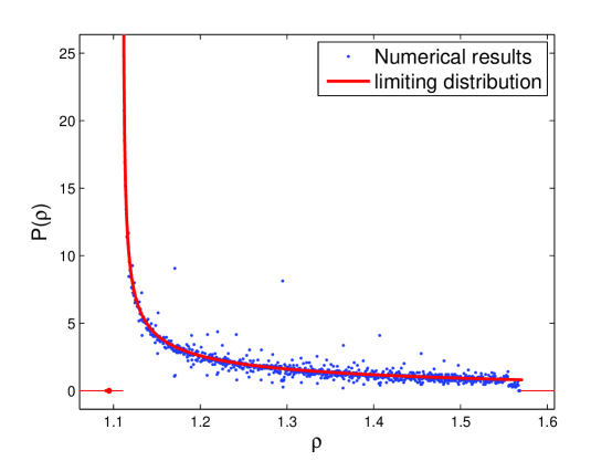
Figure 1: The limiting distribution for a rectangular billiard (13) compared to the calculated distribution for eigenfunction with $E\cdot\mathcal{A}<10^{5}$

The explicit form of $P_{rec}(\rho)$ suggests the following qualitative and quantitative conclusions:

1. The existence of a limiting distribution function (which is independent of the aspect ratio $a/b$ of the billiard) is demonstrated.

2. It is supported by the compact interval $\left[\pi/\sqrt{8},\pi/2\right]$ .

3. $P_{rec}(\rho)$ is an analytic and monotonic decreasing function in the interval where it is supported.

4. $P_{rec}(\pi/\sqrt{8}+\delta)_{{}_{\delta\rightarrow 0^{+}}}\sim\ 1/\sqrt{\delta}$ .

5. $P_{rec}(\pi/2)=8/\pi^{2}$, Hence, $P_{rec}(\rho)$ is discontinuous at both boundaries of the support.

The fact that $\rho_{mn}$ depends solely on the partition of the energy between the modes was a key element in the construction above, and plays a similar role in computing $P(\rho)$ for the other separable systems. When $\rho=\pi/\sqrt{8}$, we get from equation (2) that $E_{m}=E_{n}$, while $\rho=\pi/2$ means that the energy is concentrated completely in one degree of freedom. The concentration of probability near $\rho=\pi/\sqrt{8}$ shows that equal partition of energy is prevalent among the nodal domains.

An explicit derivation of the limiting distribution $P(\rho)$ for the family of simple surfaces of revolution (following Bleher [23]) can be found in A, in addition to a separate derivation for the disc billiard. In both cases it is proven that:

$$P_{sep}(\rho)=P_{rec}(\rho)\cdot T(\rho)$$ (14)

Where $P_{rec}$ is given by (13), and $T(\rho)$ is a finite, positive and smooth function of $\rho$. Therefore the features which characterize $P_{rec}(\rho)$ dominate $P_{sep}(\rho)$ for all the systems considered; Thus $P_{sep}(\rho)$ is supported on the same interval and demonstrates the same type of discontinuities at its boundaries.
Following the striking similarity of the distributions for all of the investigated manifolds, we suggest that properties (i)-(v) of $P_{rec}(\rho)$ which were derived for the rectangular billiard, are universal features of $P_{sep}(\rho)$ for all two-dimensional separable surfaces. We support this assumption by a heuristic model which is presented in A.

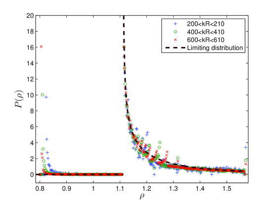
Figure 2: Semi-Classical approximation of the limiting distribution for the disc billiard compared with numerical results for 3 different energy intervals: $200<kR<210$, $400<kR<410$ and $600<kR<610$ where $k\equiv\sqrt{E}$

Numerical simulations for the rectangle and the disc billiards for several energy intervals show good agreement with the analytic derivation (see figures 1,2). For numerically obtained results at finite energies, two kinds of deviations from the limiting distributions can be observed:

1. Fluctuations along the entire range of $\rho$ (for the disc) or discrete jumps (for the rectangle) in the value of $P(\rho)$, which vanish in the limiting distribution due to the convergence of the corrections to the semi-classical approximations (i.e. turning sums over quantum numbers into integrals and the neglect of terms of order $E^{-\frac{1}{2}}$).

2. Cusps near $\rho=\frac{\pi}{4}$ and $\rho=\frac{\pi}{2}$ for the disc: the origin for the appearance of these features is due to nodal domains with exceptional geometry - the inner domains of all wavefunctions (which are asymptotically triangles) for the former, the domains of $\Psi_{n,0}$ (which are ring shaped) for the latter.

It is verified (analytically and numerically) that these differences converge to zero as $E^{-\frac{1}{2}}$, or faster.

3 The limiting distribution of the area-to-perimeter ratio for the random-wave ensemble and chaotic domains

While for chaotic wavefunctions there is no known analytic expression for the nodal lines, we will use known results about the morphology of the nodal set in order to propose some physical arguments for the expected distribution. The explanations we propose are all in agreement with numerical simulations - a detailed information about the numerical techniques and the reliability of the results can be found in appendix B.
A frequently used model for eigenfunctions in a chaotic billiard is that of the Gaussian random-wave ensemble. This is based on a conjecture by Berry [5] that eigenfunctions of a chaotic billiard in the limit of high energies have the same statistical properties as the Gaussian random-wave ensemble.
A solution $\psi$ for the Helmholtz equation (1) with a given energy $E=k^{2}$ on a given domain, can be written as a superposition of functions $\{\psi_{l}({\mathbf{r}})\}_{l=-\infty}^{\infty}$ which span a complete basis, for example:

$$\psi({\mathbf{r}})=\sum_{l=-\infty}^{\infty}a_{l}J_{l}(kr)e^{il\phi}$$ (15)

Since the solutions of (1) are real, we are restricted (for this choice of basis) by $a_{-l}=(-1)^{l}a_{l}^{*}$. According to Berry’s conjecture, expanding the eigenfunctions of chaotic billiards (in the high energy limit) in terms of (15), the coefficients $a_{l}$ distribute for $l\geq 0$ as independent gaussian random variables with

$$\langle a_{l}a_{l^{\prime}}^{*}\rangle=\delta_{l,l^{\prime}}$$ (16)

and therefore can be modeled statistically by this ensemble of independently distributed Gaussian random-waves.

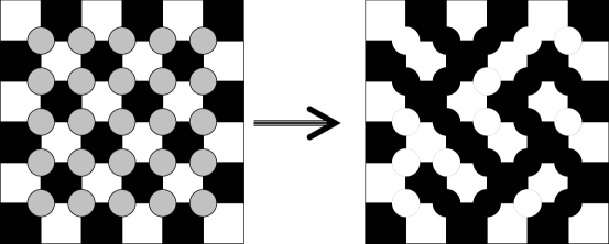
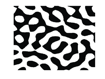
Figure 3: Above - a realization of the bond-percolation model by Bogomolny and Schmit. The dark sites are positive, and the bright are negative; at each junction there is a saddle which can be positive or negative with equal probability, connecting by that two of its neighbors to the same cluster. Below - a typical realization of the nodal structure of a random-wave on the wavelength scale.

As suggested by Bogomolny and Schmit [11], the nodal domains of a random wave are shaped as critical percolation clusters (see Figure 3), where each site is of an average area

$$\mathcal{A}_{s}=\frac{2\pi^{2}}{k^{2}}$$ (17)

where, as before, $k\equiv\sqrt{E}$. The area (or alternatively, the number of sites) of the nodal domains (see e.g. [24]) distributes (asymptotically) as a power law:

$$p(n)\propto n^{-\tau}$$ (18)

Where (for 2d percolation): $\tau=187/91$. For bond-percolation model over a lattice (as illustrated in fig. 3), the area of a cluster which spreads on $n$ sites is $(a_{1}+a_{2})n-a_{2}$ where $a_{1}$ is the area of a single site and $a_{2}$ is the area of the connection between two sites; the average perimeter is $(l_{1}+l_{2})n-l_{2}$ where $l_{1},l_{2}$ are the average contributions to the perimeter of a site and a connection (Since a cluster may contain loops which affect its perimeter, we must speak about average). The average area-to-perimeter ratio can be written as

$$\frac{A}{L}=\mathcal{C}_{1}\left(1-\frac{\mathcal{C}_{2}}{n+\mathcal{C}_{3}}\right)$$ (19)

where $\mathcal{C}_{1},\mathcal{C}_{2},\mathcal{C}_{3}>0$. This relation can be used as a guideline to the desired distribution of $\rho$.
Indeed, as was confirmed numerically, the distribution $P(\rho)$ for nodal domains follows (19) in several aspects. We have examined the restricted distribution for nodal domains with a given number of sites - we define $P^{(n)}(\rho)$ to be the distribution for nodal domains with area

$$(n-\frac{1}{2})\mathcal{A}_{s}<\mathcal{A}^{(n)}\leq(n+\frac{1}{2})\mathcal{A}_{s}$$ (20)

We found out that $P^{(n)}(\rho)$ is roughly symmetric about a mean value: $\langle\rho_{n}\rangle$. As in (19), $\langle\rho_{n}\rangle$ is increasing with $n$, and converging to a limiting value: $\rho_{\infty}$. Since the percolation model is assumed to provide an exact description of the system in the high-energy limit, we expect (19) to serve as a good approximation for large domains (see fig. 5).
The value of $\rho_{\infty}$ is a direct result of a theorem by Cauchy for the average chord length of a domain:

$$\langle\sigma\rangle=\frac{\pi\cdot A}{L}$$ (21)

Where $\sigma$ is the chord length. The original theorem (which was stated for convex domains) is extended in [25], to include nonconvex and multiply connected domains.
For nodal domains of infinite size, the statistics of the average chord length should follow that of the entire nodal set. That in turn is known to be [5, 26]: $\langle\sigma_{RW}\rangle=\sqrt{2}\pi/k$, therefore:

$$\rho_{\infty}=\frac{\langle\sigma_{RW}\rangle\cdot k}{\pi}=\sqrt{2}$$ (22)

The value of $\langle\rho_{1}\rangle$ can also be estimated: as shown in [10], the single cell nodal domains are mild deformations of a circle of radius $r=j_{0}/k$ (where $j_{0}\approx 2.405$ is the first zero of $J_{0}$). Therefore:

$$\langle\rho_{1}\rangle=\frac{\pi r^{2}k}{2\pi r}=\frac{j_{0}}{2}$$ (23)

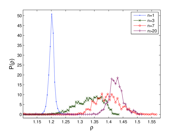
Figure 4: The distribution function $P^{(n)}(\rho)$ is plotted for several values of $n$. The mean value is increasing with $n$, while the variance decreases (except for $n=1$) as suggested by the heuristic model.

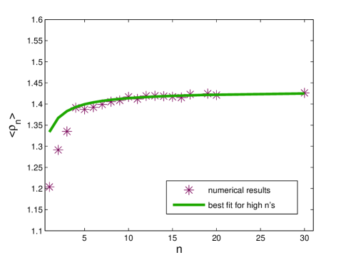
Figure 5: The measured value of $\langle\rho_{n}\rangle$ compared to the best numerical fitting (for high values of $n$) to (19): $\langle\rho_{n}\rangle=\sqrt{2}(n+0.805)/(n+0.936)$.

In order to study the impact of the deformations on the value of $\langle\rho_{1}\rangle$, we have calculated $\rho$ for a variety of domains, like ellipses, rounded shapes with corners (a quarter of a circle or a stadium etc.) and others. The results show that stretching of the nodal domain (e.g. increasing the eccentricity of an ellipse) increases $\rho$, while turning it “polygonal“ (i.e. having points on the nodal line with very high curvature) reduces $\rho$.
Derivation of  $\langle\rho_{n}\rangle$  for other values of $n$ seems to be more complicated. However, fitting between the numerical results for high $n$ values and (19) equips us with the empirical result (which is valid for $n\gg 1$):

$$\langle\rho_{n}\rangle\approx\sqrt{2}\cdot\frac{n+0.805}{n+0.936}$$ (24)

Another interesting feature is the width of the distribution around $\langle\rho_{n}\rangle$. Equation (21) implies that the variance is proportional to the variance in the average chord length between different nodal domains of the (approximately) same area. Therefore, the variance is expected to be smaller for larger domains, which follows the statistics of the entire nodal network to a larger extent. The only exception is the variance for single site domains, which as was mentioned [10], have strong limitations on their shape, and therefore a relatively small variation in the average chord length.
The bounds (6) on $\rho$ should not hold in general for the nodal domains of (15); however, the numerical bounds seem to agree with (6) for all of the measured nodal domains, including multiply connected domains, suggesting that (6) is valid for the nodal domains of the ensemble with probability 1.

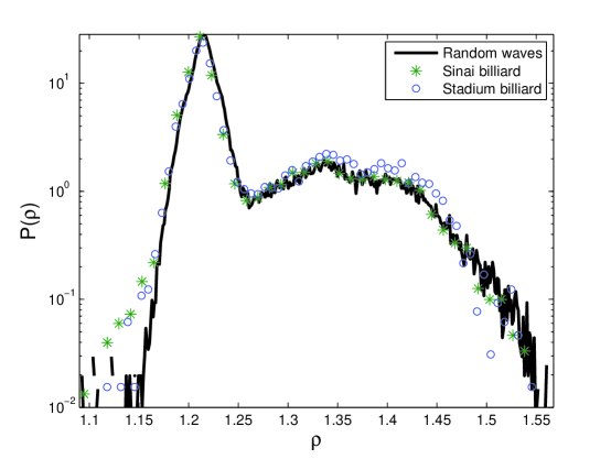
Figure 6: A comparison between the distribution function $P(\rho)$ calculated for the random-wave ensemble and for inner domains of a Sinai and stadium billiards.

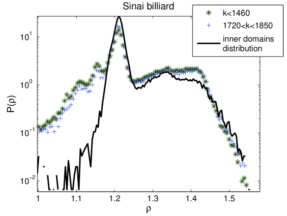
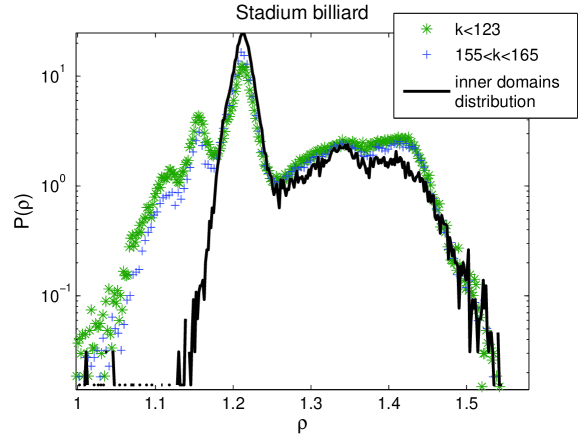
Figure 7: The distribution function $P(\rho)$ for a Sinai and stadium billiards. We compare the distribution for relatively low energy intervals (asterisks), higher intervals (crosses) and inner domains only (solid line). The distribution function indeed (slowly) converges to the distribution of inner domains (the peaks at $\pi/\sqrt{8}$ and $\sqrt{2}$ are lowered, the one at $j_{0}/2$ is elevated), which is similar to the distribution for the random-wave ensemble (see fig. 11)

The distribution of $\rho$ for all of the nodal domains is given by:

$$P(\rho)=\sum_{n=1}^{\infty}p(n)P^{(n)}(\rho)$$ (25)

where $p(n)$ is given asymptotically by (18).
Fig. 6 shows the calculated distribution for 3 different systems - A random-wave ensemble, the inner domains of a Sinai billiard and those of a stadium billiard. Comparing the functions, we find additional strengthening to Berry’s conjecture. There are boundary effects of chaotic billiards - e.g. a peak in the distribution $P(\rho)$ near $\pi/\sqrt{8}$ and $\sqrt{2}$, and a lower probability for $\rho\sim j_{0}/2$, however they vanish in the semi-classical limit (see fig. 7). In our study it was easy to put those effects aside - if we consider only inner nodal domains for the chaotic billiards (as in fig. 6), we observe no prominent differences between the distributions.

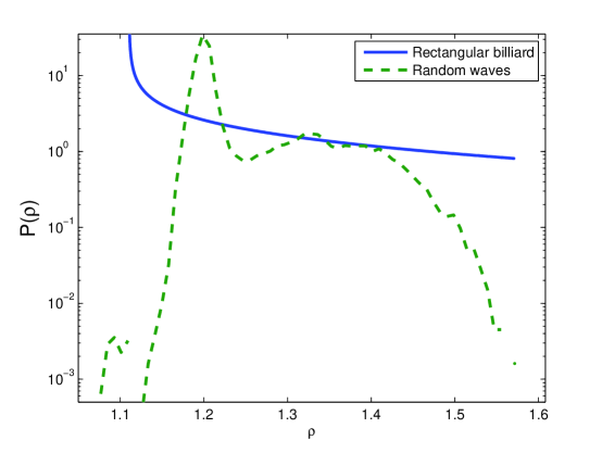
Figure 8: A comparison between the limiting distribution (13) derived for the rectangle billiard and the random-wave ensemble.

4 Conclusions

The main results of this work can be summarized as follows:

1. The distribution function $P(\rho)$ of the area-to-perimeter ratio $\rho$, distinguishes between billiards with separable or chaotic classical limit (see fig. 8).

2. The distribution (14) for the examined separable billiards has some universal features, such as a common support and a square-root divergence at the lower support. In all studied cases the distribution is a mild deformation of the distribution that we found for a rectangle.

3. In accordance with the random-wave conjecture, we find numerically that chaotic billiards (stadium and Sinai) have a universal limiting distribution $P(\rho)$, and it converges to the distribution found for the random-wave ensemble. By considering only the inner nodal domains for billiards, the agreement can be shown also for finite energies.

4. The numerical results suggest that for nodal domains of a random wave or of eigenfunctions of chaotic billiards, the area-to-perimeter ratio is bounded by (6), i.e. $\pi/4\leq\rho_{rw}\leq\pi/2$, including nonconvex and multiply connected nodal domains (for which these bounds have not been proven), with probability one.

5. We examined the percolation model for the nodal set of random waves from the perspective of the area-to-perimeter ratio. It is shown that on the wavelength scale the geometry of the nodal domains can only be poorly characterized by percolation arguments. However, for large domains the geometry can be described by heuristic expressions like (19), which are consistent with percolation theory.

Appendix A Derivation of the area-to-perimeter distribution for some separable surfaces

In this appendix we suggest a heuristic model for the universal features of the limiting distributions of the area-to-perimeter ratio for two-dimensional separable domains. The model is supported by an explicit derivation of the limiting distribution for the disc billiard and for simple surfaces of revolution.

A.1 Universal features of the distribution

We begin by considering the classical geodesic flow in a two-dimensional compact domain (e.g. a billiard). For a separable domain, a trajectory can be specified by its action-variables:

$$m=\oint p_{1}dq_{1}\quad,\quad n=\oint p_{2}dq_{2}$$ (26)

where $q_{1},q_{2}$ are the (separable) coordinates, $p_{1},p_{2}$ are the conjugated momenta and the integration is over one period of the specified coordinate. At every point along the trajectory, the energy $E_{mn}=\frac{1}{2}\left|{\mathbf{\dot{q}}}\right|^{2}$ can be expressed as $E_{mn}=E_{m}+E_{n}$, where:

$$E_{m}\equiv\frac{1}{2}\left|{\mathbf{\dot{q}}}\cdot\hat{{\mathbf{q}}}_{1}\right|^{2}\quad,\quad E_{n}\equiv\frac{1}{2}\left|{\mathbf{\dot{q}}}\cdot\hat{{\mathbf{q}}}_{2}\right|^{2}$$ (27)

where $\hat{{\mathbf{q}}}_{1},\hat{{\mathbf{q}}}_{2}$ are the local unit vectors - if we consider circular domain for example, then $\hat{{\mathbf{q}}_{1}}\equiv\hat{{\mathbf{r}}}=(\cos\theta,\sin\theta),\hat{{\mathbf{q}}_{2}}\equiv\hat{{\mathbf{\theta}}}=(-\sin\theta,\cos\theta)$. In general $E_{m},E_{n}$ are not constants of motion. The only exceptions are the trajectories in a rectangular billiard.

From a quantum point of view, the eigenstates of Schrödinger equation (1) for a separable domain, can be written as $\psi_{mn}=\psi_{m}(q_{1})\psi_{n}(q_{2})$, while the Laplace-Beltrami operator can be written as: $\Delta=\Delta_{m}+\Delta_{n}$, where $\Delta_{m}\psi_{n}=\Delta_{n}\psi_{m}=0$. This allow us to define the quantum analogue to (27):

$$E_{m}(q_{1},q_{2})=-\frac{\Delta_{m}\psi(q_{1},q_{2})}{\psi(q_{1},q_{2})}\quad,\quad E_{n}(q_{1},q_{2})=-\frac{\Delta_{n}\psi(q_{1},q_{2})}{\psi(q_{1},q_{2})}$$ (28)

In the semi-classical limit, the spectrum of a separable domain is given by $\{E_{mn}|{m,n\in\mathbb{N}}\}$, where $E_{mn}$ is the energy of the classical trajectory specified by the action-variables $m\hbar,n\hbar$ (as emerging from Bohr-Sommerfeld quantization). In addition the semi-classical value of (28) converges to the classical value (27) for every point in the domain.

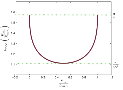
Figure 9: The value of $\rho$ as a function of the partition of energy between the two degrees of freedom, for the rectangular billiard.

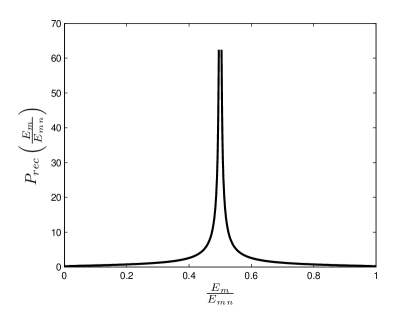
Figure 10: The limiting distribution of the partition of energy between the two degrees of freedom for a rectangular billiard.

In section 2, the value of the area-to-perimeter ratio for a given realization $\psi_{mn}$ for the rectangular billiard, was derived to be

$$\rho_{mn}=\frac{\pi}{2}\left({\sqrt{\frac{E_{m}}{E_{mn}}}+\sqrt{1-\frac{E_{m}}{E_{mn}}}}\right)^{-1}$$ (29)

Therefore, for a rectangular billiard, the value of the (quantum) parameter $\rho$, has also an immediate classical interpretation (see figures 9,10).
In order to generalize the limiting distribution which was derived for a rectangular domain to other separable domains, we suggest the following heuristic model:

• In the high energy limit, (almost all of) the nodal domains of a separable domain are converging to rectangles, and the wave function in the close neighborhood of a nodal domain is converging to (7). Therefore (in the limit) equation (29) should hold. However, since for general separable domains $\psi_{mn}({\mathbf{r}})$ is not an eigenfunction of the operators $\Delta_{m},\Delta_{n}$, the value of $\rho_{mn}^{(j)}$ for a given realization $\psi_{mn}$ will depend on the interrogated nodal domain $\omega_{j}$ .

• In the continuum limit, the limiting distribution is of the form:

  $$P(\rho)=\frac{1}{N_{I}}\int_{I}g(m,n)\int_{\mathcal{M}}\delta\left(\rho-\rho_{mn}^{(j)}\right)$$ (30)

  where the first integral is over the energy interval, and the second is over the domain. The function $g(m,n)$ is the quotient of the appropriate Jacobian and $\nu_{mn}$. Since in the vicinity of $\rho=\pi/\sqrt{8}$ two solutions for (2) coalesce, we expect the square root singularity at $P(\rho\rightarrow\pi/\sqrt{8}^{+})$ to be a universal feature.

• In addition, since $\rho(E_{m}/E_{mn})$ is convex (see equation 29 and figure 9), the distribution function should be monotonically decreasing.

This supports the assumption that the properties (i)-(iv) for $\rho_{rec}$ and $P_{rec}(\rho)$, which were derived in section 2 for the rectangle, are universal features of $P(\rho)$ for all two dimensional separable surfaces. Moreover, this model suggest - at least for separable domains - that a geometric feature of the nodal pattern, i.e. the area-to-perimeter ratio of a given domain, can be deduced directly from the underlying classical dynamics.

The suggested model is supported by an explicit derivation of the limiting area-to-perimeter distribution for several separable domains. In these calculations we approximate eigenfunctions and eigenvalues by the WKB method. In addition, we approximate sums over quantum numbers (see eq. 3) by integrals and neglect terms of order $E^{-\frac{1}{2}}$. The error resulting from these approximations is of the order of $E^{-\frac{1}{2}}$ and therefore converge to zero in the limit.
The theme of the derivations is similar. The Hamiltonian $\mathcal{H}$ for these systems is homogeneous i.e.:

$$\mathcal{H}(\lambda m,\lambda n)=\lambda^{2}\mathcal{H}(m,n)$$ (31)

This implies that the energy of the state $\psi_{mn}$ can be expressed as:

$$\mathcal{H}(m,n)=m^{2}\mathcal{H}\left(1,\frac{n}{m}\right)=m^{2}\cdot h\left(\frac{n}{m}\right)$$ (32)

Therefore, integration over the quantum number $m$ becomes trivial. We will also use the first term in the Weyl series: $\sharp\{j:E_{j}<E\}=4\pi E/\mathcal{A}+O(\sqrt{E})$ in order to estimate $N_{I}$.

A.2 The disc billiard

Equation (1) can be written in polar coordinates as

$$\left(\frac{\partial^{2}}{\partial r^{2}}+\frac{1}{r}\frac{\partial}{\partial r}+\frac{1}{r^{2}}\frac{\partial^{2}}{\partial\theta^{2}}+E\right)\psi(r,\theta)=0$$ (33)

For the disc billiard the boundary condition are: $\psi|_{r=1}=0$. The eigenfunction and eigenvalues of (33) are:

$$\psi_{mn}(r,\theta)=\cos(m\theta+\varphi)J_{m}(j_{mn}r)\quad,\quad E_{mn}={j_{mn}}^{2}$$ (34)

where $\varphi$ is an arbitrary phase and $j_{mn}$ is the $n$th zero of $J_{m}(r)$. The nodal domains of $\psi_{mn}$ will be $2m$ replicas (or one for $m=0$) of a slice containing $n$ domains ; we will enumerate them as $\{\omega_{mn}^{(i)}\}_{i=1\dots n}$, where $\omega_{mn}^{(1)}$ is the most inner domain. The area and perimeter of $\omega_{mn}^{(i)}$ are:

$$\mathcal{A}_{mn}^{(i)}=\frac{\pi}{2m}\frac{j_{mi}^{2}-j_{m,i-1}^{2}}{j_{mn}^{2}}$$ (35)

$$L_{mn}^{(i)}=\frac{\pi}{m}\frac{j_{mi}+j_{m,i-1}}{j_{mn}}+2\frac{j_{mi}-j_{m,i-1}}{j_{mn}}$$

An implicit semi-classical expression for $j_{mn}$ can be deduced by applying the WKB approximation to (33):

$$n=\int_{\frac{m}{j_{{}_{mn}}}}^{1}\sqrt{j_{mn}^{2}-{{m^{2}}\over{r^{2}}}}dr\Rightarrow$$ (36)

$$\quad\quad\quad\quad\quad j_{mn}=\pi A_{mn}\left(n+\left({1\over 2}-C_{mn}\right)m\right)$$

where:

$$C_{mn}={1\over\pi}\arctan\left(\sqrt{{m^{2}}\over{j_{mn}^{2}-m^{2}}}\right)$$ (37)

$$A_{mn}=\sqrt{1+{{m^{2}}\over{\pi^{2}\left(n+\left({1\over 2}-C_{mn}\right)m\right)^{2}}}}$$

Setting $z={n\over m},z^{\prime}={i\over m}$, and substituting (36) into (37) we get:

$$z={{\cot(\pi C_{mn})}\over\pi}+C_{mn}-{1\over 2}$$ (38)

which implies that $C_{mn}$ depends on $z$ solely. Since $A_{mn}$ varies with $n$ as $E^{-\frac{1}{2}}$, we can approximate: $A_{mn}\approx A_{m,n-1}$. Expressing $\rho_{mn}^{(i)}$ in terms of (36,37) yields:

$$\rho_{mn}^{(i)}=\frac{\frac{\pi\left({j_{mi}}^{2}-{j_{m,i-1}}^{2}\right)}{2m}}{\frac{\pi}{m}\left(j_{mi}+j_{m,i-1}\right)+2\left(j_{mi}-j_{m,i-1}\right)}$$ (39)

$$\quad\quad\quad\quad\quad\quad\quad\quad\quad\quad={\pi\over 2}\sqrt{1\over{1+\sin\left(2\pi C(z^{\prime})\right)}}$$

Bearing in mind that for a point ${\mathbf{r}}\in\omega_{mn}^{(i)}$:

$$E_{m}({\mathbf{r}})=\frac{1}{r^{2}\psi}\frac{\partial^{2}\psi}{\partial\theta^{2}}=\frac{m^{2}\cdot j_{mn}^{2}}{j_{mi}^{2}}(1+O(n^{-1}))$$ (40)

It can be shown that equation (39) is equivalent to (29).
Integrating (3) over the variables $m,C\equiv C(z),C^{\prime}\equiv C^{\prime}(z^{\prime})$, we get:

$$P_{I}(\rho)=-{8\over{\epsilon g}}\int_{I}dmdC{1\over z}{{dz}\over{dC}}\int_{C}^{1\over 2}\delta\left(\rho-{\pi\over 2}\sqrt{1\over{1+2\sin(2\pi C^{\prime})}}\right)dC^{\prime}$$ (41)

Performing the integration we get the limiting distribution:

$$P(\rho)= {4\over{\rho\sqrt{8\rho^{2}-\pi^{2}}}}\times$$

$$\frac{\pi}{2}\left({{4\rho^{2}+\pi\sqrt{8\rho^{2}-\pi^{2}}}\over{4\rho^{2}-\pi\sqrt{8\rho^{2}-\pi^{2}}}}\right.\int_{0}^{\gamma_{1}(\rho)}{{\sin(2\pi C)}\over{1+(C-{1\over 2})\pi\tan(\pi C)}}dC$$

$$+\left.{{4\rho^{2}-\pi\sqrt{8\rho^{2}-\pi^{2}}}\over{4\rho^{2}+\pi\sqrt{8\rho^{2}-\pi^{2}}}}\int_{0}^{\gamma_{2}(\rho)}{{\sin(2\pi C)}\over{1+(C-{1\over 2})\pi\tan(\pi C)}}dC\right)$$

where:

$$\gamma_{1}(\rho)={1\over{2\pi}}\arcsin\left({{\pi^{2}-4\rho^{2}}\over{4\rho^{2}}}\right)\quad;\quad\gamma_{2}(\rho)={1\over 2}-\gamma_{1}(\rho)$$ (43)

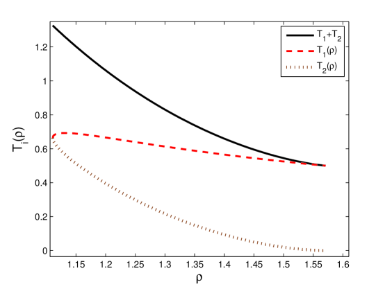
Figure 11: A realization of the functions: $T_{i}(\rho)=c_{i}(\rho)\int_{x_{i}(\rho)}{f(x)dx}$ for the disc. $T=T_{1}+T_{2}$ is monotonic, finite and positive.

A.3 Surfaces of revolution

The investigated surface of revolution $\mathcal{M}$ is generated by a rotation of the analytic profile curve $f(x)$ (where $x\in[-1,1]$) around the $x$ axis. We restrict $f(x)$ by: $f(x)_{x\rightarrow\pm 1}=a_{\pm}\sqrt{1\mp x}$, which ensures smoothness at the poles of the surface. In addition, we request that $f^{\prime\prime}(x)<0$, so $f(x)$ has a single maximum: $f_{max}\equiv f(x_{max})$.
The Lagrangian of the surface is given by:

$$\mathcal{L}={1\over 2}\left|{ds\over dt}\right|^{2}=\frac{1}{2}\left({(1+f^{\prime}(x)^{2})\dot{x}^{2}+f(x)^{2}\dot{\theta}^{2}}\right)$$ (44)

From which the action variables can be deduced:

$$m={1\over{2\pi}}\oint p_{\theta}d\theta=f(x)^{2}\dot{\theta}$$ (45)

$$n={1\over{2\pi}}\oint p_{x}dx={1\over\pi}\int_{x_{-}}^{x_{+}}{1\over{f(x)}}\sqrt{(Ef(x)^{2}-m^{2})(1+f^{\prime}(x)^{2})}dx$$

where $x_{-}$ , $x_{+}$ are the classical turning points which satisfy: $Ef(x_{\pm})^{2}-m^{2}=0$.
As in A.2 the nodal domains will be $2m+\delta_{m0}$ copies of a slice with $n$ domains and will be denoted by $\{\omega_{mn}^{(i)}\}_{i=1}^{n}$. The homogeneity of the Hamiltonian follows directly from (45). We will follow the notations $z={n\over m},z^{\prime}={i\over m}$ to get:

$$\Rightarrow E(m,z)=m^{2}\mathcal{E}^{2}(z)$$ (46)

The WKB approximation to the eigenfunctions is

$$\psi_{mz}(x,\theta)={{\cos(m\theta+\varphi)}\over\sqrt{k}}\times$$

$$\left(\cos\left(\int_{x_{-}}^{x}kdx-{\pi\over 4}\right)+\cos\left(\int_{x}^{x_{+}}kdx-{\pi\over 4}\right)\right)$$

where

$$k={m\over{f(x)}}\sqrt{(\mathcal{E}_{z}^{2}f(x)^{2}-1)(1+f^{\prime}(x)^{2})}$$

In the limit of large $n$, the nodal points density on the curve is high. Therefore, applying the WKB approximation, successive nodal points $x_{i-1}$ , $x_{i}$ should satisfy:

$$\pi=m\int_{x_{i-1}}^{x_{i}}\sqrt{\mathcal{E}_{z}^{2}f(x)^{2}-1}{\sqrt{1+f^{\prime}(x)^{2}}\over{f(x)}}$$ (48)

$$\quad\thickapprox(x_{i}-x_{i-1})m\sqrt{\mathcal{E}_{z}^{2}f(x_{i})^{2}-1}{{\sqrt{1+f^{\prime}(x_{i})^{2}}}\over{f(x_{i})}}$$

In addition, due to the homogeneity of $\mathcal{H}$, $x_{\pm}$ depend on $z$ solely, therefore:

$$\pi i=m\int_{x_{-}}^{x_{i}}\sqrt{\mathcal{E}_{z}^{2}f(x)^{2}-1}{\sqrt{1+f^{\prime}(x)^{2}}\over{f(x)}}dx\Rightarrow$$ (49)

$$z^{\prime}=\frac{1}{\pi}\int_{x_{-}}^{x_{i}}\sqrt{\mathcal{E}_{z}^{2}f(x)^{2}-1}{\sqrt{1+f^{\prime}(x)^{2}}\over{f(x)}}dx=z^{\prime}(x_{i},z)$$

Therefore, the location of the $i^{th}$ zero will be an (implicit) function $x_{i}(z,z^{\prime})$ and will not be depended on $m$. The area and perimeter of the nodal domains are:

$$\mathcal{A}_{mn}^{(i)}=\frac{\pi}{2m}\int_{x_{i-1}}^{x_{i}}f(x)\sqrt{1+f^{\prime}(x)^{2}}dx$$ (50)

$$L_{mn}^{(i)}=\frac{\pi}{2m}(f(x_{i-1})+f(x_{i}))+\int_{x_{i-1}}^{x_{i}}\sqrt{1+f^{\prime}(x)^{2}}dx$$

Therefore

$$\rho_{m,n}^{(i)}={{\pi\int_{x_{i-1}}^{x_{i}}f(x)\sqrt{1+f^{\prime}(x)^{2}}dx\sqrt{E_{nm}}}\over{\pi(f(x_{i-1})+f(x_{i}))+2m\int_{x_{i-1}}^{x_{i}}\sqrt{1+f^{\prime}(x)^{2}}dx}}=\rho(z,z^{\prime})$$ (51)

Substituting (48) in (51) we get:

$$\rho(z,z^{\prime})={\pi\over 2}{{\mathcal{E}(z)f(x_{i})}\over{1+\sqrt{(\mathcal{E}(z)f(x_{i}))^{2}-1}}}$$ (52)

where $\mathcal{E}(z)f(x_{i})=1$ at the turning points. Since for ${\mathbf{r}}\in\omega_{mn}^{(i)}$:

$$E_{m}({\mathbf{r}})=\frac{m^{2}}{f^{2}(x)}=\frac{m^{2}}{f^{2}(x_{i})}(1+O(n^{-1}))$$ (53)

Equation (51) is equivalent to (29) as well.
Integrating (3) over $m,z,z^{\prime}$ we get:

$$P_{I}(\rho)={{4\pi}\over{g\epsilon|\mathcal{M}|}}\int_{0}^{\infty}dz\int_{\frac{\sqrt{\epsilon}}{\mathcal{E}(z)}}^{\frac{\sqrt{\epsilon}(1+g)}{\mathcal{E}(z)}}dm{m\over z}\int_{0}^{z}\delta(\rho-\rho(z^{\prime}z))dz^{\prime}$$ (54)

$$\quad\quad\quad={{2\pi}\over{|\mathcal{M}|}}\int_{0}^{\infty}{{dz}\over{z\mathcal{E}(z)}}\int_{o}^{z}\delta(\rho-\rho(z^{\prime}z))dz^{\prime}$$

Setting $\alpha_{z^{\prime}z}=\mathcal{E}(z)f(x_{i}^{\prime})$, we get that for $\rho\in[\pi/\sqrt{8},\pi/2]$ and fixed $z$, there are two allowed values of $\alpha$:

$$\alpha_{1,2}={{2\rho}\over{\pi^{2}-4\rho^{2}}}\left(\pi\pm\sqrt{8\rho^{2}-\pi^{2}}\right)$$ (55)

Since $f^{-1}(x)$ is doubly valued, there are four allowed values of $z^{\prime}$:

$$z^{\prime}_{j1}=\min\left(f^{-1}\left({{\alpha_{j}}\over{\mathcal{E}(z)}}\right)\right)\quad,\quad z^{\prime}_{j2}=\max\left(f^{-1}\left({{\alpha_{j}}\over{\mathcal{E}(z)}}\right)\right)$$ (56)

for $j=1,2$. Therefore

$$P(\rho)={{2\pi}\over{|\mathcal{M}|}}\int_{0}^{\infty}{{dz}\over{z\mathcal{E}(z)^{2}}}\sum_{i}\int_{0}^{z}{{\delta(z^{\prime}-z^{\prime}_{i})}\over{\rho_{z^{\prime}z}^{\prime}(z^{\prime})}}dz^{\prime}=$$ (57)

$$P_{rec}(\rho)\cdot\left(T_{1}(\rho)+T_{2}(\rho)\right)$$

where

$$T_{1}=\frac{2\pi^{2}\rho{{(4\rho^{2}-\pi\sqrt{8\rho^{2}-\pi^{2}})^{2}}}}{|\mathcal{M}|(\pi^{2}-4\rho^{2})^{2}(\pi-\sqrt{8\rho^{2}-\pi^{2}})}\int_{z^{\prime}_{1i}}^{\infty}\sum_{i=1,2}{{dz}\over{z\mathcal{E}(z)^{3}}}\left|{{df(x_{z^{\prime}z}^{\prime})}\over{dz^{\prime}}}\right|^{-1}$$

$$T_{2}=\frac{2\pi^{2}\rho{{(4\rho^{2}+\pi\sqrt{8\rho^{2}-\pi^{2}})^{2}}}}{|\mathcal{M}|(\pi^{2}-4\rho^{2})^{2}(\pi+\sqrt{8\rho^{2}-\pi^{2}})}\int_{z^{\prime}_{2i}}^{\infty}\sum_{i=1,2}{{dz}\over{z\mathcal{E}(z)^{3}}}\left|{{df(x_{z^{\prime}z}^{\prime})}\over{dz^{\prime}}}\right|^{-1}$$

$\mathcal{E}_{z}$ is a monotonic increasing function, therefore the integrals in (57) diverges at $z=0$. For $z>>1$ , $\mathcal{E}(z)=O(z)$, therefore the integrals converge at infinity.
For $\rho\rightarrow\pi/\sqrt{8}^{+}$, the coefficient of the integrals in (57) has a square root singularity, while the integral is converging to a finite positive value, therefore $P(\pi/\sqrt{8}+\delta)\sim 1/\sqrt{\delta}$.
For $\rho\rightarrow\pi/2-\delta$, the first coefficient in (57) is of the order of $\delta$. The lower limit of integration is defined by:

$$f_{z}(z^{\prime})={{1+\delta}\over{\mathcal{E}_{z}}}=f_{z}(0)+{\delta\over{\mathcal{E}_{z}}}\Rightarrow\frac{df(z^{\prime})}{dz^{\prime}}={\delta\over{z^{\prime}\mathcal{E}_{z}}}$$ (58)

Consequently, the first term in (57) will be of order:

$$I\sim\delta\int_{z^{\prime}}^{\infty}{{z^{\prime}F(z^{\prime})dz}\over{\delta z\mathcal{E}_{z}^{3}}}$$ (59)

The value of $z^{\prime}$ depends on the profile curve $f(x)$, however for $z^{\prime}\rightarrow 0$, $I\sim z^{\prime}\log(z^{\prime})$, while for $z^{\prime}\rightarrow\infty$, we get that $I\sim 1/z^{\prime 3}$, therefore $I$ is bounded for all possible values of $z^{\prime}$.
The value of the second term is due to contributions of nodal domains which satisfy

$$\rho_{z^{\prime}z}={\pi\over 2}-\delta\Rightarrow\mathcal{E}_{z}\thicksim{1\over{f_{z}(z^{\prime})\delta}}\Rightarrow z=\frac{n}{m}\geqq O(\frac{1}{\delta})$$ (60)

Therefore, only eigenfunctions for which $n/m\geq O(1/\delta)$ contribute to the second term, as a result, it is bounded by:

$${{\int_{I}dndm\theta(n-m\delta^{-1})}\over{\int_{I}dndm}}\cong\frac{\delta g\epsilon}{\frac{|\mathcal{M}|}{4\pi}g\epsilon}\thicksim\delta$$ (61)

therefore $P(\pi/2-\delta)$ is finite, and the universal features specified in section 2 are all fulfilled by (57).

Appendix B Numerical methods for evaluation of the perimeter length

In order to evaluate the area-to-perimeter ratios and their distribution for the random-wave ensemble and chaotic billiards, we have simulated the appropriate wavefunctions on a grid.
We have calculated the statistics for 5000 realizations of random waves, where in each realization we summed over 70 terms in (15); For chaotic billiards we have reproduced the first 2430 eigenfunctions of a Sinai Billiard and the first 2725 eigenfunctions of a stadium billiard.
The (seemingly simple) task of perimeter evaluation must be carried out carefully; it can be shown that naive methods, like perimeter’s pixels counting, produce an error which is independent of the sampling resolution. In order to avoid this error, we have approximated the nodal line as a polygon, where the vortices are calculated using a linear approximation. We have set the sampling resolution to contain 85 pixels along the average distance between two nodal lines ($\sqrt{2}\pi/k$). This resolution was proved to produce an error which is less then a percent. The measured perimeter is expected to be shorter then the real one, as we are approximating a curve by a polygon.
The accuracy of the method was tested by calculating the ratio between $L_{T}$-the total length of the nodal set, and the area. It is known that for the random-wave ensemble [9]:

$$\frac{\langle L_{T}\rangle}{A\cdot k}=\frac{1}{2\sqrt{2}}$$ (62)

The numerical values for this ratio were between:

$$\frac{0.998}{2\sqrt{2}}<{\frac{L_{T}}{A\cdot k}}^{(M)}<\frac{1.003}{2\sqrt{2}}$$ (63)

It should be noted that when we calculate the total nodal length, we have to calculate the perimeter of nodal domains at the edge of the grid. In many cases (i.e. where the edge domains are very small) the perimeter calculated for them is larger then the real value. It seems likely that the error due to this effect is of the order of the error due to polygonal approximation, therefore the two compensate each other, to yield a total error which is relatively small, of order $L_{T}\cdot 10^{-3}$.

Bibliography

Bibliography

- [1] H.-J. Stöckmann, Introduction to Quantum Chaos, (Cambridge University Press, Cambridge, UK, 1999).
- [2] F. Haake, Quantum Signatures of Chaos (2nd ed., Springer, Berlin, 2000).
- [3] G. Blum, S. Gnutzmann, and U. Smilansky, Phys. Rev. Lett. 88, 114101 (2002).
- [4] T. Guhr, A. Müller-Groeling and H.A. Weidenmüller, Phys. Rep. 299, (189).
- [5] M. V. Berry. J. Phys. A 10, 2083 (1977).
- [6] R. M. Stratt, N. C. Handy, and W. H. Miller, J. Chem. Phys. 71, 3311 (1979).
- [7] H. Donnelly and C. Fefferman, Invent. Math. 93, 161 (1988).
- [8] J. Brüning, Math. Z. 158, 15 (1978).
- [9] M. V. Berry, J. Phys. A 35, 3025 (2002).
- [10] A. G. Monastra, U. Smilansky, and S. Gnutzmann. J. Phys. A 36, 1845 (2003).
- [11] E. Bogomolny and C. Schmit, Phys. Rev. Lett. 88, 114102 (2002)
- [12] J. Keating, J. Marklof, and I.G. Williams, Phys. Rev. Lett. 97,034101 (2006).
- [13] I.G. Williams, PhD thesis (Bristol, 2006).
- [14] E. Bogomolny, R. Dubertrand, and C. Schmit, J. Phys. A 40, 381 (2007).
- [15] S. Smirnov, C. R. Acad. Sci. Paris Sér. I Math. 333, 239 (2001).
- [16] G. Foltin, S. Gnutzmann, and U. Smilansky, J. Phys. A 37 11363, 2004.
- [17] P. Freitas and P. Antunes, Exp. Math. 15, 333 (2006).
- [18] R. Courant and D. Hilbert, Methods of mathematical physics. Vol. I. (Interscience Publishers, New York, 1953).
- [19] E. Makai, in G. Szego (editor) Studies in mathematical analysis and related topics, Essays in honor of George Polya, pages 227–231 (Stanford Univ. Press, Stanford, Calif., 1962).
- [20] G. Pólya, J. Indian Math. Soc. (N.S.) 24, 413 (1960).
- [21] R. Osserman, Comment. Math. Helvetici 52, 545 (1977).
- [22] H. Aiba and T. Suzuki, Phys. Rev. E 72, 066214 (2005).
- [23] P. Bleher, Duke Math. J. 74, 45 (1994).
- [24] D. Stauffer and A. Aharony, Introduction to percolation theory (2nd ed., Taylor & Francis Ltd., London, 1994).
- [25] A. Mazzolo, B. Roesslinger, and W. Gille, J. Math. Phys. 44, 6195 (2003).
- [26] S. O. Rice. Bell Systems Tech. J. 23, 282 (1944).