Controlling pulse propagation in optical fibers through nonlinearity and dispersion management

Abstract

In case of the nonlinear Schrödinger equation with designed group velocity dispersion, variable nonlinearity and gain/loss; we analytically demonstrate the phenomenon of chirp reversal crucial for pulse reproduction. Two different scenarios are exhibited, where the pulses experience identical dispersion profiles, but show entirely different propagation behavior. Exact expressions for dynamical quasi-solitons and soliton bound-states relevant for fiber communication are also exhibited.

Nonlinear Schrödinger equation (NLSE) is known to govern the pulse dynamics in nonlinear optical fibers GPA . In recent years, the study of nonlinear fiber optics, dealing with optical solitons, has attracted considerable attention since it has an important role in the development of several technologies of the 21st century HasegawaB . NLSE with distributed coefficients such as, group velocity dispersion (GVD), distributed nonlinearity and gain/loss, is being studied extensively in order to determine the effect of various distributed parameters on the pulse profile.

In the realistic situation in a fiber, there arises non-uniformity due to variation in the lattice parameters of the fiber medium, as a result of which the distance between two neighboring atoms is not constant throughout the fiber. It may also arise due to the variation of the fiber geometry e.g., diameter fluctuation. These non-uniformities influence effects such as, loss (or gain), phase modulation, etc, which can be modeled by making corresponding parameters space dependent. From a practical point of view, tailoring of various fiber parameters may lead to effective control of the pulse. This has been one of the prime motivation of a number of authors to analyze NLSE in a distributed scenario.

Dispersion management (DM) has emerged as an important technology to control and manipulate the light pulses in optical fibers HasegawaB ; Ablowitz . Pulse compression has been demonstrated with appropriately designed GVD and nonlinearity in the presence of chirping Moores ; Kruglov ; PKP , as also through soliton effects Mollenauer . Adiabatic soliton compression, through the decrease of dispersion along the length of the fiber has been shown to provide good pulse quality Dianov . The possibility of amplification of soliton pulses using a rapidly increasing distributed amplification with scale lengths comparable to the characteristic dispersion length has been reported Lisak . It has been numerically shown that, in the case where the gain due to the nonlinearity and the linear dispersion balance each other, equilibrium solitons are formed Malomed1 . Serkin and Hasegawa have formulated the effect of varying dispersion and other parameters on the soliton dynamics and have explained the concept of amplification of soliton Serkin .

The formal structure of the Lax pair for the deformed NLSE has been studied Brustev ; SerkinPRL . In a significant result, it has been numerically shown that in an appropriately designed dispersion profile chirped pulses can be retrieved through chirp reversal at a calculated location in the fiber Kumar . The advantage of pre-chirping of the input pulse in overcoming soliton interaction and dispersive-wave generation has been noted earlier Gabitov .

In the present Letter, we demonstrate analytically the phenomenon of chirp reversal of quasi-solitons with a designed dispersion profile. Very interestingly we find two possibilities of chirp reversal for which the dispersion profiles are identical. However, they exhibit entirely different propagation behavior. In one case the motion is sinusoidal and in the other it shows pulse acceleration. The procedure to control pulse dynamics is also pointed out. Exact expressions for dynamical quasi-solitons and soliton bound-states relevant for fiber communication are exhibited.

It is worth emphasizing that, exact solutions have played crucial role in demonstrating different pulse shaping techniques. The soliton solutions of NLSE or modifications of the same has come in handy in studying these mechanisms. In the same light, finding exact solutions for general types of distributed scenarios will illustrate the subtle effects and interplay of various parameters on formation and propagation dynamics of light pulses.

We develop a methodology to obtain self-similar solitary wave solutions of generalized NLSE model with varying nonlinearity, GVD, gain/loss and a confining oscillator which can be further modulated. One or few of these parameters can be switched off depending on the situation at hand. It is shown that, this equation decouples into elliptic function equation and a Schrödinger eigenvalue problem. This allows one to analytically treat a variety of distributed scenarios, a few of which we explicate in the text. In the context of Bose-Einstein condensates the procedure to deal with variable coefficient NLSE in the absence of GVD has been carried out recently by the present authors Atre . GVD leads to a fundamentally new control parameter in the present case dealing with optical fibers. For example, a subtle interplay of GVD and nonlinearity leads to a soliton bound-state as will be seen below. The effect of GVD, alternating between normal and anomalous dispersion, on pulse profile is also discussed.

For the purpose of analytic demonstration of chirp reversal we start with a NLSE model with variable GVD, nonlinearity and loss/gain Kumar :

$$i{\partial_{z}}q(z,t)+\frac{d_{e}(z)}{2}\partial_{tt}q(z,t)+\gamma(z)|q|^{2}q(z,t)+ig(z)q(z,t)=0.$$ (1)

With $q(z,t)=a(z)u(z,t)$ and $a(z)=\exp[-\int_{0}^{z}dz^{\prime}g(z^{\prime})]$, one obtains,

$$i{\partial_{z^{\prime}}}u(z^{\prime},t)+\frac{d_{e}(z^{\prime})}{2}\partial_{tt}u(z^{\prime},t)+\tilde{\gamma}(z^{\prime})|u|^{2}u(z^{\prime},t)=0,$$ (2)

where $z^{\prime}=\int_{0}^{z}dz^{\prime\prime}a^{2}(z^{\prime\prime}).$

Keeping in mind, pre-chirping and self-similar nature of the pulse we make use of the following ansatz,

$$u(z^{\prime},t)=\sqrt{p(z^{\prime})}~{}\nu\left[p(z^{\prime})t,z^{\prime}\right]\exp\left[iC(z^{\prime})t^{2}\right],$$ (3)

where, $p$ and $C$ are real functions of $z^{\prime}$.

Defining $\tau=p(z^{\prime})t,$ for preserving space-time identity one obtains

$$i\left[\frac{\partial\nu}{\partial z^{\prime}}+K_{0}\tau\frac{\partial\nu}{\partial\tau}\right] + \frac{d_{e}p^{2}}{2}\frac{\partial^{2}\nu(z^{\prime},\tau)}{\partial\tau^{2}}+\tilde{\gamma}(z^{\prime})p|\nu|^{2}\nu(z^{\prime},\tau)$$ (4)

$$- \frac{K_{1}\tau^{2}}{2}\nu+\frac{iK_{0}\nu}{2}=0,$$

where

$$K_{0}=\frac{p_{z^{\prime}}+Cd_{e}p}{p},{\mathrm{and}}~{}K_{1}=\frac{C_{z^{\prime}}+C^{2}d_{e}}{p^{3}}.$$ (5)

We now tailor the dispersion profile with $K_{0}=0$ and $K_{1}={\mathrm{const}}$:

$$i\frac{\partial\nu}{\partial z^{\prime}}+\frac{d_{e}p^{2}}{2}\frac{\partial^{2}\nu(z^{\prime},\tau)}{\partial\tau^{2}}+\tilde{\gamma}(z^{\prime})p|\nu|^{2}\nu(z^{\prime},\tau)=\frac{K_{1}\tau^{2}}{2}\nu.$$ (6)

In order to map the above equation to one with constant anomalous dispersion we assume the constraint $d_{e}p=1$ to obtain,

$$i\frac{\partial\nu}{\partial z^{\prime\prime}}+\frac{1}{2}\frac{\partial^{2}\nu(z^{\prime\prime},\tau)}{\partial\tau^{2}}+\tilde{\gamma}(z^{\prime\prime})|\nu|^{2}\nu(z^{\prime},\tau)=\frac{K_{1}\tau^{2}}{2}\nu,$$ (7)

where $z^{\prime\prime}=\int_{0}^{z^{\prime}}p(s)ds$.

The above equation has been numerically investigated, where a chirp-reversal was observed for quasi-soliton having a profile intermediate to a Gaussian and the fundamental NLSE soliton Kumar . These are stationary solutions obeying NLSE with an additional oscillator term, which explains the above profile. The exact solutions of Eq. (7) can be obtained, following the formalism developed in Ref. Atre :

$$\nu(z^{\prime\prime},\tau)=\sqrt{A(z^{\prime\prime})}F[A(z^{\prime\prime})\{\tau-\Lambda(z^{\prime\prime})\}]e^{i\Phi(z^{\prime\prime},\tau)},$$ (8)

where

$$\Phi(z^{\prime\prime},\tau)=a_{1}(z^{\prime\prime})+b(z^{\prime\prime})\tau-\frac{1}{2}c(z^{\prime\prime})\tau^{2}.$$ (9)

Here, $a_{1}(z^{\prime\prime})=a_{1_{0}}-\frac{\lambda-1}{2}\int_{0}^{z^{\prime\prime}}A^{2}(z)dz$, $\Lambda(z^{\prime\prime})=\int_{0}^{z^{\prime\prime}}v(z)dz$, which satisfies the following equation:

$$\frac{\mathrm{d}\Lambda}{\mathrm{d}z^{\prime\prime}}+c(z^{\prime\prime})\Lambda(z^{\prime\prime})=b(z^{\prime\prime}),$$ (10)

with the general solution,

$$\Lambda(z^{\prime\prime})=\{e^{\int c(z^{\prime\prime})dz^{\prime\prime}}\}^{-1}\times\left[\int dz^{\prime\prime}\left\{b(z^{\prime\prime})e^{\int c(z^{\prime\prime})dz^{\prime\prime}}\right\}\right].$$ (11)

The parameter $c({z^{\prime\prime}})$ obeys Riccati equation:

$$c_{z^{\prime\prime}}-c^{2}(z^{\prime\prime})=K_{1},$$ (12)

which can be exactly mapped to linear Schrödinger eigenvalue problem. We also find the following consistency conditions:

$$\left.\begin{array}[]{c}{\tilde{\gamma}}(z^{\prime})={\tilde{\gamma}}_{0}A(z^{\prime})/A_{0},~{}~{}b(z^{\prime\prime})=A(z^{\prime\prime})\\ A(z^{\prime\prime})=A_{0}\exp\left\{\int_{0}^{z^{\prime\prime}}c(z)dz\right\},~{}~{}A_{0}>0.\end{array}\right\}$$ (13)

$F$ obeys elliptic function equation in new variable $T=A(z^{\prime\prime})\{\tau-\Lambda(z^{\prime\prime})\}$:

$$F^{\prime\prime}(T)-\lambda F(T)+2\kappa F^{3}(T)=0,~{}{\mathrm{where}}~{}\kappa=-\frac{\gamma_{0}}{A_{0}}.$$ (14)

The twelve Jacobian elliptic functions satisfy above equation. These functions interpolate between the trigonometric and hyperbolic functions in the limiting cases Hancock . Bright soliton solutions of the type $\nu(z^{\prime\prime},\tau)=\sqrt{A(z^{\prime\prime})}~{}\mathrm{sech}[T/T_{0}]e^{i\Phi(z^{\prime\prime},\tau)}$ exist for $\kappa>0$, where $T_{0}^{2}=-A_{0}/\gamma_{0}$ and $\lambda=1/2T_{0}^{2}$, similarly kink-type dark solitons exist for $\gamma_{0}>0$. We further note that, with normal dispersion one can obtain dark solitons for $\gamma_{0}<0$. It needs to be emphasized that, in the present approach the oscillator term leads to a dynamical chirp and modulates the pulse profile. However, the pulse retains its fundamental NLSE soliton character in the scaled variable $z^{\prime\prime}$.

Below, we examine the formation of bright quasi-soliton like excitations, exhibiting chirp reversal phenomenon. This is accomplished by appropriate tailoring of GVD and pre-chirping of the launching pulse. Combining Eq. (5) and constraint $d_{e}p=1$, yield the following expressions for the tailored dispersion and the chirping parameter,

$$C=\frac{d_{e}^{\prime}}{d_{e}^{2}},~{}~{}\mathrm{and}~{}~{}d_{e}\frac{\mathrm{d}^{2}d_{e}}{\mathrm{d}z^{\prime 2}}-\left(\frac{\mathrm{d}d_{e}}{\mathrm{d}z^{\prime}}\right)^{2}=K_{1}.$$ (15)

It is interesting to notice that the choice of the constant $K_{1}$, gives rise to two scenarios, having identical dispersion and chirp profiles, but possessing entirely different pulse velocities.

We list below some explicit examples, depicting a variety of novel control mechanism for pulse manipulation.

Soliton pulses exhibiting chirp-reversal.– Inspired from the numerical investigations of Kumar and Hasegawa Kumar , we first consider in Eq. (15), $K_{1}>0$, which is equivalent to a regular oscillator potential in Eq. (7). Dispersion profile in this case reads,

$$d_{e}(z^{\prime})=\cosh(\delta z^{\prime})+\frac{C(0)}{\delta}\sinh(\delta z^{\prime}),{\mathrm{with}}~{}\delta=\left[K_{1}+C^{2}(0)\right]^{1/2}.$$ (16)

From above dispersion profile we compute launched chirp parameter $C(z^{\prime})$ and plot it together with the dynamical chirp in Fig. 1. From Eqs. (5) and (16) it is clear that launched chirp profile changes sign at $z(z^{\prime}_{c})=(1/\delta)\tanh^{-1}[-C(0)/\delta].$

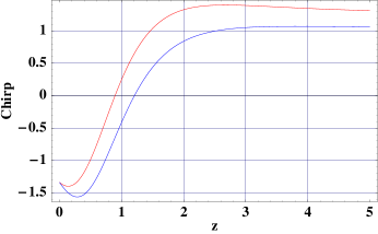
Figure 1: The figure depicting variation of chirp parameters with $z$. The red curve shows the launching chirp and the blue curve shows the same in combination with the dynamical chirp.

The expression for traveling quasi-soliton, propagating with velocity $v(z^{\prime\prime})=A_{0}\cos\left(K_{0}z^{\prime\prime}\right),$ reads

$$q(z,t) = a(z)\sqrt{p(z^{\prime})\sec(K_{1}z^{\prime\prime})}~{}\mathrm{sech}\left[\sec(K_{1}z^{\prime\prime})\{\tau-\Lambda(z^{\prime\prime})\}\right]$$ (17)

$$\times \exp\left\{{i\left[C(z^{\prime})t^{2}+\Phi(z^{\prime\prime},\tau)\right]}\right\}.$$

The presence of the dynamical chirp shifts the chirp-reversal location slightly away from $z_{c}$. Just after chirp reversal, we notice that the pulse seems to broaden, as is clearly seen in Fig. 2. Hence, the pulse needs to be retrieved at this point. With the help of a normal dispersive element such as a grating the original pulse can be recovered Belanger .

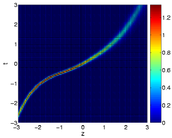
Figure 2: Pulse propagation having sinusoidal velocity profile. The plot shows broadening after chirp-reversal.

In contrast to the above example, if we consider $K_{1}<0$, we obtain $\delta=[K_{1}-C^{2}(0)]^{1/2}$, which again leads to the same dispersion profile as that of the previous example, but with the pulse velocity $v(z^{\prime\prime})=A_{0}\cosh\left(K_{0}z^{\prime\prime}\right).$ The expression for the soliton profile in this case is,

$$q(z,t) = a(z)\sqrt{p(z^{\prime})\mathrm{sech}(K_{1}z^{\prime\prime})}\mathrm{sech}\left[\mathrm{sech}(K_{1}z^{\prime\prime})\{\tau-\Lambda(z^{\prime\prime})\}\right]$$ (18)

$$\times \exp\left\{{i\left[C(z^{\prime})t^{2}+\Phi(z^{\prime\prime},\tau)\right]}\right\}.$$

It is interesting to observe that, compared with the previous case pulse broadening is significantly reduced for the same parameter values.

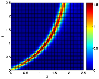
Figure 3: Soliton pulse acceleration with parameter $K_{1}<0$ implying an expulsive oscillator scenario.

Soliton bound-states.– Starting from Eq. (1) without tailoring the dispersion profile, we proceed to obtain self-similar solutions assuming the ansatz solution of the type:

$$q(z,t)=\sqrt{A(z)}F\left[A(z)\left\{\tau-\Gamma(z)\right\}\right]\exp\left\{G(z)+i\Phi(z,t)\right\}.$$ (19)

The parameters appearing in the Eq. (19) can be straightforwardly evaluated from the Eqns. (11), (12), (13) and soliton profile can be obtained from Eq. (14).

Below, we explicate some examples of spatial bound-states of solitons, arising from interplay of GVD, nonlinearity and gain/loss. Below, Fig. 4 depicts a two-soliton bound-state. This arises in a medium, where both anomalous and normal dispersion regimes are smoothly connected. In the presence of periodic gain/loss one observes modulation in the bound-state profile as is shown in Fig. 5.

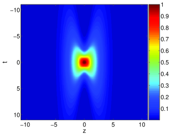
Figure 4: Soliton bound-state in a medium with two dispersion regimes.

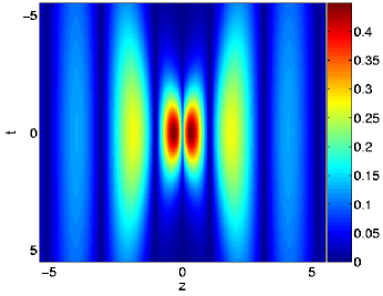
Figure 5: Multiple soliton bound-state with oscillatory gain/loss.

In conclusion, we have obtained exact soliton solutions exhibiting chirp-reversal, while retaining their original profile, crucial for pulse recovery in fiber optics. Two different soliton sectors differing in propagation behavior, but with identical dispersion profiles, are analytically exhibited. We have outlined a general formalism for obtaining self-similar solutions of nonlinear Schrödinger equation, in the presence of distributed coefficients, from which earlier scenarios follow as special cases Kruglov1 . It is shown that, this nonlinear system, involving pulse propagation with group velocity dispersion (GVD), variable nonlinearity, variable gain, exactly decouples into elliptic function equation and a Schrödinger eigenvalue problem. This opens up a number of possibilities to take into account a wide class of distributed scenarios, in close conformity with the experimentally achievable situations. This incorporates a number of special cases dealt earlier, in the context of pulse compression. We find that, apart from compression, one can achieve control over the pulse velocity, pulse profile, through interplay of group velocity dispersion, nonlinearity, gain/loss. Formation of soliton bound-states in a medium with GVD alternating between normal and anomalous dispersion, is discussed. In the presence of oscillatory gain/loss profile, we find multiple bound state structure.

We acknowledge many useful discussions with Prof. G. S. Agarwal.

References

- (1) G. P. Agrawal, Nonlinear Fiber Optics (Academic Press, Inc., San Diego, CA, 2001).
- (2) A. Hasegawa and Y. Kodama, Solitons in Optical Communications (Oxford University Press, Oxford, 1995).
- (3) M. J. Ablowitz and Z. H. Musslimani, Phys. Rev. E 67, 025601(R) (2003).
- (4) J. D. Moores, Opt. Lett. 21, 555 (1996).
- (5) V.I . Kruglov, A. C. Peacock and J. D. Harvey, Phys. Rev. Lett. 90, 113902 (2003).
- (6) T. S. Raju, P. K. Panigrahi and K. Porsezian, Phys. Rev. E 71, 026608 (2005).
- (7) L. F. Mollenauer, R. H. Stolen, J. P. Gordon, and W. J. Tomlinson, Opt. Lett. 8, 289 (1983).
- (8) E. M. Dianov, P. V. Mamyshev, A. M. Prokhorov, and S. V. Chernikov, Opt. Lett. 14, 1008 (1989).
- (9) M. L. Quiroga-Teixeiro, D. Anderson, P. A. Andrekson, A. Bernson and M. Lisak, J. Opt. Soc. Am. B 13, 687 (1996).
- (10) R. Driben and B. A. Malomed, Phys. Lett. A 301, 19 (2002).
- (11) V. N. Serkin and A. Hasegawa, IEEE J. Sel. Top. Quantum Electron. 8, 1 (2002).
- (12) S. P. Brustev, A. V. Mikhailov, and V. E. Zakharov, Theor. Math. Phys. 70, 227 (1987).
- (13) V. N. Serkin, A. Hasegawa, and T. L. Belyaeva, Phys. Rev. Lett. 92, 199401 (2004).
- (14) S. Kumar and A. Hasegawa, Opt. Lett. 22, 372 (1997).
- (15) I. Gabitov and S. K. Turitsyn, JETP. Lett. 63, 863 (1996); I. R. Gabitov and S. K. Turitsyn, Opt. Lett. 21, 327 (1996).
- (16) R. Atre, P. K. Panigrahi and G. S. Agarwal, Phys. Rev. E 73, 056611 (2006).
- (17) H. Hancock, Theory of Elliptic Functions (Dover, New York, 1958); M. Abramowitz and I. Stegun, Handbook of Mathematical Functions (NBS, US Government Printing Office, 1964).
- (18) P. A. Belanger and N. Belanger, Opt. Commun. 117, 56 (1996).
- (19) V. I. Kruglov, A. C. Peacock and J. D. Harvey, Phys. Rev. E 71, 056619 (2005); T. S. Raju, P. K. Panigrahi and K. Porsezian, Phys. Rev. E 72, 046612 (2005); V. I. Kruglov and J. D. Harvey, J. Opt. Soc. Am. B 23, 2541 (2006).