A Kinetic Theory of Coupled Oscillators

Abstract

We present an approach for the description of fluctuations that are due to finite system size induced correlations in the Kuramoto model of coupled oscillators. We construct a hierarchy for the moments of the density of oscillators that is analogous to the BBGKY hierarchy in the kinetic theory of plasmas and gases. To calculate the lowest order system size effect, we truncate this hierarchy at second order and solve the resulting closed equations for the two-oscillator correlation function around the incoherent state. We use this correlation function to compute the fluctuations of the order parameter, including the effect of transients, and compare this computation with numerical simulations.

Systems of coupled oscillators appear as models for the dynamics of a wide range of phenomena Winfree (1967); Liu et al. (1987); Golomb and Hansel (2000); Ermentrout and Rinzel (1984); Ermentrout (1991); Walker (1969); Wiesenfeld et al. (1996). The Kuramoto model is a simple and oft-studied description of coupled oscillators which, in the limit of an infinite number of oscillators, exhibits a phase transition from an incoherent state to phase locked dynamics Kuramoto (1984a, b); Kuramoto and Nishikawa (1988); Strogatz (2000). However, numerical simulations show the appearance of fluctuations that are due to finite system size effects even in the absence of any external noise. Because the system is deterministic, these fluctuations are a manifestation of multi-oscillator correlations and are expected to vanish in the infinite oscillator limit, with potentially divergent behavior near the transition Daido (1986). While there has been some effort towards an analytic treatment of the fluctuations in the Kuramoto model Kuramoto and Nishikawa (1987); Daido (1990), there is at present no systematic approach. Here, we present a statistical formalism which draws upon the kinetic theory of plasmas Ichimaru (1973); Nicholson (1992). Our methods are generalizable to any oscillator model.

The Kuramoto model describes the phase evolution of $N$ oscillators and is given by

$$\dot{\theta_{i}}=\omega_{i}+\frac{K}{N}\sum_{j=1}^{N}f(\theta_{j}-\theta_{i}),\hskip 14.45377pti=1,\ldots,N,$$ (1)

where $K$ is the coupling strength; the $\omega_{i}$ are drawn from a distribution $g(\omega)$, assumed to be symmetric and of zero mean. The coupling function $f(\theta)$ can be any function. In the original Kuramoto model $f(\theta)=\sin\theta$, which we use for our simulations.

In the $N\rightarrow\infty$ limit, Kuramoto showed Kuramoto (1984a) that as the coupling $K$ is increased from $0$, this model exhibits a phase transition described by the order parameter

$$Z=\frac{1}{N}\sum_{j=1}^{N}e^{i\theta_{j}}\equiv re^{i\psi}$$ (2)

which is a measure of the level of synchrony in the population. Kuramoto found a continuous transition from a phase of complete incoherence ($r=0$) in the population to a relative degree of coherence ($r>0$) for $K$ greater than $K_{c}=2/\pi g(0)$. However, for a finite number of oscillators, $r$ will fluctuate. Figure 1 shows $\langle r^{2}\rangle$ (where $\langle\cdot\rangle$ represents an ensemble average over frequencies and initial angles) for a numerical simulation of $N=50$ oscillators. We see that the fluctuations smooth the sharp transition from incoherence to coherence.

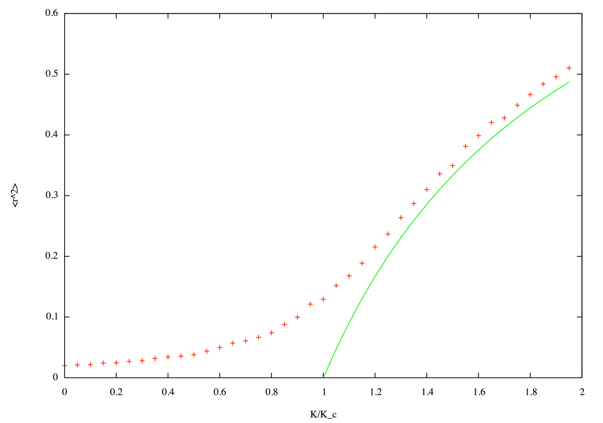
Figure 1: Phase transition in the Kuramoto model from asynchronous ($K<K_{c}$) to synchronous ($K>K_{c}$) behavior. The solid line is the mean field prediction for $r^{2}$; crosses are simulation data.

As we will show, typical with phase transitions, the correlations become enhanced near the onset of the transition (critical point). At low $K$, $\langle r^{2}\rangle\approx 1/N$, consistent with the finite size effects for the free ($K=0$) model. It reasonable to suppose that in the incoherent state all correlation effects (when $K\neq K_{c}$) are finite size effects due to the coupling, i.e. the homogeneous all-to-all connectivity forces the suppression of fluctuations as $N\rightarrow\infty$. One of our goals is to calculate $\langle r^{2}\rangle$ including the fluctuations due to finite $N$ in the incoherent state.

Mirollo and Strogatz Strogatz and Mirollo (1991) analyzed the stability of the incoherent state using a Fokker-Planck formalism. In the absence of external additive noise, their Fokker-Planck equation has the form of a continuity equation. They found that the incoherent state has a continuum of marginally stable modes, which are made stable by additive noise. In the ensuing, we will generate a series of equations analogous to the BBGKY hierarchy for which the Mirollo-Strogatz continuity equation is the truncation at first order. Our strategy is to consider an expansion using $1/N$ as a small parameter.

The complete oscillator probability density

$$n(\theta,\omega,t)=\frac{1}{N}\sum_{i=1}^{N}\delta(\theta-\theta_{i}(t))\delta(\omega-\omega_{i})$$ (3)

satisfies the continuity equation

$$\frac{\partial n}{\partial t}+\omega\frac{\partial n}{\partial\theta}=-K\frac{\partial}{\partial\theta}\int_{-\infty}^{\infty}\int_{0}^{2\pi}f(\theta^{\prime}-\theta)n(\theta^{\prime},\omega^{\prime},t)n(\theta,\omega,t)d\theta^{\prime}d\omega^{\prime}.$$ (4)

Equation (4) is analogous to the Klimontovich equation in the plasma context and is still an exact description of the microscopic dynamics. The complete oscillator distribution (3) satisfies the Klimontovich equation (4) exactly if the Kuramoto system (1) is obeyed. Solving the Klimontovich equation for the complete distribution is equivalent to solving the original system and is equally difficult. The strategy of kinetic theory is to consider the smoothed probability density functions of the oscillators by taking ensemble averages.

The one-particle probability density function (PDF) (first moment of $n(\theta,\omega,t)$) is given by

$$\rho_{1}(\theta,\omega,t)\equiv\langle n(\theta,\omega,t)\rangle$$ (5)

where brackets denote the ensemble average over initial conditions and frequencies. The density $\rho_{1}d\theta d\omega$ represents the mean fraction of oscillators within frequency range $(\omega,\omega+d\omega)$ and angle range $(\theta,\theta+d\theta)$. We note that $\int_{0}^{2\pi}\rho_{1}(\theta,\omega,t)d\theta=g(\omega)$. Henceforth, we will use the compact notation $x=(\theta,\omega)$. Taking the expectation value of Eq. (4) gives

$$\frac{\partial\rho_{1}}{\partial t}+\omega\frac{\partial\rho_{1}}{\partial\theta} + K\frac{\partial}{\partial\theta}\int_{-\infty}^{\infty}\int_{0}^{2\pi}f(\theta^{\prime}-\theta)\rho_{1}(x,t)\rho_{1}(x^{\prime},t)d\theta^{\prime}d\omega^{\prime}$$ (6)

$$= -K\frac{\partial}{\partial\theta}\int_{-\infty}^{\infty}\int_{0}^{2\pi}f(\theta^{\prime}-\theta)C(x;x^{\prime},t)d\theta^{\prime}d\omega^{\prime}$$

where

$$C(x;x^{\prime},t)=\rho_{2}(x;x^{\prime},t)-\rho_{1}(x,t)\rho_{1}(x^{\prime},t)$$ (7)

is the “connected” two oscillator correlation or moment function with

$$\langle n(x,t)n(x^{\prime},t)\rangle=\rho_{2}(x;x^{\prime},t)+\frac{1}{N}\delta(x-x^{\prime})\rho_{1}(x,t).$$ (8)

The self-fluctuation term drops out in Eq. (6) because we consider $f(0)=0$.

The RHS of (6) describes two oscillator interactions and is comparable to the collision integral from the kinetic theory of gases and plasmas. Neglecting the collision integral leads to the Vlasov equation, which amounts to a mean field approximation. The Vlasov equation and corresponding Fokker-Planck equation, which includes a diffusive term when external noise is included, has been studied for coupled oscillators previously in many contexts Strogatz and Mirollo (1991); Sakaguchi (1988); Treves (1993); Abbott and van Vreeswijk (1993); Brunel and Hansel (2006); Golomb and Hansel (2000); Cai et al. (2004); Rangan and Cai (2006). Although the Vlasov equation has the same form as Eq. (4), the two should not be confused. $\rho_{1}(x,t)$ is a smooth function representing the expectation value of the number density over initial conditions and frequencies, whereas $n(x,t)$ is an operator-valued distribution and contains all statistical information about the system.

We obtain an equation for $C(x;x^{\prime},t)$ by multiplying Eq. (4) by $n(x^{\prime},t)$ and taking the expectation value. This will result in an equation that depends on the three oscillator moment function. Continuing this process for higher moments results in the BBGKY hierarchy Ichimaru (1973); Nicholson (1992). We truncate the hierarchy at second order, expecting the correlation $C(x;x^{\prime},t)$ to be $O(1/N)$ and a general connected $n$-point function to be $O(1/N^{n-1})$ as is consistent with previous simulations Daido (1986, 1990).

Using Eq. (6) and removing terms expected to be $O(1/N^{2})$ yields

$$\{\frac{\partial}{\partial t} + \omega_{1}\frac{\partial}{\partial\theta_{1}}+\omega_{2}\frac{\partial}{\partial\theta_{2}}+K\int_{-\infty}^{\infty}\int_{0}^{2\pi}[\frac{\partial}{\partial\theta_{1}}f(\theta_{3}-\theta_{1})+\frac{\partial}{\partial\theta_{2}}f(\theta_{3}-\theta_{2})]\rho_{1}(x_{3},t)d\theta_{3}d\omega_{3}\}C(x_{1},x_{2},t)$$ (9)

$$+ K\int_{-\infty}^{\infty}\int_{0}^{2\pi}\frac{\partial}{\partial\theta_{1}}f(\theta_{3}-\theta_{1})\rho_{1}(x_{1},t)C(x_{2},x_{3},t)d\theta_{3}d\omega_{3}$$

$$+ K\int_{-\infty}^{\infty}\int_{0}^{2\pi}\frac{\partial}{\partial\theta_{2}}f(\theta_{3}-\theta_{2})\rho_{1}(x_{2},t)C(x_{3},x_{1},t)d\theta_{3}d\omega_{3}\}$$

$$= -\frac{K}{N}[\frac{\partial}{\partial\theta_{1}}f(\theta_{2}-\theta_{1})+\frac{\partial}{\partial\theta_{2}}f(\theta_{1}-\theta_{2})]\rho_{1}(x_{1},t)\rho_{1}(x_{2},t),$$

Equations (6) and (9) form a Gaussian closure of a kinetic theory describing the Kuramoto model. We use this to calculate the fluctuations about the incoherent state. We start with the ansatz Ichimaru (1973):

$$C(x_{1},x_{2},t) = \int_{-\infty}^{\infty}d\omega_{1}^{\prime}d\omega_{2}^{\prime}\int_{0}^{2\pi}d\theta_{1}^{\prime}d\theta_{2}^{\prime}\int_{t_{0}}^{t}dt\chi(x_{1}^{\prime},x_{2}^{\prime},t^{\prime})$$ (10)

$$\times P(x_{1},x_{1}^{\prime},t-t^{\prime})P(x_{2},x_{2}^{\prime},t-t^{\prime}).$$

where the initial conditions are imposed at $t_{0}$ and $t_{0}<t^{\prime}<t$. Using Eq. (10) in Eq. (9), we obtain the dynamics for the propagator $P$,

$$\{\frac{\partial}{\partial t} + \omega_{1}\frac{\partial}{\partial\theta_{1}}+K\frac{\partial}{\partial\theta_{1}}\int_{-\infty}^{\infty}\int_{0}^{2\pi}f(\theta_{2}-\theta_{1})\rho_{1}(x_{2},t)d\theta_{2}d\omega_{2}\}P(x_{1},x_{1}^{\prime},t-t^{\prime})$$ (11)

$$+ K\frac{\partial}{\partial\theta_{1}}\int_{-\infty}^{\infty}\int_{0}^{2\pi}f(\theta_{2}-\theta_{1})\rho_{1}(x_{1},t)P(x_{2},x_{1}^{\prime},t-t^{\prime})d\theta_{2}d\omega_{2}=0,$$

where

$$\chi(x_{1},x_{2},t)=-\frac{K}{N}[\frac{\partial}{\partial\theta_{1}}f(\theta_{2}-\theta_{1})+\frac{\partial}{\partial\theta_{2}}f(\theta_{1}-\theta_{2})]\rho_{1}(x_{1},t)\rho_{1}(x_{2},t)$$ (12)

and the initial condition is $P(x;x^{\prime},0)=\delta(x-x^{\prime})$.

The fluctuations in the order parameter are given by

$$\langle r^{2}\rangle\equiv\langle ZZ^{*}\rangle=\int d\omega d\omega^{\prime}d\theta d\theta^{\prime}\langle n(\omega,\theta,t)n(\omega^{\prime},\theta^{\prime},t)\rangle e^{i(\theta-\theta^{\prime})}$$ (13)

We consider fluctuations in the incoherent state and thus seek solutions to (6) and (9) such that $\rho_{1}(x,t)=\frac{1}{2\pi}g(\omega)$. From Eqs. (7) and (8), we see that a computation of the fluctuations amounts to a calculation of the connected correlation function, which is phase invariant (because $\rho_{1}$ is independent of $\theta$), so that $C(\theta_{1},\theta_{2},\omega_{1},\omega_{2},t)=C(\theta_{1}-\theta_{2},\omega_{1},\omega_{2},t)$. Hence, the collision integral in Eq. (6) is zero, making $\rho_{1}(\theta,\omega)=g(\omega)/2\pi$ an exact solution of the equations. Taking the Fourier and Laplace transforms in $\theta$ and time of Eq. (10) gives

$$C_{n}(\omega_{1},\omega_{2},s) = \frac{nK{\rm Im}[f_{n}]}{2\pi^{2}N}\int_{-\infty}^{\infty}d\omega_{1}^{\prime}d\omega_{2}^{\prime}d\tau\int_{{\cal L}_{1}}ds_{1}\int_{{\cal L}_{2}}ds_{2}g(\omega^{\prime}_{1})g(\omega^{\prime}_{2})$$

$$\times \hat{P}_{-n}(\omega_{1},\omega_{1}^{\prime},s_{1})\hat{P}_{n}(\omega_{2},\omega_{2}^{\prime},s_{2})\frac{1}{s}e^{(s_{1}+s_{2}-s)\tau},$$

where $n$ is the Fourier mode index, $s_{1,2}$ is a Laplace transform variable and $\tau=t-t^{\prime}$. By definition, the Laplace contours ${\cal L}_{1}$ and ${\cal L}_{2}$ are arranged such that they are to the right of all poles in $\hat{P}_{-n}$ and $\hat{P}_{n}$, respectively. Using Eqs. (7), (8) and (A Kinetic Theory of Coupled Oscillators) in Eq. (13) gives

$$\langle r^{2}(\tau)\rangle=4\pi^{2}\int d\omega d\omega^{\prime}C_{-1}(\omega,\omega^{\prime},\tau)+\frac{1}{N}$$ (15)

because $\langle Z\rangle=0$.

We can obtain a general expression for $\langle r^{2}\rangle$ without explicitly solving for the correlation function. From equation (11), we can derive the relation

$$\int\hat{P}_{n}(\omega,\omega^{\prime},s)d\omega=\frac{1}{(s+in\omega^{\prime})\Lambda_{n}(s)}$$ (16)

where

$$\Lambda_{n}(s)\equiv 1+inKf_{n}^{\ast}\int_{-\infty}^{\infty}\frac{g(\omega)d\omega}{s+in\omega}$$ (17)

is the analog of the dielectric response function. Using Eqs. (16) and (A Kinetic Theory of Coupled Oscillators) in Eq. (15) yields

$$\langle r^{2}(\tau)\rangle=\frac{2}{iKN\pi}\int_{{\cal C}}ds\frac{\Lambda_{1}(s-s_{0})-1}{\Lambda_{1}(s-s_{0})}{\rm Res}\left[\frac{-1}{\Lambda_{1}(s)}\right]_{s=s_{0}}\frac{1}{s}e^{s\tau}$$ (18)

where $s_{0}$ is the zero of $\Lambda_{n}(s)$. The strategy of the calculation leading to Eq. (18) is similar to the calculation of the Lenard-Balescu collision integral Ichimaru (1973); Nicholson (1992).

For the specific frequency distribution $g(\omega)=(\gamma/\pi)(1/(\omega^{2}+\gamma^{2}))$ (i.e. a Lorentz distribution), Eq. (18) evaluates to

$$\langle r^{2}(\tau)\rangle=\frac{1}{N}\frac{K_{c}}{K_{c}-K}-\frac{1}{N}\frac{K}{K_{c}-K}e^{-(K_{c}-K)\tau}$$ (19)

where $K_{c}=2\gamma$ for the Lorentz frequency distribution. $\langle r^{2}(0)\rangle=1/N$ because the initial conditions for Eqs. (6) and (9) are such that $\rho_{1}(x,0)$ is the equilibrium incoherent state and $C(x_{1},x_{2},0)=0$. For the uncoupled system $K=0$, so $\langle r^{2}\rangle=1/N$ as expected. We also see that the amplitude of the fluctuations and the transient decay time become singular at the critical point $K=K_{c}$. At criticality, we obtain the expression $\langle r^{2}(\tau)\rangle=(1/N)(1+K_{c}\tau)$. The closer $K$ is to criticality, the less this calculation should be valid. Near critical behavior requires an analysis of all orders in the $1/N$ expansion. Dynamically, the implication is that as the coupling strength nears criticality, oscillators will interact more strongly and higher order correlations will become more important. The result $\langle r^{2}(\infty)\rangle=K_{c}/[N(K_{c}-K)]$ was first derived by Daido Daido (1990) with a completely different approach. Our method facilitates a systematic expansion in $1/N$, in addition to providing an examination of the transient behavior of $\langle r^{2}(\tau)\rangle$.

We can examine the transient behavior of the correlations by solving Eq. (A Kinetic Theory of Coupled Oscillators) for the Lorentz distribution. We first solve for the propagator in Eq. (11) by taking a Fourier series expansion in $\theta$ and Laplace transform in time, to obtain

$$\hat{P}_{n}(\omega_{1},\omega_{1}^{\prime},s)=\frac{1}{s+in\omega_{1}}\frac{\delta(\omega_{1}-\omega_{1}^{\prime})}{2\pi}-\frac{inKf_{n}^{\ast}g(\omega_{1})}{2\pi(s+in\omega_{1})(s+in\omega_{1}^{\prime})\Lambda_{n}(s)}$$ (20)

where $s$ is the Laplace transform variable and $\Lambda_{n}(s)=1-(K/2)|n|/(s+|n|\gamma)$. The propagator (20) has poles along the imaginary axis corresponding to the continuous spectrum of marginally stable modes as well as those given by the discrete zeros of $\Lambda_{n}(s)$, which for $K<K_{c}=2\gamma$ are real and negative Strogatz and Mirollo (1991).

We then use Eq. (20) in Eq. (A Kinetic Theory of Coupled Oscillators) and take the inverse Laplace transform. For the $n=1$ mode, this gives

$$C_{1}(\omega,\omega^{\prime},\tau) = \frac{K}{N}\frac{1}{4\pi^{2}}g(\omega)g(\omega^{\prime})\left[\frac{(i\omega+\frac{K_{c}}{2})(-i\omega^{\prime}+\frac{K_{c}}{2})}{(i\omega+\frac{K_{c}}{2}-\frac{K}{2})(-i\omega^{\prime}+\frac{K_{c}}{2}-\frac{K}{2})}\left(\frac{e^{(i(\omega-\omega^{\prime})\tau)}}{i(\omega-\omega^{\prime})}-\frac{1}{i(\omega-\omega^{\prime})}\right)\right.$$ (21)

$$+ \frac{K}{2}\frac{(i\omega^{\prime}-\frac{K_{c}}{2})}{(\frac{K}{2}-\frac{K_{c}}{2}-i\omega)((\frac{K_{c}}{2}-\frac{K}{2})^{2}+(\omega^{\prime})^{2})}\left(e^{-(\frac{K_{c}}{2}-\frac{K}{2}+i\omega^{\prime})\tau}-1\right)$$

$$+ \frac{K}{2}\frac{(-i\omega-\frac{K_{c}}{2})}{(\frac{K}{2}-\frac{K_{c}}{2}+i\omega^{\prime})((\frac{K_{c}}{2}-\frac{K}{2})^{2}+(\omega)^{2})}\left(e^{-(\frac{K_{c}}{2}-\frac{K}{2}-i\omega)\tau}-1\right)$$

$$+ \left.\frac{K^{2}}{4(K-2\frac{K_{c}}{2})}\frac{1}{(\frac{K}{2}-\frac{K_{c}}{2}-i\omega)(\frac{K}{2}-\frac{K_{c}}{2}+i\omega^{\prime})}\left(e^{-(K_{c}-K)\tau}-1\right)\right]$$

where $\tau=t-t_{0}$. The other modes are given by $C_{-1}=C_{1}^{*}$ and $C_{n}=0$ for $n\neq\pm 1$ since $f(\theta)=\sin\theta$. The correlation function will thus have the form

$$C(\omega,\omega^{\prime},\theta-\theta^{\prime},\tau)=C_{1}e^{i(\theta-\theta^{\prime})}+C_{-1}e^{-i(\theta-\theta^{\prime})}$$ (22)

Only the last term in Eq. (21) contributes to the transient in Eq. (19). The correlation function contains modes which consist of all possible pairings of a marginal oscillating mode with the decaying mode. While the marginal modes do not decay in the correlations, they do not affect the decay of $\langle Z(\tau)\rangle$ because of a Landau damping-like dephasing effect that is described in Ref. Strogatz et al. (1992). The marginal modes also have no effect upon the transient behavior of $\langle r^{2}(\tau)\rangle$. We should expect a similar result for higher moments. At this order, the marginal modes are not rendered stable by finite size effects as they are with the addition of external additive noise Strogatz and Mirollo (1991). Should stabilization occur due to the intrinsic fluctuations, it will necessarily be a consequence of higher order effects.

We compare our analytical results to numerical simulations of the Kuramoto system. Figure 2 a) shows the asymptotic value of $\langle r^{2}\rangle$ for various values of $K$ and $N$. The analytical prediction matches extremely well for $N=500$ and reasonably well for $N=50$ and $N=100$. Only at $N=10$ are there significant deviations from the prediction. Fig. 2 b) shows the transient behavior of $\langle r^{2}\rangle$. The results match quite well below $K/K_{c}=0.8$. Numerical results for the correlation function integrated over $\omega,\omega^{\prime}$ are shown in Fig. 3. The simulation agrees well with the prediction Eq. (22) except near the critical point as expected.

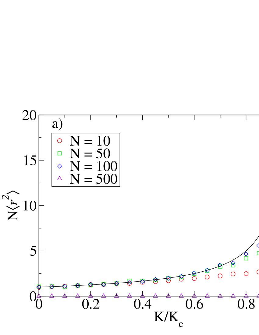
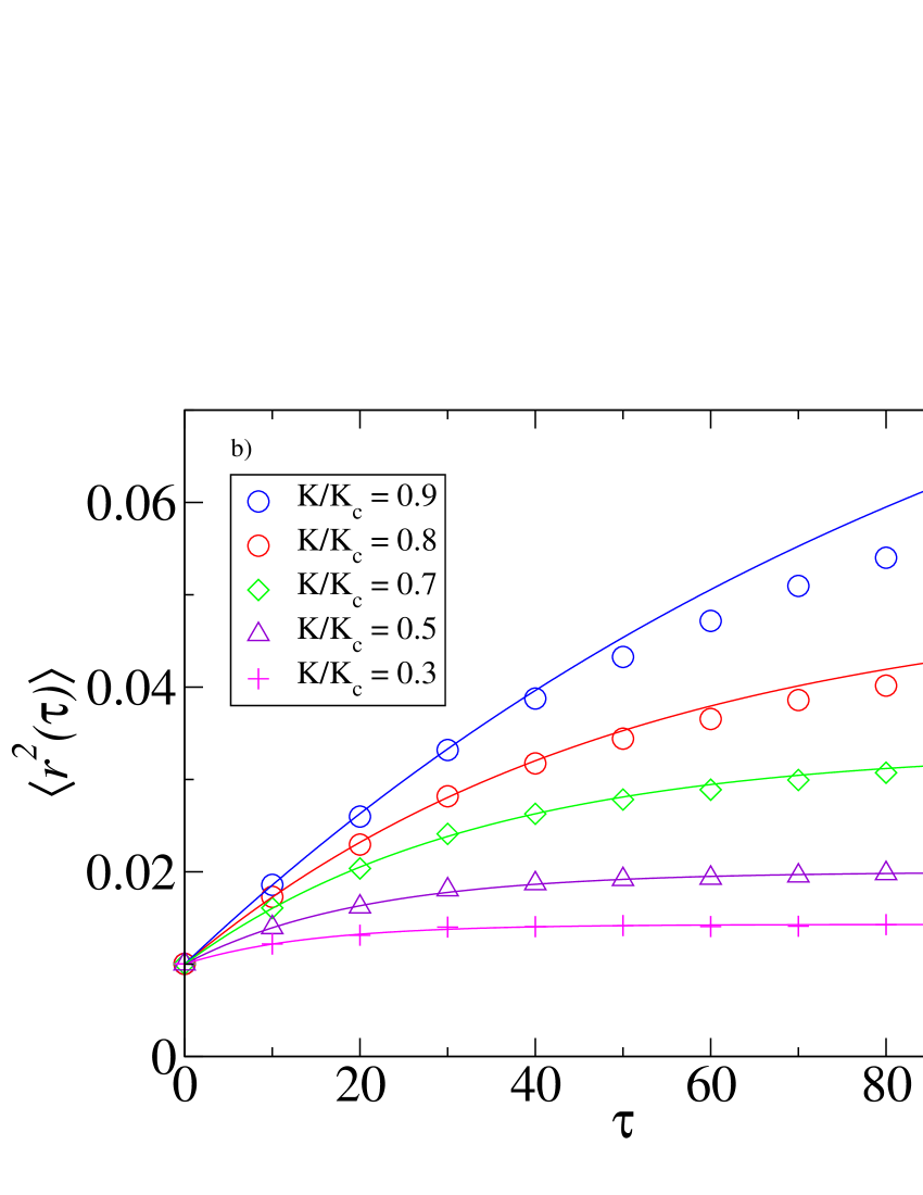
Figure 2: a) Simulated and predicted $N\langle r^{2}\rangle$ vs. $K/K_{c}$ for various values of N for large times. The data are evolved for 6 time constants at each $K$ ($\tau=1/(K_{c}-K)$) and averaged over 1000 different initial conditions and frequencies. The frequency distribution is Lorentz with $\gamma=0.05$. The simulation was performed with a time step of 0.05. The initial distribution of angles was uniform. b) Time evolution of $\langle r^{2}(\tau)\rangle$ vs. $\tau$ for various values of $K$ and for $N=100$. At each time point the values are averaged over 10,000 different initial conditions and frequencies. All other parameters as above.

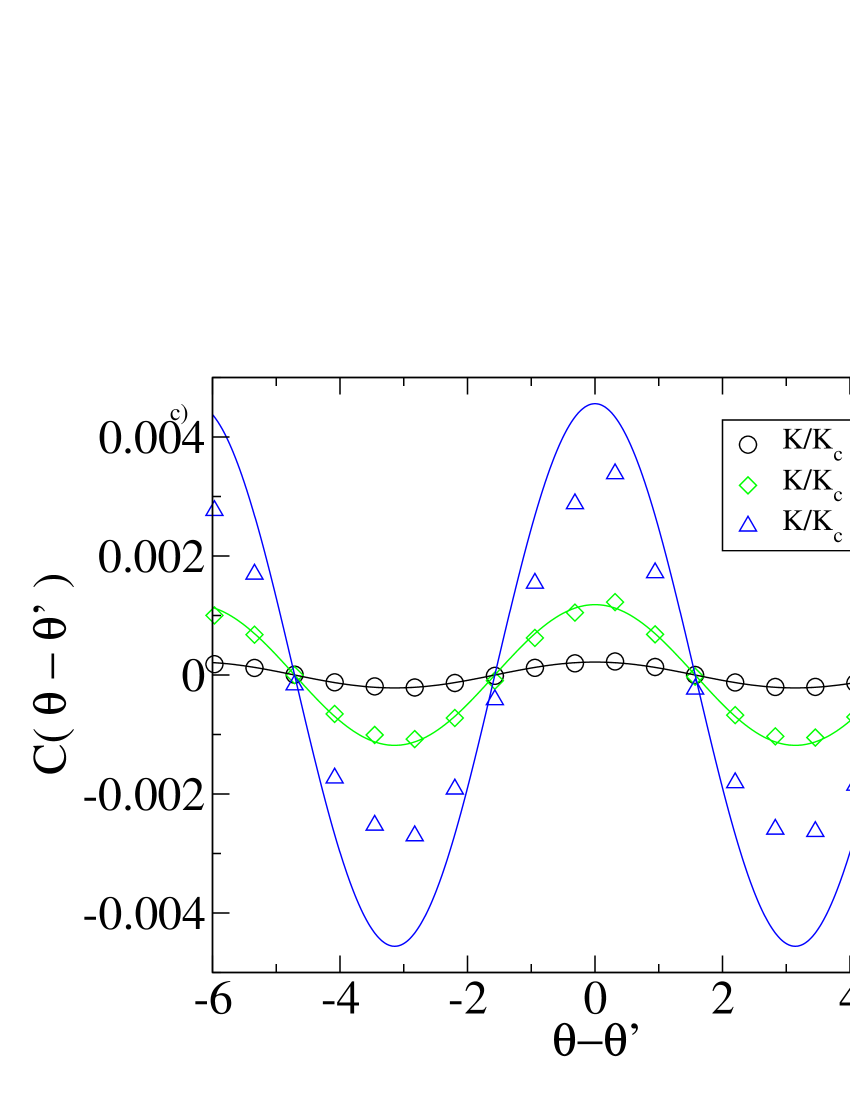
Figure 3: $C(\omega,\omega^{\prime},\theta-\theta^{\prime})$ integrated over $\omega$ and $\omega^{\prime}$ versus $\theta-\theta^{\prime}$ for $N=100$ and various values of $K$. Frequency distribution is Lorentz with $\gamma=0.05$ and the initial angle distribution is uniform. Results are averaged over 100,000 samples in a 2 dimensional histogram with 100x100 bins. The data is then averaged over angle differences and then put into a one dimensional histogram with bins of width 10. The time step for the evolution is 0.05.

Our calculation is the first presentation of a systematic approach to understanding the fluctuations due to finite size effects to an arbitrary order in $1/N$. Although we truncate at lowest order, our approach allows a truncation at any level of the moment hierarchy to produce an expansion in $1/N$. We note that Ref. Pikovsky and Ruffo (1999) found that when the oscillators are driven with Gaussian noise, $1/N$ dependence is still seen in the fluctuations of the order parameter. Additionally, our methodology could be used to study the evolution of the phase of $Z$, as in Ref. Gleeson (2006).

Some previous work  Brunel and Hansel (2006); Golomb and Hansel (2000); Treves (1993); Abbott and van Vreeswijk (1993); Crawford and Davies (1999); Pikovsky and Ruffo (1999) for both phase and pulse coupled oscillators also start with a continuity equation similar to Eq. (4) but either go directly to mean field theory, with and without an external noise source to approximate fluctuations, or assume the fluctuations are Gaussian. References Cai et al. (2004); Rangan and Cai (2006) derive a kinetic theory for a network of integrate-and-fire neurons by constructing a moment hierarchy similar to ours that is closed using the maximum entropy principle. However, this work differs from ours in that the hierarchy is built from a Boltzmann-like equation for a one-particle distribution function with stochastic inputs and hence does not capture the same correlation effects that we find by starting from a continuity equation that contains the full statistics of the system.

We feel it is important to stress that the Klimontovich continuity equation (Eq. (4)) is not an approximation. The approximation appears in the method of finding solutions. The mean field limit is equivalent to setting correlations to zero. Computing the moment hierarchy allows for an expansion which accounts for the effects of correlations. We produce a systematic method for deriving such an expansion and show explicitly in what regime higher order correlations can be ignored. We also note that the kinetic theory approach is only one avenue to understanding correlations. An alternative formulation is through a statistical field theory approach Zinn-Justin (2002), which facilitates the construction of an expansion without resorting to a moment hierarchy.

This research was supported in part by the Intramural Research Program of NIH, NIDDK.

References

- Winfree (1967) A. T. Winfree, Journal of Theoretical Biology 16, 15 (1967).
- Liu et al. (1987) C. Liu, D. Weaver, S. Strogatz, and S. Reppert, Cell 91, 855 (1987).
- Golomb and Hansel (2000) D. Golomb and D. Hansel, Neural Computation 12, 1095 (2000).
- Ermentrout and Rinzel (1984) G. B. Ermentrout and J. Rinzel, Am. J. Physiol 246, R102 (1984).
- Ermentrout (1991) G. B. Ermentrout, Journal of Mathematical Biology 29, 571 (1991).
- Walker (1969) T. J. Walker, Science 166, 891 (1969).
- Wiesenfeld et al. (1996) K. Wiesenfeld, P. Colet, and S. H. Strogatz, Physical Review Letters 76, 404 (1996).
- Kuramoto (1984a) Y. Kuramoto, Chemical Oscillations, Waves, and Turbulence (Springer-Verlag, 1984a).
- Kuramoto (1984b) Y. Kuramoto, Progress of Theoretical Physics Supplement 79, 223 (1984b).
- Kuramoto and Nishikawa (1988) Y. Kuramoto and I. Nishikawa, in Cooperative Dynamics in Complex Physical Systems, edited by H. Takayama (Springer, 1988).
- Strogatz (2000) S. H. Strogatz, Physica D 143, 1 (2000).
- Daido (1986) H. Daido, Progress of Theoretical Physics 75, 1460 (1986).
- Kuramoto and Nishikawa (1987) Y. Kuramoto and I. Nishikawa, Journal of Statistical Physics 49, 569 (1987).
- Daido (1990) H. Daido, Journal of Statistical Physics 60, 753 (1990).
- Ichimaru (1973) S. Ichimaru, Basic principles of Plasma Physics: A Statistical Approach (W.A. Benjamin Advanced Book Program, 1973).
- Nicholson (1992) D. R. Nicholson, Introduction to Plasma Theory (Krieger Publishing Company, 1992).
- Strogatz and Mirollo (1991) S. H. Strogatz and R. E. Mirollo, Journal of Statistical Physics 63, 613 (1991).
- Sakaguchi (1988) H. Sakaguchi, Progress of Theoretical Physics 79, 39 (1988).
- Treves (1993) A. Treves, Network: Computation in Neural Systems 4, 259 (1993).
- Abbott and van Vreeswijk (1993) L. F. Abbott and C. van Vreeswijk, Physical Review E 48, 1483 (1993).
- Brunel and Hansel (2006) N. Brunel and D. Hansel, Neural Computation 18, 1066 (2006).
- Cai et al. (2004) D. Cai, L. Tao, M. Shelley, and D. W. McLaughlin, Proceedings of the National Academy of Sciences 101, 7757 (2004).
- Rangan and Cai (2006) A. V. Rangan and D. Cai, Phys. Rev. Lett. 96, 178101 (2006).
- Strogatz et al. (1992) S. H. Strogatz, R. E. Mirollo, and P. C. Matthews, Physical Review Letters 68, 2730 (1992).
- Pikovsky and Ruffo (1999) A. Pikovsky and S. Ruffo, Physical Review E 59, 1633 (1999).
- Gleeson (2006) J. P. Gleeson, Europhysics Letters 73, 328 (2006).
- Crawford and Davies (1999) J. D. Crawford and K. Davies, Physica D 125, 1 (1999).
- Zinn-Justin (2002) J. Zinn-Justin, Quantum Field Theory and Critical Phenomena (Oxford Science Publications, 2002), 4th ed.