Linear response, susceptibility and resonances in chaotic toy models

Abstract

We consider simple examples illustrating some new features of the linear response theory developed by Ruelle for dissipative and chaotic systems [J. of Stat. Phys. 95 (1999) 393]. In this theory the concepts of linear response, susceptibility and resonance, which are familiar to physicists, have been revisited due to the dynamical contraction of the whole phase space onto attractors. In particular the standard framework of the “fluctuation-dissipation” theorem breaks down and new resonances can show up oustside the powerspectrum. In previous papers we proposed and used new numerical methods to demonstrate the presence of the new resonances predicted by Ruelle in a model of chaotic neural network. In this article we deal with simpler models which can be worked out analytically in order to gain more insights into the genesis of the “stable” resonances and their consequences on the linear response of the system. We consider a class of 2-dimensional time-discrete maps describing simple rotator models with a contracting radial dynamics onto the unit circle and a chaotic angular dynamics $\theta_{t+1}=2\theta_{t}(\mbox{\rm mod}\>2\pi)$. A generalisation of this system to a network of interconnected rotators is also analysed and related with our previous studies [8, 11]. These models permit us to classify the different types of resonances in the susceptibility and to discuss in particular the relation between the relaxation time of the system to equilibrium with the mixing time given by the decay of the correlation functions. Also it enables one to propose some general mechanisms responsible for the creation of stable resonances with arbitrary frequencies, widths, and dependency on the pair of perturbed/observed variables.

1 Introduction

In statistical physics, a standard idea is that the linear response of a system can be computed in terms of correlation functions of this system at equilibrium. This is the cornerstone of important results like the fluctuation-dissipation theorem [1, 2]. More recently a general theory for the linear response for hyperbolic systems has been developed by Ruelle [3, 4]. This theory shows that the picture of correlation functions is incomplete in this case. In this situation a linear response function has in general two contributions, corresponding respectively to the expanding (unstable) and the contracting (stable) directions of the hyperbolic dynamics. Although the first contribution, called in the sequel the unstable response function, can still be associated with some correlation function, this is not true for the second contribution, named the stable response function. This property transfers to the complex susceptibility, i.e. the frequency-dependent responses of the system, for which we can also distinguish between two types of resonances, namely the stable and the unstable resonances.

Computations of the linear response in specific chaotic systems have been performed by several authors [5]-[7]. For example in [5], Falcioni et al. discuss and numerically apply a simple method to calculate the (impulse) linear response function. The procedure is an averaging on perturbations of the system by means of Dirac kicks. However, as estimated by the authors, the convergence of this method is slow in the time-domain. Another study has been performed by Reick in [7], who uses a different technique, averaging the effects of time-periodic perturbations. With this method he numerically demonstrates the existence of linear response in the Lorentz system, although the latter is known to be nonhyperbolic. Neither of these previous works, however, obtain evidence of the stable resonances predicted by Ruelle. Let us remark that contrary to the present study, these papers do not consider chaotic systems with state-dependent perturbations.

In a recent work we have illustrated for the first time the prediction of Ruelle on a simple model of networks of interconnected units exhibiting chaotic dynamics [8]. Using independently the same averaging procedure as [7], we managed to compute the susceptibility $\hat{\chi}_{ij}(\omega)$ and its complex poles. (Here $\hat{\chi}_{ij}(\omega)$ denotes the complex amplitude of the average response of unit $i$ to a harmonic excitation of unit $j$ at frequency $\omega$). Our numerical method could not provide separately the unstable and the stable contributions in the susceptibility, but our results demonstrated the existence of stable poles in $\hat{\chi}_{ij}(\omega)$ by setting in evidence poles which were not in the set of poles of the correlation functions (the Ruelle-Pollicott resonances [9, 10]).

On the other hand our numerical results pointed out towards interesting features whose consequences are worth to explore further. First, stable resonances in $\hat{\chi}_{ij}$ can be specific to the pair $ij$. This property, which is not true in general for the Ruelle-Pollicott resonances, is quite useful for networks as it can be used to transmit an amplitude modulated signal between two specific units in the network [11]. Another unexpected feature is that the average relaxation time of unit $i$ to an impulse perturbation of unit $j$ (which can be predicted by Fourier transform of $\hat{\chi}_{ij}(\omega)$) can extend on a much longer time lapse than the mixing time, i.e. the decay time associated with the correlation functions.

These properties cannot be understood in the framework of the classical fluctuation-response theorem. Indeed they reflect the presence of the stable contribution of the response functions which are not correlation functions. However the stable response or the stable susceptibility are difficult to extract numerically. Therefore the goal of the present paper is to study a class of toy models for which the stable and unstable decomposition of response functions can be worked out explicitly. In particular these examples clearly show the relative contributions of correlation and non-correlation terms in the response functions, and their treatment helps to better understand the above properties revealed in networks. These simple examples are also treated numerically. This allows one to validate the numerical procedure used in [8, 11].

In the next Section we recall some elements of Ruelle’s theory which will be extensively used later on. We formally derive his general response formula by using the method of the impulse response and then introduce the definition of susceptibility as being its Fourier transform. In Section 3 we treat the basic example $\theta_{t+1}=2\theta_{t}$ (mod $2\pi$) in this framework and discuss briefly the issue of the non-invertibility of this dynamics. This elementary example serves also to describe and to test numerical methods. Section 4 concerns class of uniformly hyperbolic systems which modelise chaotic rotators in the plane. Various extensions of the simplest model are considered in the following subsections so as to discuss properties of the stable resonances. They are summarised in the Conclusions. An appendix of the paper presents a natural extension of our chaotic rotator model in higher dimensions for which some properties generalise directly.

2 A general linear response formula of Ruelle

We start by reviewing some results of the linear response theory obtained by Ruelle [3, 4]. We concentrate on the particular case of autonomous dynamical systems described by iterations of a map. Consider the following systems whose dynamics is governed by the recurrence equation:

$${\bf x}_{t+1}={\bf F}({\bf x}_{t})$$ (1)

where $t\in\mathbb{Z},\>{\bf x}\in M$, and $M$ is the phase space, e.g. a compact manifold in $\mathbb{R}^{N}$. The map is defined by a smooth function ${\bf F}({\bf x})$, not necessarily invertible, and ${\bf x}_{t}$ denotes the state of system at time $t$. We also use the notation ${\bf F}({\bf x}_{t})={\bf F}^{t}({\bf x}_{0})$. The dynamics of  (1) is assumed to be chaotic, mixing and associated with an ergodic measure $\rho_{F}$ of Sinai-Ruelle-Bowen type (SRB) [4, 12]. This implies that any measurable observable $A({\bf x})$ has a time average

$$\overline{A}=\lim_{T\rightarrow\infty}\frac{1}{T}\sum_{t=0}^{T}\,A({\bf F}^{t}({\bf x}))$$ (2)

which is equal to its ensemble average:

$$<A>=\int\rho_{F}(d{\bf x})A({\bf x})=\lim_{t\rightarrow\infty}\int\!d{\bf x}\,A({\bf F}^{t}({\bf x}))$$ (3)

for almost every initial conditions ${\bf x}$ selected with respect to the Lebesgue measure $d{\bf x}$. Note that in eq. (3), $\rho_{F}$ equivalently denotes the image of the Lebesgue measure under $F^{t}$, i.e. $\rho_{F}=\lim_{t\rightarrow\infty}F^{*t}\;d{\bf x}$ where the system is assumed to be mixing.

Example:

We consider a first model which will be dealt with in next Sections. This simplest example for system (1) is given by the mapping:

$$\theta_{t+1}=f(\theta_{t})$$ (4)

with $f:\theta\mapsto 2\,\theta\>(\mbox{\rm mod}\>\;2\pi)$ defined on the unit circle. This system is chaotic with Lyapunov exponent $\log 2$. This means that a small perturbation $\delta\theta$ of any initial condition $\theta$ is locally amplified in time with speed $2^{t}$. On the other hand, on the unit circle, the difference between the initial trajectory and the perturbed one is blurred in time. In other words, despite the sensitivity to initial condition, the mean effect of the perturbation $\delta\theta$ applied at time $t=0$ only on observables of this system vanishes in time. This is readily seen as a consequence of the ergodic property $\overline{A}=<A>$, namely:

$$\lim_{T\rightarrow\infty}\frac{1}{T}\sum_{t=0}^{T}\,A(f^{t}(\theta+\delta\theta))=<A>$$

for almost every initial conditions. Let us recall that in this example the SRB measure is $d\theta/2\pi$ and so $<A>=\frac{1}{2\pi}\int_{0}^{2\pi}\!d\theta\,A(\theta)$.

Therefore in the class of chaotic systems considered here, a single perturbation of initial condition has no effect on the mean value of any observable, although the short time effect of this perturbation can be important. Now let us suppose that one applies on system (1) a permanent perturbation depending on time $t$ and possibly on the state ${\bf x}_{t}$ of this system. Then the goal of the response theory is to study how the mean values of observables are affected by this change, compared with the unperturbed system. This problem is not easy in general because in this case the SRB state is asymptotically different from the one of the unperturbed system.

Thus now let us consider a perturbed version of system (1) governed by the following equation:

$$\tilde{{\bf x}}_{t+1}=\tilde{{\bf F}}_{t}(\tilde{{\bf x}}_{t})\stackrel{{\scriptstyle\mbox{\rm def}}}{{=}}{\bf F}(\tilde{{\bf x}}_{t})+\mbox{{\boldmath$\xi$}}_{t+1}(\tilde{{\bf x}_{t}})$$ (5)

The term $\mbox{{\boldmath$\xi$}}_{t+1}({\bf x})$ defines the perturbation. The iterate at time $t$ of initial condition ${\bf x}_{s}$ taken at time $s$ will be denoted $\tilde{{\bf x}}_{t}=\tilde{{\bf F}}^{(t,s)}(\tilde{{\bf x}}_{s})$. (In the following we will abandon the tilde notation on ${\bf x}$ when no confusion is possible). Then one can define the mean value of observable $A$ with respect to the perturbed system as [3]:

$$<A>_{t}=\lim_{s\rightarrow-\infty}\int\,d{\bf x}\,A(\tilde{{\bf F}}^{(t,s)}({\bf x}))$$ (6)

2.1 The impulse linear response

The goal of the linear response theory aims to compute $<A>_{t}-<A>$ to first order in $\xi$. This will be denoted by $<\delta A>_{t}$. The relevance of this concept in chaotic dynamical systems has been analysed by Ruelle. The latter introduced the concept of differentiation of a SRB state in [13] and provided general formula for its computation in [3, 4] under the asumption of uniform hyperbolicity.

We (formally) derive the formula of Ruelle in a different way by using the method of the impulse perturbation. Consider a perturbation of the form $\mbox{{\boldmath$\xi$}}_{t}({\bf x})=\mbox{{\boldmath$\xi$}}({\bf x})\,\delta_{t\tau}$. In this case, and if $t\geq\tau>s$ one can write:

$$\tilde{{\bf F}}^{(t,s)}=\tilde{{\bf F}}_{t-1}\circ\cdots\circ\tilde{{\bf F}}_{\tau-1}\cdots\circ\tilde{{\bf F}}_{s}={\bf F}^{t-\tau}\circ({\bf F}+\mbox{{\boldmath$\xi$}})\circ{\bf F}^{\tau-s-1}$$

since $\tilde{{\bf F}}_{t}={\bf F}$ for all $t$ except for $\tilde{{\bf F}}_{\tau-1}={\bf F}+\mbox{{\boldmath$\xi$}}$. Therefore eq. (6) becomes:

$$<A>_{t} = \lim_{s\rightarrow-\infty}\int\,d{\bf x}\,\left[A\circ{\bf F}^{t-\tau}\circ({\bf F}+\mbox{{\boldmath$\xi$}})\circ{\bf F}^{\tau-s-1}\right]({\bf x})$$

$$= \int\,\rho_{F}(d{\bf x})\,\left[A\circ{\bf F}^{t-\tau}\right]({\bf F}({\bf x})+\mbox{{\boldmath$\xi$}}({\bf x}))$$

where we have used eq. (3) to take the limit $s\rightarrow-\infty$. On the other hand, by using the invariance of $\rho_{F}$ under ${\bf F}$, one can write $<A>=\int\,\rho_{F}(d{\bf x})\,\left[A\circ{\bf F}^{t-\tau}\right]({\bf F}({\bf x}))$ . Consequently, the impulse response at time $t>\tau$ can be set under the following form:

$$<A>_{t}-<A>=\int\rho_{F}(d{\bf x})\left[(A\circ{\bf F}^{t-\tau})({\bf F}({\bf x})+\mbox{{\boldmath$\xi$}}({\bf x}))-(A\circ{\bf F}^{t-\tau})({\bf F}({\bf x}))\right]$$ (7)

Although the expression (7) is valid beyond the linear regime, this form is useful for computing the linear response $<\delta A>_{t}$. The latter will be denoted $\chi_{A\xi}(t-\tau)$ and can be readily deduced as the first order Taylor expansion of (7):

$$\chi_{A\xi}(t-\tau)=\int\rho_{F}(d{\bf x})\nabla(A\circ{\bf F}^{t-\tau})({\bf F}({\bf x}))\cdot\mbox{{\boldmath$\xi$}}({\bf x})$$ (8)

Now a general time-dependent perturbation $\mbox{{\boldmath$\xi$}}_{t}({\bf x})$ can be written as the sum of impulses $\mbox{{\boldmath$\xi$}}_{t}({\bf x})=\sum_{\tau=-\infty}^{t}\mbox{{\boldmath$\xi$}}_{\tau}({\bf x})\,\delta_{t\tau}$. Thus, the linear response is given by a superposition of terms like (8), namely:

$$<\delta A>_{t}=\sum_{\tau=-\infty}^{t}\chi_{A\xi}(t-\tau)\cdot\mbox{{\boldmath$\xi$}}_{\tau}({\bf x})$$ (9)

This general convolution formula is the linear response derived by Ruelle in [3, 4]. Note that it is not evident that the series converge. This point was initially raised in the famous objection of van Kampen [14]; Due to the existence of unstable directions and positive Lyapunov exponents, one would actually expect that the linear response diverges. However, this issue was highlighted by the statistical physics arguments of Kubo [15] and by several subsequent studies, as the ones of Falcioni et al. [5] and the recent contribution of Bofetta et al. [6]. In the present context where one assumes the uniform hyperbolicity, one can follow the argument of Ruelle who has shown, by using projections on the local stable and unstable subspace, that the unstable part is a correlation function, thus the series converges due to (exponential) mixing occuring in uniformly hyperbolic systems; on the other hand the stable part converges due to exponential contraction.

2.2 The susceptibility

From eqs. (8)-(9), considering perturbations of the form $\mbox{{\boldmath$\xi$}}_{t}({\bf x})=\mbox{{\boldmath$\xi$}}({\bf x})\,e^{-i\omega t}$, it is easy to show that the linear response of (the mean value of) observable $A$ is given by

$$<\delta A>_{t}=\hat{\chi}_{A\xi}(\omega)\,e^{-i\omega t}$$

where the complex amplitude

$$\hat{\chi}_{A\xi}(\omega)=\sum_{t=-\infty}^{\infty}\chi_{A\xi}(t)\,e^{i\omega t}$$ (10)

is called the susceptibility. The latter is nothing but the Fourier transform of the impulse response $\chi_{A\xi}(t)$ of observable $A$ with respect to perturbation $\xi$ (with $\chi_{A\xi}(t)=0$ for $t<0$ ). Conversely, the impulse response can be computed from the susceptibilty by inverse Fourier transform $\chi_{A\xi}(t)=\frac{1}{2\pi}\int_{0}^{2\pi}\hat{\chi}_{A\xi}(\omega)\,e^{-i\omega t}d\omega$.

Our derivation of eq. (9) gives a straightforward but non rigorous way to obtain the linear response, and in particular the susceptibility, for dynamical systems of the form (1). The rigorous analysis has been done by Ruelle. In fact, in refs. [3, 4] using the hypothesis of uniform hyperbolicity of the systems. Ruelle goes much beyond the eqs. (8)-(10) by proving a general decomposition of the response functions into two terms –stable and unstable– which stems from the natural foliation of the phase space into stable and unstable manifolds and its implications for the SRB measure. In the following Sections, instead of rephrasing Ruelle’s theory about this decomposition proved for a general system, the goal is to apply this concept on simple systems in order to figure out some of its consequences already observed in our previous works [8, 11]. Prior to analyse these effects, we review in next paragraph the simplified case where the system has only expanding directions and so no contractions in phase space.

3 Purely expanding dynamics.

3.1 A basic example.

We start by considering the model of example 1 introduced above ($f:\theta\mapsto 2\,\theta\>\mbox{\rm mod}\>\;2\pi$), perturbed by a small periodic forcing $\epsilon\xi_{t}=\epsilon\xi\,e^{-i\omega t}$, namely:

$$\theta_{t+1}=f(\theta_{t})+\epsilon\,\xi(\theta_{t})e^{-i\omega(t+1)}$$ (11)

Let us consider the observable $A(\theta)=$ “the value of $\theta$ in $[0,2\pi)$”. When $\epsilon=0$, we have $<A(\theta)>=\pi$ . Then, following the discussion of the previous Section, the mean value of $A(\theta)$ in the perturbed system is given by $<A(\theta)>_{t}=\pi+\epsilon\,\hat{\chi}(\omega)e^{-i\omega t}$. In this expression the susceptibility $\hat{\chi}(\omega)$ is the Fourier transform of the impulse response $\chi(t)$ and the latter can be computed according to eq. (8) as:

$$\chi(t)=\frac{1}{2\pi}\int_{0}^{2\pi}\!d\theta\,\partial_{\theta}(A\circ f^{t})(f(\theta))\,\xi(\theta)$$ (12)

for $t\geq 0$. The notation $\partial_{\theta}(A\circ f^{t})(f(\theta))$ means the derivative w.r.t. $\theta$ of $A(f^{t}(\theta))$ evaluated at $f(\theta)$. To treat eq. (12) one wishes to use a change of variable $\phi=f(\theta)$ followed by an integration by part. This would lead us to the fluctuation response theorem. Since $f$ is not assumed invertible, the proposed change of variable is not straightforward. We shall come back to the general case later on. For simplicity we first consider a particular situation, where the perturbation function $\xi(\theta)$ can be written as $(X\circ f)(\theta)$. In this case, a change of variable $\phi=f(\theta)$ can be performed in (12). This change of variable can be followed by an integration by part leading to the following expression (we return to the variable $\theta$):

$$\chi(t)=X(2\pi)\delta_{t,0}-\frac{1}{2\pi}\int_{0}^{2\pi}\!d\theta\,A(f^{t}(\theta))\,\partial_{\theta}X(\theta)$$ (13)

The first term in the right-hand side of this equation results from the integrated term $\frac{1}{2\pi}[A(f^{t}(\theta))X(\theta)]^{2\pi}_{0}$. This is consistent with the trivial case where $X$ is a constant. Then the impulse response is zero except at $t=0$ where it is equal to this constant. Conversely the integrated term disappears for an observable $A$ and a perturbation $X$ continuous in $\theta$. In this case one obtains a clearcut application of the fluctuation-response theorem: the linear response is indeed a correlation function (truncated to $0$ for $t<0$). This can be expressed as:

$$\chi(t)=-<\theta_{t}\,;\partial_{\theta}X(\theta_{0})>$$ (15)

for $t\geq 0$. As a concrete example , let us consider the function

$$X(\theta)=\frac{6}{(2\pi)^{2}}\theta(2\pi-\theta)$$ (16)

(The number $(6/2\pi)^{2}$ is just a normalisation factor such that $<X>=1$.) Then a simple calculation yields the following function:

$$\chi(t)=12<\theta_{t}\,;\theta_{0}>=2^{-t}$$ (17)

for $t\geq 0$. Indeed for model 1, all the correlation functions can be computed analytically [9]. In particular $<\theta_{t}\,;\theta_{0}>=2^{-t}/12$.

Now we can also compute the susceptibility given by the Fourier transform of (17). This gives:

$$\hat{\chi}(\omega)=\frac{1}{1-e^{i(\omega+i\log 2)}}=\frac{2(2-\cos\omega+i\sin\omega)}{5-4\cos\omega}$$ (18)

Let us remark that $\hat{\chi}(\omega)$ has a complex pole in $\omega=-i\log 2$ on the imaginary axis.

3.2 Numerical methods

The two elementary analytical results (17)-(18) can be used to test numerical methods to compute $\chi(t)$ or $\hat{\chi}(\omega)$. In particular it can serve to validate the procedure we have used in analysing the linear response of a chaotic network of interconnected units [8].

Let us first consider a direct method to compute the impulse response $\chi(t)$, introduced by Falcioni et al in [5]. This method was proposed for computing the impulse response to perturbations independent of the state, but it is easily adapted here where the perturbation depends on the state. In what follows we discuss the method for the system $\theta_{t+1}=f(\theta_{t})$ introduced above, but of course the method is general. As before the goal is to compute $<\delta A>_{t}$ to first order in $\epsilon$, when the perturbed system follows the same dynamics as the unperturbed one, except that at time $t=0$ the state is displaced by $\tilde{\theta}_{0}=\theta_{0}+\epsilon X(\theta_{0})$.

The principle of the method studied in [5] can be described as a finite-sampling estimation of the integral defined by eq. (7). More precisely, for $t>0$ fixed, $\chi(t)$ is estimated by averaging many realisations of $A(f^{t}(\tilde{\theta}_{k}))$ ($k=1,\cdots,N$), starting from initial data for $\theta_{k}$ chosen with the SRB measure on the (unperturbed) attractor. Adapted to the present notations, the authors of [5] propose to evaluated $\chi(t)$ as follows:

$$\chi(t)\approx\frac{1}{N\,\epsilon}\sum_{k=0}^{N}\left(A\left(f^{t}[\theta_{k}+\epsilon X(\theta_{k})]\right)-A\left(f^{t}[\theta_{k}]\right)\right)$$ (19)

In practise, reckoning with the ergodicity of one trajectory of the unperturbed dynamics, the set $\{\theta_{1},\theta_{2},\cdots,\theta_{N}\}$ can be prepared by considering only one (long) trajectory $0<t<T$ and dividing $T$ in $N$ samples, $T=N\tau$, where $\tau$ is the maximal time for which $\chi(t)$ will be caculated. Then the initial data $\theta_{k}$ can be simply chosen as $f^{\tau}(\theta_{k-1})$.

Now, considering the concrete example for $X(\theta)$ worked out in last Section, figure 1 compares the response function calculated numerically with this method, with the analytical result of eq. (17). It shows a good agreement of the numerics for relatively short times, beyond which error fluctuations increase dramatically.

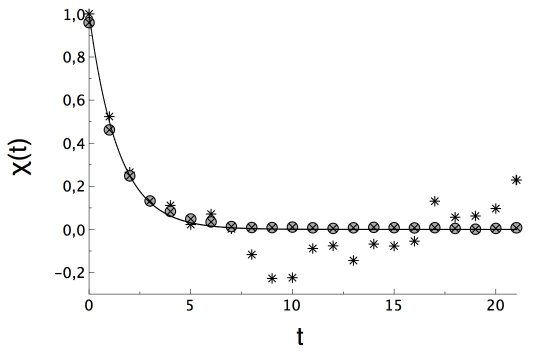
Figure 1: The impulse response of system (11)-(16) is given by $\chi(t)=2^{-t}$ (solid line). It is compared with numerical simulations using the estimate (19) (with $\epsilon=0.01,N=4552000$, symbol “*” ). In this example, it is seen that large fluctuations grow from $t=8$. The other points ( symbol “x”) are obtained by using the indirect method which consists in calculating the (inverse) Fourier transform of estimate (21) (See also Fig.2).

In ref. [5] the authors discuss the growth of the error due to finite size sampling and show that it grows faster than $\exp(\lambda t)/\sqrt{N}$ where $\lambda$ is the largest Lyapunov exponent (here $\lambda=\log 2$). This difficulty is enhanced in computing the susceptibilty $\hat{\chi}(\omega)$, as this Fourier transform needs a long time estimate of (19). Therefore in [8] we have developed a new method which takes the other way round. We compute numerically the susceptibility and, if needed, deduce from it the impulse response.

The principle of the new procedure we have implemented is quite simple [16]: returning to the system (11), we know that the average $<A>_{t}$ differs from $<A>=\pi$ by $<\delta A>_{t}=\epsilon\hat{\chi}(\omega)e^{-i\omega t}$. So $\hat{\chi}(\omega)=<\delta A>_{t}e^{i\omega t}/\epsilon$ is independent of $t$ and we can write for arbitrary large $T$:

$$\hat{\chi}(\omega)=\frac{1}{T\epsilon}\sum_{t=1}^{T}<\delta A>_{t}e^{i\omega t}$$ (20)

Let us remark that in this equation $<\delta A>_{t}=<A>_{t}-<A>$ represents a complex number because the perturbed dynamics given by (11) is written by means of the complex perturbation $\epsilon\xi(\theta)e^{-i\omega t}$. In practise, however, i.e. for numerical purpose, $<A>_{t}$ can be decomposed in real and imaginary parts, $<A>_{t}=<A_{1}>_{t}+i<A_{2}>_{t}$, and both of them can be computed separately by considering respectively perturbation of the forms $\epsilon\xi(\theta)\cos(\omega t)$ for $<A_{1}>_{t}$ and of the form $-\epsilon\xi(\theta)\sin(\omega t)$ for $<A_{2}>_{t}$. Now the important point is that the above average $<\;>_{t}$ could be attained also by making use of an ergodic assumption. In other words, for a fixed $\omega$ the time-periodic SRB measure underlying the average $<\;>_{t}$ can be created by the long time evolution of the perturbed system. Therefore we can estimate (20) by writing, for $\omega\neq 0$, small $\epsilon$ and sufficiently long $T$:

$$\hat{\chi}(\omega)\approx\frac{1}{T\epsilon}\sum_{t=1}^{T}A(\tilde{f}^{t}(\theta))e^{i\omega t}$$ (21)

where $\tilde{f}$ is the perturbed dynamics given by (11), modulo its practical implementation in terms of real and imaginary parts. Let us notice that in the latter sum we can replace $\delta A$ by $A$ because the contribution of the non-perturbed dynamics in this average disappears (for $\omega=0$).

Our numerical methods allows one, in principle, to compute the susceptibility $\hat{\chi}(\omega)$ for an arbitrary sampling of $\omega=k2\pi/M\in[0,2\pi]$. The subsequent inverse Fourier transform can then provide the impulse response on the time interval $[0,M]$ with large $M$. This procedure has been used with success in [8, 11]. Here we illustrate it on the basic example considered above. Figure 2 shows comparison of the analytical result of eq. (18) with the numerically computed susceptibility, which is quite satisfactory.

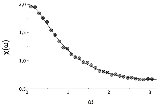
Figure 2: Modulus of the complex susceptibility as computed analytically [from eq. (18), solid line] and numerically [symbol “x”]. The latter is given by the estimate (21) averaged over $200$ samples obtained with $\epsilon=0.01$ and $T=2^{19}$.

Note that both approximation relations (19)-(21) do not involve an explicit linearisation (or a differentiation) of the dynamics. Therefore these relations can be used to numerically tackle the nonlinear response of the system to perturbations. From the operational point of view, the linear regime is characterised by a non-dependence of the results in $\epsilon$.

NB: To obtain these numerical results we had to iterate the dynamics $\theta_{t+1}=2\theta_{t}\mbox{\rm mod}\>2\pi$ and it is well known that a naive simulation of this map eventually drives all trajectories to $0$. We have circumvented the problem by encoding numbers with an (arbitrary long) sequence of bytes and used the left shift $<<$ available in $C$ language. This shift set the last bit to zero. Then we replace it by a bit $0$ or $1$ randomly chosen with a probability $p$ or $q$. For $p=q=\frac{1}{2}$ we obtain then trajectories typical for the SRB measure. Note that we can obtain trajectories typical for any Bernoulli measure by changing the probabilities $p,q$. We believe that this method is well known, though we haven’t been able to find any reference dealing with it.

3.3 Dealing with the non-invertibility of $f$

Now we come back to the general case where the perturbation $\xi(\theta)$ cannot be written as $(X\circ f)(\theta)$. Then, the change of variable $\phi=f(\theta)$ used in the integral (12), can still be performed, provided that the integration domain $[0,2\pi]$ is decomposed into the subintervals $[0,\pi]$ and $[\pi,2\pi]$ where $f$ is invertible. In this way the same formal expression (13) for $\chi(t)$ is obtained as before, but where:

$$X(\theta)=\frac{1}{2}\left[\xi(\frac{\theta}{2})+\xi(\frac{\theta}{2}+\pi)\right]$$ (22)

Thus in the chosen example, the effective perturbation $X(\theta)$ appears as the perturbation $\xi$ averaged over the pre-images of $f$. This concept generalises to general one-dimensional map $f$ defined on an interval $I=\bigcup_{k}I_{k}$ assuming the restrictions of $f$ to each $I_{k}$ invertible (say $f_{k}$) by writing :

$$X(\theta)=\sum_{k}\frac{\xi_{k}(\theta)\eta_{k}(\theta)}{|f^{\prime}(f_{e}^{-k}(\theta)|}\chi_{I_{k}}((f_{e}^{-k}(\theta))$$

where $\chi_{I_{k}}(\theta)$ is the indicatrix of interval $I_{k}$; $\xi_{k}=\xi\circ f_{e}^{-k}$ and $\eta_{k}=\eta\circ f_{e}^{-k}$, assuming that the SRB measure is written $\rho_{f}(d\theta)=\eta(\theta)d\theta$. Again a concrete example is easy to work out in the case of model 1. Let us choose $\xi(\theta)=\theta(2\pi-\theta)$. Then eq. (22) becomes $X(\theta)=\theta(2\pi-\theta)/2-1/4$ and it is found that $\chi(t)$ exactly as eq. (17) but divided by $4$.

4 Chaotic rotator in the plane

In the previous Section we have seen that in the case of systems with expanding dynamics only the fluctuation-response theorem applies: under suitable hypothesis, the response functions are matched with correlation functions. In view of the simple examples treated above, the technical point which makes the result work is integrating by part in eq. (8) (and in example eq. (12)). In the general case this integration by part is no longer possible (in the stable directions) for hyperbolic dynamics with contraction in phase space. This is because the SRB measure becomes usually singular in the stable directions so that it cannot be written with a density function, e.g. $\rho_{F}(d{\bf x})\neq\eta({\bf x})d{\bf x}$ for some regular function $\eta({\bf x})$. Nevertheless the response function given by the integral (8), and so the susceptibility, can be well defined, but in general cannot be identified anymore with a correlation function. To analyse this situation, Ruelle decomposes the perturbation giving rise to the response functions in two parts, by locally projecting this perturbation respectively onto the stable and the unstable directions of the tangent dynamics. This can be achieved when the system is uniformly hyperbolic, i.e. when the tangent space at any point ${\bf x}$ decomposes uniformly with respect to ${\bf x}$ into a direct sum of a stable and an unstable subspace (e.g. [9]).

The goal of this Section is to illustrate this decomposition on simple models where the uniform hyperbolicity holds by construction and where explicit computations can be done. To this purpose we consider a class of two-dimensional hyperbolic systems with a chaotic attractor on the unit circle, as represented on figure 3. Here the phase space is represented by the plane which is contracted by the dynamics onto the unit circle where there is a rotation with expanding dynamics. This might be one of the simplest example representing a chaotic (non-fractal) attractor. There are several ways to implement this qualitative dynamics, the simplest one being to decouple the rotation and the radial contraction. In all the forthcoming implementations of this class of model, one assumes that the SRB measure can be factorised as a product of the form:

$$\rho_{F}(dxdy)=\rho_{F}(rdrd\theta)=\delta(r-1)rdr\,\eta(\theta)d\theta/2\pi$$

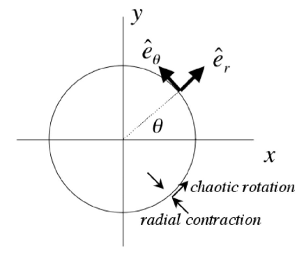
Figure 3: Schematic representation of the phase portrait of the toy model. The phase plane is shrinked by the dynamics on the unit circle playing the role of the chaotic attractor. Models implementing this scheme are given by eqs. (28).

Here $\delta(r-1)$ is the singular part of the measure, due to the contraction of the radial direction. On the other hand the measure on the unit circle (which represents the unstable manifold of any point on the attractor) is continuous and described by the density function $\eta(\theta)$. The latter is equal to $1$ in the particular case of the dynamics $\theta\mapsto 2\theta$ considered in the previous Section. Before specifying some implementations of the dynamics of Fig. 3, we summarize the objective of the linear response theory and introduce the notations as follows. Consider the 2-dimensional time-discrete systems:

$$x_{t+1} = F_{x}(x_{t},y_{t})+\epsilon_{x}\,\xi_{x}(t+1,x_{t},y_{t})$$

$$y_{t+1} = F_{y}(x_{t},y_{t})+\epsilon_{y}\,\xi_{y}(t+1,x_{t},y_{t})$$ (23)

where the first term ${\bf F}=(F_{x},F_{y})$ is the (autonomous) dynamics which is perturbed by a time-dependent vector field of small amplitude ($\epsilon=|(\epsilon_{x},\epsilon_{y})|\ll 1$). Here the coordinates $(x,y)$ do not necessarily mean the cartesian coordinates, but general coordinates on the plane. In the following, we will consider only two cases, however, namely the cartesian or the polar coordinates. Furthermore, the observables will be the coordinates themselves, except for the “angle” variable of the polar coordinates which will be chosen like previously as $A(\theta)$, i.e. the projection of $\theta$ in $[0,2\pi)$.

Now suppose that in absence of perturbation the mean values of $x$ and $y$ are zero. Then, when the perturbation is turned on, we are interested to the mean values of $(x_{t},y_{t})$ to first order in $\epsilon$. When $\mbox{{\boldmath$\xi$}}(t,x,y)=\mbox{{\boldmath$\xi$}}(x,y)e^{-i\omega t}$, the solution of this problem has been discussed above and it can be written in terms of the susceptibility matrix, namely:

$$\left(\begin{array}[]{c}<\delta x>_{t}\\ <\delta y>_{t}\end{array}\right)=\left(\begin{array}[]{cc}\hat{\chi}_{xx}(\omega)&\hat{\chi}_{xy}(\omega)\\ \hat{\chi}_{yx}(\omega)&\hat{\chi}_{yy}(\omega)\end{array}\right)\left(\begin{array}[]{c}\epsilon_{x}\\ \epsilon_{y}\end{array}\right)e^{-i\omega t}$$ (24)

The matrix elements $\hat{\chi}_{ij}(\omega)$ ($i,j=x$ or $y$) are the Fourier transform of the impulse response matrix elements given by eq. (8) :

$$\chi_{ij}(t) = \int\rho_{F}(dxdy)\nabla F_{i}^{t}(F({\bf x}))\cdot(\xi_{j}({\bf x}){\bf e}_{j})$$ (25)

$$= \int\rho_{F}(dxdy)\nabla F_{i}^{t}({\bf x})\cdot(X_{j}({\bf x}){\bf e}_{j})$$

In the last equation the function $X_{j}$ coincides with $\xi_{j}\circ{\bf F}^{-1}$ if the dynamics is invertible. If ${\bf F}$ is not invertible then, as discussed in the previous Section, $X_{j}$ can be interpreted as a type of averaging of $\xi_{j}$ over the pre-images of ${\bf F}$.

Finally, assuming that the system is uniformly hyperbolic, i.e. when the tangent space at ${\bf x}$ decomposes uniformly into a direct sum of a stable and an unstable subspace, the vector $X_{j}({\bf x}){\bf e}_{j}$ appearing in (25) will be decomposed as

$$X_{j}({\bf x}){\bf e}_{j}={\bf X}_{j}^{s}+{\bf X}_{j}^{u}$$ (26)

Then, by substituting this sum in eq. (25) we will be mostly interested in the ensuing decomposition of $\chi_{ij}(t)$ into the stable and unstable susceptibilities as follows:

$$\chi_{ij}(t) = \chi_{ij}^{(s)}(t)+\chi_{ij}^{(u)}(t)$$ (27)

for $t\geq 0$ (and $\chi_{ij}=0$ otherwise).

In what follows we start by considering the cases where by construction ${\bf X}_{j}^{u}=0$ or ${\bf X}_{j}^{s}=0$ in eq. (26). This enables one to concentrate on the stable or on the unstable susceptibilities and their resonances, the former being the novel feature of out of equilibrium dissipative systems.

4.1 Stable resonances

As a first realisation of the phase portrait depicted on Fig. 3, we use polar coordinates (i.e. $x\equiv\theta$ and $y\equiv r$ in the eqs. (23)) and we consider the following system:

$$\theta_{t+1} = g(\theta_{t},r_{t})+\epsilon_{\theta}\,\xi_{\theta}(t+1,\theta_{t},r_{t})$$

$$r_{t+1} = R(r_{t})+\epsilon_{r}\,\xi_{r}(t+1,\theta_{t},r_{t})$$ (28)

with $g(\theta)=2\theta+b(r-1)$ ($b$ constant) and $R(r)=1+e^{-\mu}(r-1)$, with $\mu>0$.

We first rule out the case $b=0$. Then the angular dynamics is the same as before, $g(\theta)=2\theta$, and the system becomes extremely simple because the radial and the phase dynamics are decoupled. The radial dynamics is trivially contracting on the unit circle, with $r_{t}=R^{t}(r_{0})=1+e^{-\mu t}(r_{0}-1)$. Also, the impulse response matrix is diagonal, because $\hat{\chi}_{r\theta}(\omega)=\hat{\chi}_{\theta r}(\omega)=0$ which is readily deduced from eq. (25). Using the same equation, the diagonal elements are computed as follows:

$$\chi_{\theta\theta}(t) = \int\!\rho_{F}(rdrd\theta)\,\partial_{\theta}f^{t}(\theta)\,X_{\theta}(\theta,r)=-<\theta_{t}\,;\partial_{\theta}X_{\theta}(\theta_{0},1)>$$ (29)

$$\chi_{rr}(t) = \int\!\rho_{F}(rdrd\theta)\,\partial_{r}R^{t}(r)\,X_{r}(\theta,r)=e^{-\mu t}<X_{r}(1,\theta)>$$ (30)

for $t\geq 0$. The first line is identical to the response function (15) obtained for the basic model studied in the preceding Section. This unstable response function, corresponding to perturbation parallel to the attractor, is thus a correlation function. As an illustrative example we can calculate these integrals in the case of perturbation function $\xi_{r}(t,\theta,r)=\xi_{\theta}(t,\theta,r)=X(\theta)\delta_{t0}$, where $X(\theta)$ is chosen as before (cf. eq. (16)). Then the susceptibility $\hat{\chi}_{\theta\theta}(\omega)$ is given explicitly by eq. (18). One notices that it possesses a pole in $\omega=-i\log 2$. On the other hand, eq. (30) is an example of stable response, i.e. the response to a perturbation along the contracting direction of the attractor. Note that the result is calculated without integration by part. The corresponding susceptibility is then computed as:

$$\hat{\chi}_{rr}(\omega)=\frac{C}{1-e^{i(\omega+i\mu)}}$$ (31)

where $C$ is a constant. Now this function has a pole located on the imaginary axis in $\omega=-i\mu$. This pole is independent of the ones of the correlation function. In particular it can be situated arbitrarily close to the real axis. This simple example clearly shows the effect of two types of perturbation on the system, either transverse or parallel to the attractor.

Let us deal with the case $b\neq 0$, which introduces a skew dynamics between the stable and the unstable variables. Then, if one starts with an initial condition $(\theta_{0},r_{0})$ the angular dynamics is easily worked out, giving the following expression :

$$\theta_{t}=g^{t}(\theta,r)=\left(2^{t}\theta+b(r-1)\frac{2^{t}-e^{-\mu t}}{2-e^{-\mu}}\right)\>(\mbox{\rm mod}\>2\pi)$$ (32)

Let us notice that the dynamics on the attractor ($r=1$) is the same as before. This implies that the diagonal terms of the susceptibility remains the same as for $b=0$, and the correlation functions do not change. However, the dependence of $g^{t}$ on $r$ creates now a non-diagonal term which can be written as follows:

$$\chi_{\theta r}(t)=b\frac{2^{t}-e^{-\mu t}}{2-e^{-\mu}}\,B(t)\quad\quad\mbox{\rm with}\quad B(t)=\int_{0}^{2\pi}\!X(\theta)\,d\theta-\sum_{k=1}^{2^{t}}X(k\frac{2\pi}{2^{t}})2^{-t}$$ (33)

Let us remark that the factor $B(t)$ can be interpreted as an “error” function measuring the difference between the integral of $X(\theta)$ and its approximation by a Riemann sum with intervals $2^{-t}$. (This factor $B(t)$ stems from the distribution derivative of the “angle” observable eq. (3) ). It is clear that if $X(\theta)$ is Riemann integrable, then the “error $B(t)$ has to decrease to zero when $t$ becomes large. Actually, in view of eq. (33) it should decrease faster than $2^{-t}$ to get $\chi_{\theta r}(t)$ going to $0$ with $t$ large. For example in the case of $X(\theta)$ given by eq. (16), we obtain $B(t)=2^{-2t}$ and thus

$$\chi_{\theta r}(t)=b\frac{2^{-t}-e^{-(2\log 2+\mu)t}}{2-e^{-\mu}}$$ (34)

This geometrical interpretation of function $B(t)$ shows directly that if $X(\theta)$ varies much in $[0,2\pi]$ then it will take a long time $t$ to reach an actual exponential decrease of $B(t)$. By the meantime the response function can transiently grow a lot due to the exponential factor $2^{t}$. Therefore the degree of variation of $X(\theta)$ determines the transient growth of the stable response function. This property will be used later in Section 4.4 by considering a perturbation function of the form $X(\theta)=\cos(2^{p}\theta)$.

Now, the susceptibility $\hat{\chi}_{\theta r}(\omega)$, which can be readily deduced from (34), possesses a pole situated in $\omega=-i(2\log 2+\mu)$ on the imaginary axis. The $\mu$ contribution is clearly due to the contracting dynamics, whereas the first term $2\log 2$ is in fact a Ruelle-Policott resonance (in the present case they are multiples of $\log 2$). Thus this example shows a new feature which can appears when the variables are not trivially decoupled into stable and unstable variables: some stable resonances become a (linear) combination of poles due to the contracting direction and of resonances belonging to the correlation functions. An attempt of generalisation of this property is given in the Appendix.

4.2 Stable resonances with arbitrary frequencies

The elementary model described by eq. (28) has only a one-dimensional radial dynamics. Consequently any stable pole of the corresponding susceptibility will be located along the imaginary axis. On the other hand it is possible to generalise this model in order to show that stable poles can have arbitrary frequencies and relaxation times. It suffices to increase to number of degrees of freedom of the system. To illustrate this point we present in this section two examples for which the stable resonances can have arbitrary non zero frequencies.

A simple way to add more degrees of freedom to the radial dynamics is to transform its dynamics into a higher order reccurence. For instance let us consider a new type of rotator whose equations are a variation of system (28) taking the form:

$$\theta_{t+1} = g(\theta_{t},r_{t})$$

$$r_{t+1} = R(r_{t},r_{t-1})$$ (35)

with as before $g(\theta)=2\theta+b(r-1)$ but now $R(r,\varrho)=1+2e^{-\mu}\cos(\omega_{0})(r-1)-e^{-2\mu}(\varrho-1)$ ($\mu>0$). The choice of this dynamics is motivated by the fact that it creates in the stable susceptibility a pole placed simply at $\omega_{0}-i\mu$. Thus we can easily control its frequency by varying $\omega_{0}$. This example is easy to deal with because the radial dynamics can be solved exactly, and it can be checked that given $r_{0}$ arbitrary and $r_{-1}=0$, one gets:

$$r_{t}=1+(r_{0}-1)e^{-\mu t}\sin\omega_{0}(t+1)/\sin\omega_{0}$$ (36)

This case will be considered below in cartesian coordinates.

Another way to increase the number of degrees of freedom is to consider a network of interconnected rotators. This example is interesting because it has links with the chaotic network model that we have studied previously [8, 11] and which is mentionned in the introduction of this paper. So we consider now a collection of $N$ interconnected rotators of the same type as before (cf. fig. 3), assuming for simplicity that the coupling between the units occurs only by means of their radial variables. The equations of this model are the following:

$$\theta_{i,t+1} = g(\theta_{i,t},r_{i,t})$$

$$r_{i,t+1} = 1+\sum_{j=1}^{N}J_{ij}(r_{j,t}-1)$$ (37)

where $i\in\{1,\cdots,N\}$ denote the index of the i^th rotator in the network. The function $g(\theta,r)=2\theta+b(r-1)$ is the same as before and the real numbers $J_{ij}$ form a matrix J. The only requirement about this matrix is that its spectrum lies inside the unit circle such that it gives in fact a contraction of the radial variables onto $r_{i}=1$ for any $i$. On the other hand we can interpret J as the connectivity matrix of the network, meaning that the rotator $j$ influences rotator $i$ iff $J_{ij}\neq 0$. Moreover this interaction is signed, with the interpretation that positive $J_{ij}$ means activation and inhibition is described by negative $J_{ij}$.

The model (37) is a straightforward generalisation of system (28), so that the explicit time evolution for $(\theta_{i,t},r_{i,t})$ can also be calculated. Furthermore, if J is diagonalisable, with $\mbox{ \sf P}^{-1}\mbox{ \sf J}\mbox{ \sf P}=diag\{e^{-\mu_{1}+i\omega_{1}},\cdots,e^{-\mu_{N}+i\omega_{N}}\}$ , then the stable complex susceptibilities (with respect to a perturbation of amplitude $\epsilon X(\theta)$ in the $r_{j}$ direction as considered in the single rotator model) can be expressed as follows:

$$\hat{\chi}_{r_{i}r_{j}}(\omega) = \sum_{k}\frac{P_{ik}P^{-1}_{kj}}{1-e^{i(\omega-\omega_{k})-\mu_{k}}}$$

$$\hat{\chi}_{\theta_{i}r_{j}}(\omega) = \sum_{k}P_{ik}P^{-1}_{kj}(\frac{1}{1-e^{i\omega-\log 2}}-\frac{1}{1-e^{i(\omega-\omega_{k})-(2\log 2+\mu_{k})}})$$ (38)

So, it is readily seen that there are stable poles situated in the lower half-complex plane in $\omega=\omega_{k}-i\mu_{k}$ and in $\omega=\omega_{k}-i(2\log 2+\mu_{k})$, each time $e^{-\mu_{k}+i\omega_{k}}$ is an eigenvalue of matrix J. Therefore, although in this model the unstable resonances are located only on the imaginary axis, depending on the connectivity matrix there can be an arbitrary number of stable resonances with non-zero frequencies $\omega_{k}$. The latter will not be visible in the power spectrum of the chaotic dynamics, but eqs. (38) shows that a periodic forcing of unit $j$ at frequency $\omega_{k}$ can produce a resonance in the linear response of unit $i$. As discussed in ref. [11], this property can be used to transmit a signal from $j$ to $i$ (possibly with amplitude modulation). Moreover we see that a necessary condition to make this transmision possible is that $P_{ik}P^{-1}_{kj}\neq 0$. This condition is satisfied if the $k^{th}$ eigenmode of J has a nonzero component $i$ in the canonical basis and reciprocaly if the $j^{th}$ vectors of that canonical basis has a nonzero component $k$ when decomposed in the eigenvector basis. (Roughly speaking, an excitation of the node $j$ excites the eigenmode $k$, which excites the node $i$). This opens the possibility, for appropriately chosen connectivity matrices J, to get resonances which are specific to the pair $ij$. Note in particular that if the network as some modular structure such that the matrix $\sf P$ has a block diagonal structure then, obviously, there are resonances specific to each block. This structure is revealed by our excitation-response procedure even when one has no access to the explicit form of the dynamics.

4.3 Relaxation time longer than the mixing time

To summarise, in the previous sections we have seen that the linear response between two variables $(x_{i},x_{j})$ of a uniformly hyperbolic system can be characterised by poles of its susceptibility $\hat{\chi}_{ij}(\omega)$. A given pole $\omega=\omega_{k}-i\mu_{k}$ of this function is associated with two time scales, namely its resonance frequency $\omega_{k}$ and its relaxation time $\mu_{k}^{-1}$. The latter gives an estimation of the decay time of oscillations $\omega_{k}$ when the system is submitted to an impulse perturbation via its $x_{j}$ variable. Moreover, in view of the decomposition $\hat{\chi}_{ij}(\omega)=\hat{\chi}_{ij}^{(u)}(\omega)+\hat{\chi}_{ij}^{(s)}(\omega)$ introduced in eq. (27), there can be two types of poles. The first class of poles are the ones of $\hat{\chi}_{ij}^{(u)}(\omega)$. They coincide with the Ruelle-Pollicott resonances, which are also the poles of the power spectrum of a generic variable of the chaotic system. The knowledge of the closest pole to the real axis in this class provides the mixing time $\tau_{m}$, defined as the inverse of its imaginary part. This is also the typical decay time of the correlation functions which can be interpreted as the “decorrelation” time of state variables of the chaotic attractor. In the basic examples treated above $\tau_{m}=1/\log 2$. The second class of poles is formed by the poles of the stable susceptibility $\hat{\chi}_{ij}^{(s)}(\omega)$. In particular their imaginary parts characterise the average decay time of an impulse perturbation along the stable direction, and thereby the average time to come back to “equilibrium” after this perturbation. For instance in the example of the previous Section, eq. (38) shows that the return time of $<\theta_{i}>_{t}$ to equilibrium after an impulse perturbation in the stable direction $r_{j}$ is dominated by the largest $\tau_{ij}=\max_{k}(2\log 2+\mu_{k})^{-1}$, ($k$ chosen in $\{1,\cdots,N$ such that $P_{ik}P^{-1}_{kj}\neq 0\}$). Thus in this example $\tau_{mixing}>\tau_{ij}$ for all pairs $ij$ and this corroborates the common belief that the return time to equilibrium of a physical system is given by its mixing time.

This property is not true in general, however. The goal of the present Section is to support this statement by providing a generalisation of our simple model (28) where indeed the decay of response functions can be much longer than the mixing time. Moreover since this property was already observed in our previous study of neural network dynamics [11], the present example indicates also a possible mechanism to understand this non-classical behaviour.

Let us consider the following system, which is an extension of system (28):

$$\theta_{t+1} = 2\theta_{t}+b(r_{t})(r_{t}-1)+(b(r_{t})-1)\sin\theta_{t}$$

$$r_{t+1} = 1+e^{-\mu}(r-1)$$ (39)

with $b(r)=e^{-(r-1)/\eta}$ and $\eta>0$. Thus in the neighborhood of $|r-1|\ll\eta$, the new term $(b(r_{t})-1)\sin\theta_{t}$ is negligible and the system then behaves exactly as the basic model of Section 4.1. This is no longer the case when $r-1$ increases, entailing that $b(r)$ decreases to $0$. Figure 4 shows the $\theta$ dynamics in the two limits $r=1$ and $r=\infty$.

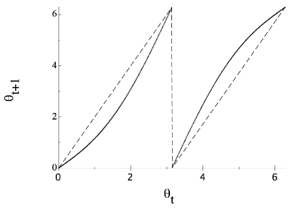
Figure 4: First return map representation of the $\theta$ dynamics defined by eq. (39) in the two limiting case $(r-1)\sim 0$ (dashed line) and $(r-1)\gg\eta$ (solid line).

This model is hardly tractable analytically because it is hard to compute $(\theta_{t},r_{t})$ as a function of $(\theta_{0},r_{0})$. But the dynamics can still be analysed by making use of the numerical method described in Section 3.2. Figure 5A shows a superposition of the susceptibilities $|\hat{\chi}_{\theta r}(\omega)|$ obtained from two numerical computations performed with two different values of $\eta$. For $\eta=1$ in eqs. (39), the numerical results can be well fitted with the analytical curve computed in the case $\eta=\infty$ (i.e. the Fourier transform of eq. (38) or, equivalently eq. (34) in the case of only one unit). Then the width of the resonance in $\omega=0$ is dominated by $\log 2$ corresponding to the inverse of the mixing time.

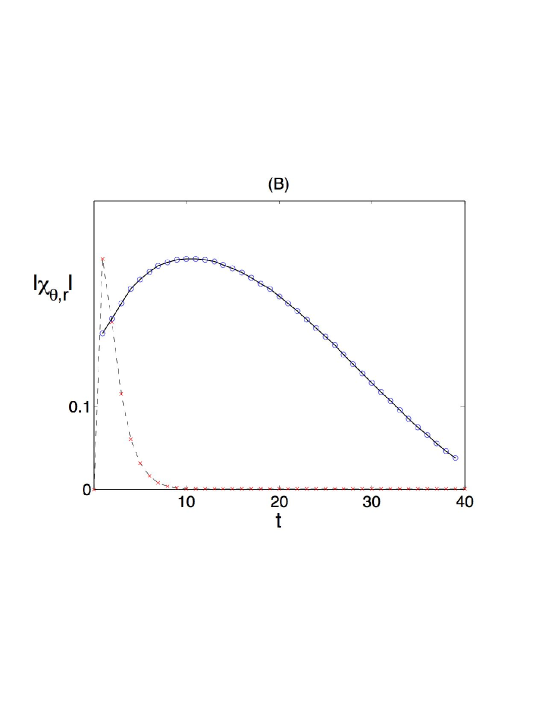
Figure 5: (A) Modulae of the susceptibility $\hat{\chi}_{\theta r}(\omega)$ computed for the model (39) for different values of $\eta$. The dashed line curve is the analytical prediction of $|\hat{\chi}_{\theta r}(\omega)|$ in the case $\eta=\infty$. The case $\eta=0.05$ (symbol ‘o’ ) is numerically computed with estimate (21) ($\epsilon=0.01,T=2^{19}$ and yet averaged over $200$ samples). It shows a remarkable narrowing of the peak. (B) Impulse response functions $\chi_{\theta r}(t)$ computed from the inverse Fourier transform of $\hat{\chi}_{\theta r}(\omega)$. In both cases (A) and (B) the height of curves $\eta=\infty$ have been scale to the same amplitude than $\eta=0.05$.

On the other hand the narrower curve (with symbols “x”) in fig. 5 shows an example of $|\hat{\chi}_{\theta r}(\omega)|$ computed for small $\eta$. In this case it is seen that the width of the resonance in $\omega=0$ has substantially decreased. As a matter of fact it can be arbitrarily decreased by diminishing further $\eta$. In the same time the height of the resonance peak increases. (This is not visible on the figure because their maxima have been scaled to the same height). Thus the susceptibility $\hat{\chi}_{\theta r}(\omega)$ diverges with $\eta\rightarrow 0$ because one of its poles pinches the real axis in this limit. The reason for this behavior can be understood at least qualitatively as follows. As $r-1$ increases from $\eta$, the system (39) looses indeed its uniform hyperbolicity. This is clear on fig. 4, where it is seen that it $r-1\gg\eta$ then the first return map for $\theta_{t}$ acquires a slope 1 in abscissa $\theta=0$. This means that a perturbation along the radial direction can induce a drastic slowing down of the “chaotic” rotation. The latter is resumed only when the radial perturbation has sufficiently relaxed. Thus in this case this is the decay time along the contracting direction which controls the return time to equilibrium.

Now one interesting physical consequence of this phenomenon appears by reconstructing the impulse response function $\chi_{\theta r}(t)$ from the inverse Fourier transform of $\hat{\chi}_{\theta r}(\omega)$. Figure 5B shows the comparison between the cases $\eta$ large (cf. eq. (34)) and $\eta$ small. In the first case the response of $\theta$ decays as expected like $2^{-t}$ which is the typical decay time of the correlation functions of this system. In the second case it is seen that the system responds with an impulse of large amplitude which moreover decays on a time of order 10 times longer than the mixing time. Therefore this example illustrates a novel feature of Ruelle’s theory, compared with the common intuition of nonequilibrium physical (conservative) systems: when a dissipative system is pushed out of equilibrium, its return time to equilibrium can be substantially longer than the mixing time which could be predicted by looking at its correlation functions. This property merely reflects the possible violation of the fluctuation-response theorem in dissipative systems.

The numerical simulations reported in this section concerned our single rotator which is a 2 degrees of freedom system. Nevertheless we anticipate that the same type of phenomenon will show up in the network of rotators described by eqs. (37). In fact this behaviour of having a longer return time to equilibrium than the mixing time was also observed in the numerical simulations of our neural network dynamics [11].

4.4 Decomposing the linear response in general coordinates

The model (28) is sufficient to show the existence of two types of responses in hyperbolic systems. However, the choice of variables $(\theta,r)$ made to perturb this system and to observe its response is quite particular because its coincides with the local unstable and stable directions $\{{\bf e}_{\theta},{\bf e}_{r}\}$. So the decomposition of the response functions, or of the susceptibilities, into their stable and unstable parts is trivial for this choice. In this Section, we analyse the same model, but with observables which are the cartesian coordinates in the plane. The unperturbed dynamics is thus the same but we change the way to perturb it and the variables to look at. The problem becomes slightly more complicated because each element of the the susceptibility matrix have both components, stable and unstable. The identification of these two contributions in a response function can scarcely be done explicitly in a general system because the projectors onto the local stable or unstable manifolds are not easy to compute for an arbitrary system. Nevertheless the present model is sufficiently simple to perform this decomposition analytically and to discuss some of its consequences on the resonances of the susceptibility.

Let us consider the model (35) introduced before but now written in cartesian coordinates $(x,y)$ of the plane:

$$x_{t+1} = F_{x}(x_{t},y_{t},x_{t-1},y_{t-1})+\epsilon_{x}\,\xi_{x}(t+1,x_{t},y_{t})$$

$$y_{t+1} = F_{y}(x_{t},y_{t},x_{t-1},y_{t-1})+\epsilon_{y}\,\xi_{y}(t+1,x_{t},y_{t})$$ (40)

with the functions ${\bf F}=(F_{x},F_{y})$ defined by:

$$F_{x}(x_{t},y_{t},x_{t-1},y_{t-1}) = R(\sqrt{x_{t}^{2}+y_{t}^{2}},\sqrt{x_{t-1}^{2}+y_{t-1}^{2}})\cos(g[\arg(x,y),\sqrt{x_{t}^{2}+y_{t}^{2}}])$$

$$F_{y}(x_{t},y_{t},x_{t-1},y_{t-1}) = R(\sqrt{x_{t}^{2}+y_{t}^{2}},\sqrt{x_{t-1}^{2}+y_{t-1}^{2}})\sin(g[\arg(x,y),\sqrt{x_{t}^{2}+y_{t}^{2}}])$$ (41)

and the functions $R$ and $g$ have already been defined after eq. (35). The notation $\arg(x,y)$ means $\arctan(y/x)$ for $x>0$ and $\arctan(y/x)+\pi$ for $x<0$. Thus in the absence of perturbation ($\epsilon_{x}=\epsilon_{y}=0$), the standard change of variable $x=r\cos\theta$, $y=r\sin\theta$ gives the unperturbed model (35).

Assuming without loss of generality that the mean values of the variables are zero in the unperturbed situation, $<x>=0=<y>$, we are interested in the mean values $<x>_{t}$ and $<y>_{t}$ for small $\epsilon$ and a prescribed form of the perturbation function $\mbox{{\boldmath$\xi$}}(x,y)$. As already discussed (see footnote 5), in order to simplify the formalism we choose a perturbation the form $\mbox{{\boldmath$\xi$}}={\bf X}\circ{\bf F}$, with ${\bf X}=X_{x}{\bf e}_{x}$ or ${\bf X}=X_{y}{\bf e}_{y}$. The goal is now to compute the susceptibility matrix $\hat{\chi}_{ij}(\omega)$, or equivalently the corresponding response matrix ${\chi}_{ij}(t)$ defined in eq. (25), as well as its decomposition in a sum of an unstable and of a stable part. To this purpose, by construction in the present model the perturbation $X_{j}{\bf e}_{j}$ ($j=x$ or $y$) can be decomposed along its stable and its unstable projections, for example :

$$X_{y}{\bf e}_{y}=X_{y}\sin\theta\,{\bf e}_{r}+X_{y}\cos\theta\,{\bf e}_{\theta}$$ (42)

where ${\bf e}_{r}$ is the radial unit vector (local stable direction) and ${\bf e}_{\theta}$ is the tangential unit vector to the circle (local unstable direction). Thus from eqs. (25)-(27), and by using the equations $\nabla F_{i}.{\bf e}_{r}=\partial_{r}F_{i}$ and $\nabla F_{i}.{\bf e}_{\theta}=\frac{1}{r}\partial_{\theta}F_{i}$ ($i=x$ or $y$) , one can write the decomposition of $\chi_{xy}(t)$ into the stable and unstable susceptibilities as follows:

$$\chi_{xy}(t) = \chi_{xy}^{(s)}(t)+\chi_{xy}^{(u)}(t)$$

$$= \int\!\rho_{F}(d{\bf x})\,\sin\theta\,\partial_{r}F_{x}^{t}({\bf x})\,X_{y}({\bf x})+\int\!\rho_{F}(d{\bf x})\,\frac{\cos\theta}{r}\partial_{\theta}F_{x}^{t}({\bf x})\,X_{y}({\bf x})$$

for $t\geq 0$ (and $\chi_{xy}=0$ otherwise). The other matrix elements $\chi_{xx}(t)$ or $\chi_{yy}(t)$ have an anologous expression. Let us recall that the invariant measure to be used in these integrals takes the following form (in polar coordinates) : $\rho_{F}(d{\bf x})=rd\theta\,\delta(r-1)\delta(\varrho-1)drd\varrho$ with $\delta$ denoting here the Dirac distribution. This enables one to get the following results:

$$\chi_{xx}^{(u)}(t) = <\cos\theta_{t};\,\partial_{\theta}[\sin\theta_{0}X_{x}(\theta_{0})]>$$ (44)

$$\chi_{xx}^{(s)}(t) = \partial_{r}R^{t}<\cos\theta_{t};\,\cos\theta_{0}X_{x}(\theta_{0})>$$ (45)

$$\chi_{xy}^{(u)}(t) = -<\cos\theta_{t};\,\partial_{\theta}[\cos\theta_{0}X_{x}(\theta_{0})]>$$ (46)

$$\chi_{xy}^{(s)}(t) = -\partial_{r}g^{t}<\sin\theta_{t};\,\sin\theta_{0}X_{y}(\theta_{0})>$$ (47)

(We do not write the corresponding functions $\chi_{yy}^{(u)}(t)$ and $\chi_{xx}^{(u)}(t)$ which are quite similar). We have only considered a $\theta$-dependence of the perturbation function $X_{i}(\theta)$ (because a $r$ dependence would be trivial due to the Dirac distributions). As it is expected the unstable response functions (44) and (46) are pure correlation functions, whereas the stable responses (45) and (47) are correlation functions multiplied by a factor related to the contracting dynamics. As already discussed this latter term is responsible for creating poles in the susceptibility which are not observable in the powerspectrum.

Now, another point that we want to illustrate in this section is the following: as mentionned above, the decomposition $\chi_{ij}^{(s)}(t)+\chi_{ij}^{(u)}(t)$ can scarcely be done in practise. In this case the resonances which can be observed are induced from the maxima of the modulus $|\chi_{ij}(t)|$. But the latter can be misleading to detect actual poles of the stable or of the unstable susceptibilty. To make this point clearer, we treat a concrete example.

Let us consider again the perturbation function $X(\theta)=\theta(2\pi-\theta)$ to be used in eqs. (44)-(47) and let us compute explicitly $\chi_{xx}(t)=\chi_{xx}^{(u)}(t)+\chi_{xy}^{(s)}(t)$. The first term is given by the correlation function (44) which can be written as:

$$\chi_{xx}^{(u)}(t)=\int_{0}^{2\pi}\!d\theta\,\cos(2^{t}\theta)\partial_{\theta}[\theta(2\pi-\theta)\sin\theta]=\left\{\begin{array}[]{l}\frac{\pi}{2}+\frac{2}{3}\pi^{3}\mbox{\ \ if\ }t=0\\ -2\pi\left(\frac{1}{(2^{t}+1)^{2}}+\frac{1}{(2^{t}-1)^{2}}+\frac{2}{(4^{t}-1)}\right)\mbox{\ \ if\ }t>0\end{array}\right.$$ (48)

and, as usual, $\chi_{xx}^{(u)}(t)=0$ for $t<0$. Next we compute the stable susceptibility $\chi_{xx}^{(s)}(t)$ by evaluating the two factors of (45). The first factor $\partial_{r}R^{t}$ is worked out by using (36) and one gets

$$\chi_{xx}^{(s)}(t)=\frac{\alpha^{t}\,\sin\omega_{0}(t+1)}{\sin\omega_{0}}\,C(t)$$ (49)

with the second factor being the correlation function:

$$C(t)=\int_{0}^{2\pi}\!d\theta\,\cos(2^{t}\theta)\cos(\theta)\,\theta(1-\theta)=\left\{\begin{array}[]{l}-\frac{\pi}{2}+\frac{2}{3}\pi^{3}\mbox{\ \ if\ }t=0\\ -2\pi\left(\frac{1}{(2^{t}+1)^{2}}+\frac{1}{(2^{t}-1)^{2}}\right)\mbox{\ \ if\ }t>0\end{array}\right.$$ (50)

Finally the complex susceptibility is obtained by summing the stable and the unstable contributions. For example $\chi_{xx}(t)=\chi_{xx}^{(u)}(t)+\chi_{xx}^{(s)}(t)$ with eqs. (48)-(50).

In this example the poles of the complex susceptibility can thus be controlled by changing the parameters $\mu$ and $\omega_{0}$ which characterise the radial (thus here “transverse”) dynamics. Figure 6 shows the modulus of the complex susceptibility $|\hat{\chi}_{xx}(\omega)|$, as well as the respective contributions of the stable and the unstable susceptibilities, for a given choice of parameters $\alpha=0.8,\omega_{0}=1$.

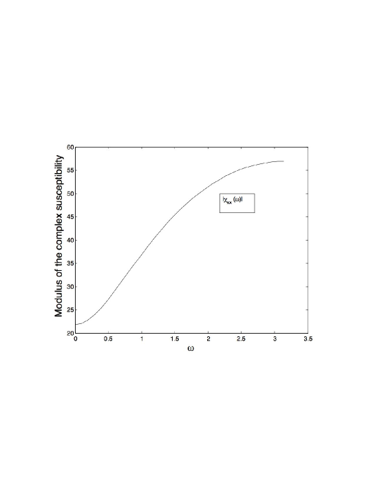
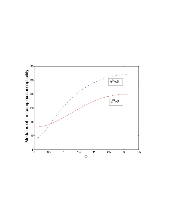
Figure 6: Complex susceptibility $\hat{\chi}_{xx}(\omega)$ computed from eqs. (48)-(50) with parameters $\alpha=0.8,\omega_{0}=1$. (a) Modulus of the complex susceptibility. (b) Modulus of the stable (solid line) and of the unstable (dashed-line) susceptibility.

For this choice one notices that the resonances exhibited by these curves are all situated in $\omega=\pi$. So in this case the information given by the Fourier transform of a correlation function, would suffice to characterise, at least qualitatively, the susceptibility of the system. In particular, the maximum response of the system to periodic forcing occurs at the same frequency that the resonance of correlation functions. This situation changes by tuning parameter $\omega_{0}$, however. Figure 7(a) shows a case where the resonance of the complex susceptibility is no longer situated in $\omega=\pi$, but near $\pi/2$.

As already discussed, this “anomalous” behaviour cannot be understood in the framework of the fluctuation-response theorem, but well in the Ruelle’s response theory of dissipative chaotic systems. On the other hand it can be remarked that the resonance of $|\hat{\chi}_{xx}(\omega)|$ near $\pi/2$ does not correspond to a stable nor to an unstable pole. In fact it results from the interference of two poles, stable and unstable, which appear as distinct resonances, which can be seen on the graph of $|\hat{\chi}_{xx}^{(s)}(\omega)|$ and of $|\hat{\chi}_{xx}^{(s)}(\omega)|$ represented on Fig. 7(b).

So this simple example illustrates that the linear response of the system depends on the behaviour or the “stable” response function. In particular this can drastically differ from all those of correlation functions. Moreover, one sees that the position of the stable poles can be tuned by controlling appropriate parameters ruling the dynamical systems.

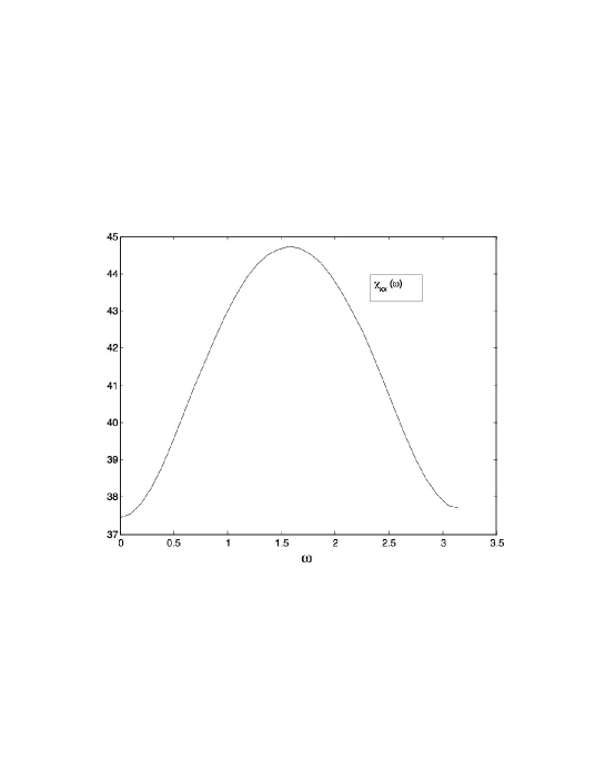
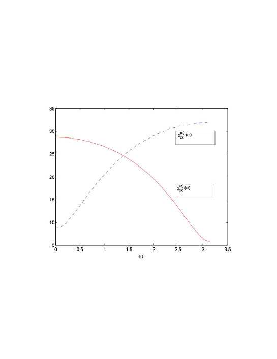
Figure 7: Complex susceptibility $\hat{\chi}_{xx}(\omega)$ computed from eqs. (48)-(50) with parameters $\alpha=0.8,\omega_{0}=3$. (a) Modulus of the complex susceptibility. (b) Modulus of the stable (solid line) and of the unstable (dashed-line) susceptibility.

Amplified echo of the impulse response

We end this Section by reporting another property of the stable response which is an application of the analytical results (44)-(47). The following result is also linked to the interpretation by mean function $B(t)$ [eq. (33)] of the transient growth of response functions, as discussed in Section 4.1.

The response function $\chi_{xy}^{(s)}(t)$ is a product of an exponential function and of a correlation function. If the latter is of amplitude of order (1) at time $t$, the result gives an amplification of $2^{t}$. To illustrate this property consider a perturbation of the form:

$$X(\theta)=\cos(2^{p}+1)\theta$$ (51)

Then is easy to work out the correlation function $<\sin\theta_{t}\,\sin\theta_{0}X_{y}(\theta_{0})]>$ appearing in (47). It is found that if $p>1$, the stable response function is

$$\chi_{xy}^{(s)}(t)=-\frac{b(2^{p}-e^{-\mu p})}{4(2-e^{-\mu})}\,\delta_{t,p}$$ (52)

Notice that in this case the susceptibility $\hat{\chi}_{xy}^{(s)}(\omega)\propto e^{ip\omega}$ has no poles. However, it is seen in this example that an effect of the stable direction is to produce an exponentially amplified ”echo” of the perturbation.

5 Conclusion

In the recent theory developed by Ruelle [4] the standard concepts of linear response, susceptibility and resonance are revised and extended due to the dynamical contraction of the whole phase space onto attractors. More technically, the contraction rate of phase space leads one to replace the conservative Liouville measure (which is the standard measure in classical statistical physics) by the notion of SRB measure. Among others, this change demands to go beyond the standard frawework of the “fluctuation-response” theorem, which means that one cannot any longer deduce the statistical behaviour of the system just by looking at its correlation functions. For example, the powerspectra of classical (conservative) physical systems provide in general all the informations about the resonances of this system. For the dissipative systems considered by Ruelle, this information is incomplete, however, as they may be new types of resonances –called the stable resonances because they are related to stable manifolds– which cannot be detected in the spectra of correlation functions but in the complex susceptibility of this system. In previous papers we have exhibited a model of dynamical network with dissipative chaotic dynamics where we succeeded to numerically compute the susceptibility and show indeed the presence of new resonances in the susceptibility which are absent in the Fourier transform of the correlation functions. In order to gain more intuitions on what bring about these “stable” resonances and their consequences, we have considered in the present article simpler models which could be treated analytically. Moreover the analytical results could be used to test further our numerical method and to compare it to a previous method which existed in the litterature.

We have first examined the 1-dimensional model $\theta_{t+1}=2\theta_{t}$ (mod $2\pi$) which presumably is the simplest chaotic system with Lyapunov exponent $\log 2$. Despite its simplicity this model is instructive to consider, as it is a non classical physical systems (having a purely expanding and non invertible dynamics). The linear response of this system can be worked out analytically and the result is a correlation function. In this case it is easy to show that this response decays exponentially with a characteristic time equal to the mixing time. Also the latter is clearly associated with a pole of the susceptibility and also identified with one Ruelle-Policott resonance.

Next we have studied a class of 2-dimensional models describing simple rotator models. The angular dynamics is the same as previously but there is also a radial dynamics which contracts the phase space on the unit circle (fig. 3). The resulting system has thus a non-fractal chaotic attractor, which moreover is uniformly hyperbolic. This elementary model could be used to illustrate several new properties associated with the dissipative dynamics. First it is easy to show in it the presence of new poles whose real parts correspond again to zero-frequency resonances but imaginary parts are associated with the relaxation time of the contracting dynamics. In fact it is seen that the cross-response $\hat{\chi}_{\theta r}(\omega)$ has a pole which combines the two characteristic times (mixing and contracting) in a linear combination of both. This property is demonstrated to exist in a class of more general and higher dimensional systems, as presented in the Appendix. In the rotator model one could also describe the stable resonance of $\hat{\chi}_{\theta r}(\omega)$ by means of the error function $B(t)$, eq. (33), showing how the analytic properties of the perturbation function $X(\theta)$ regulates the amplitude growth and decay of the response. Next we extended the calculations obtained for a single rotator to results for a network of coupled rotators. This generalisation pointed out to the possibility to get stable resonances wich are specific to the pair $ij$ in the network and having arbitrary non zero frequencies. Both of these features can be shown to be intimately linked to the spectral properties of the connectivity matrix of the network. This properties would be worth to analyse further as they are also related to the ability of the system to propagate signals between units of the network [11].

We have also considered an extension of the rotator model in another direction which allows one to discuss the relation between the return time to equilibrium of the system after an impulse perturbation and the mixing time. These characteristic times coincide when there is no attractor in the phase space but here we proposed a mechanism to get a relaxation time arbitrary long in case of transverse perturbation to the attractor. Roughly speaking it is enough that the transverse dynamics becomes less contracting with the distance to the attractor leading possibly to the loss of hyperbolicity for critical perturbations. More precisely we have implemented such mechanism in model (39) which presumably is beyond the scope of analytical treatment, but could be dealt with numerical simulations. These numerical results indeed showed the narrowing of stable resonances following our qualitative predicitions.

Finally we have analysed the simple rotator model in cartesian coordinates, illustrating a rare case where the decomposition of the susceptibility $\hat{\chi}_{ij}(\omega)=\hat{\chi}_{ij}^{(s)}(\omega)+\hat{\chi}_{ij}^{(u)}(\omega)$ in respectively stable and unstable components can be performed analytically. This example showed in particular that in some cases a maximum in the amplitude $|\hat{\chi}_{ij}(\omega)|$ may not be interpretable simply as a stable or an unstable pole, but rather as an interference effect of both.

The results obtained in this paper gives more insights in our previous work concerning the linear response of a chaotic network model [8]. This preceding study had allowed us to numerically demonstrate the existence of the new resonances predicted by Ruelle in a model of neural network. Thanks to a numerical method devised to compute the susceptibility and to extract also some poles of it, these new resonances were observed with the unexpected features to be often narrow and pair $ij$-dependent. This last property enabled us also to propose a method of signal transmission bewteen the nework units by means of amplitude modulation of harmonic signals locked on the resonance frequencies [11]. Now the present work permits us to understand some mechanisms able to create such resonances with arbitrary frequencies and arbitrary widths, and the possibility to get pair-selective resonances. In future works we will examine further how the control this pair selectivity and how pole positionning can be achieved so that we can propose more advanced schemes for communication between units within a chaotic network. We anticipate that such schemes would be quite useful not only in the field of neural networks but also for applications in other biological networks (e.g. gene regulatory networks) or in communication networks. In particular we will examine also ways of transmitting trains of periodic pulses, which are prevalent in the considered applications. On the other hand, to demonstrate the practical relevance of these new ideas we are working on experimental devices with dissipative chaotic dynamics in order to produce experimental evidences of the present linear response theory [17].

From the theoretical side it would be worth to deepen the consequences of the fractal (cantor-like) structure of generic strange attractors, a feature which was not considered in this paper. A generalisation of our rotator model would be to replace the contracting dynamics along the radial direction by a baker map. To this purpose a good model candidate to be investigated in the future could be the nonlinear multibaker map analysed in [18]. This reference considers a class of perturbed multibaker map mimicking a field driven, thermostated random walk for which a non trivial SRB measure can be analytically computed to first order in the field parameter. This system exhibits indeed a fractal structure in the stable direction. Moreover in some limit, this system becomes nonhyperbolic, in a similar way to the example numerically treated in Section 4.3.

Finally, many questions addressed above would be worth to be studied beyond the linear response regime, which is in the scope of our present numerical techniques.

Appendix A Some generalisation in $n$-dimensional space

In this appendix we analyse further the way the impulse response function $\chi_{ij}(t)$, defined by eq. (25), can be decomposed as the sum $\chi_{ij}(t)=\chi^{(s)}_{ij}(t)+\chi^{(u)}_{ij}(t)$ [eq. (27)] in a higher dimensional space. The unstable contribution $\chi^{(u)}_{ij}(t)$ in this sum has been dealt with in details by Ruelle who introduces the concept of unstable divergence. In what follows we recall this concept and we present an attempt of dealing with the stable part $\chi^{(u)}_{ij}(t)$. To this purpose we introduce hypothesis on the underlying dynamical system so that we can generalise some conclusions obtained in this paper with the simple rotator model.

The unstable part $\chi_{ij}(t)$ has been studied by Ruelle in [4] in the case of a general observable $A$. When $A=x_{i}$ the result of this analysis can be expressed by a correlation function which can be written as:

$$\chi^{(u)}_{ij}(t) = -\int\rho_{F}(d{\bf x})\,F^{t}_{i}({\bf x})\,\mbox{\rm div}^{u}{\bf X}_{j}^{u}({\bf x})$$ (53)

$$= -<x_{i}(t);\,\mbox{\rm div}^{u}{\bf X}_{j}^{u}({\bf x}(0))>$$

In this equation the differential operator $\mbox{\rm div}^{u}$ is called the unstable divergence, i.e. the usual divergence operator restricted to differentiating the field ${\bf X}_{j}^{u}$ only along the unstable directions and computed with respect to the invariant measure $\rho_{F}(d{\bf x})$ (which is absolutely continous in these directions). We propose to retrieve the result (53) in the particular case where we can assume a change of variables

$${\bf x}=\mbox{{\boldmath$\xi$}}({\bf u},{\bf s})$$ (54)

such that ${\bf u}$ and ${\bf s}$ are coordinates representing respectively the unstable and the stable manifolds of system ${\bf x}_{t+1}={\bf F}({\bf x}_{t})$. Moreover let us suppose that coordinates $({\bf u},{\bf s})$ can be characterised by a diagonal metrics:

$$\|d{\bf x}\|^{2}=\sum_{k=1}^{m}g_{k}({\bf u},{\bf s})du_{k}^{2}+\sum_{k=1}^{n}h_{k}({\bf u},{\bf s})ds_{k}^{2}\quad\quad\quad\quad(m+n=N)$$ (55)

with $g_{k}=\|\frac{\partial\mbox{{\boldmath$\xi$}}}{\partial u_{k}}\|^{2}$ and $h_{k}=\|\frac{\partial\mbox{{\boldmath$\xi$}}}{\partial s_{k}}\|^{2}$. These hypothesis are a direct generalisation of the rotator model studied in Section 4. In that case the coordinates $({\bf u},{\bf s})$ are simply the polar coordinates $(\theta,r)$.

Using these coordinates, we assume also that the invariant measure $\rho_{F}(d{\bf x})$ can be factorised as

$$\rho_{F}(d{\bf x})=\rho^{(u)}(du)\,\rho^{(s)}(ds)$$ (56)

where the measure in the stable directions, $\rho^{(s)}(ds)$, is typically singular, and $\rho^{(u)}$ is absolutely continuous along the unstable directions with a density $\zeta({\bf u})$. So the invariant measure $\rho_{F}(d{\bf x})$ will be also written as:

$$\rho_{F}(d{\bf x})=\zeta({\bf u})\,\sqrt{g({\bf u},{\bf s})}du_{1}\cdots du_{m}\,\rho^{(s)}(ds)$$ (57)

where $\sqrt{g}$ is the determinant of the metric tensor (restricted to the unstable coordinates). Now we compute the unstable contribution of the susceptibility :

$$\chi^{(u)}_{ij}(t)=\int\rho_{F}(d{\bf x})\nabla F_{i}^{t}({\bf x})\,\cdot\,{\bf X}^{(u)}_{j}({\bf x})$$ (58)

where ${\bf X}^{(u)}_{j}$ is the projection on the unstable space of vector ${\bf X}_{j}$ (the perturbation along the coordinate $x_{j}$). We can assume that ${\bf X}^{(u)}_{j}$ decomposes as:

$${\bf X}^{(u)}_{j}({\bf u},{\bf s})=\sum_{k=1}^{m}X_{jk}({\bf u},{\bf s})\frac{\partial\mbox{{\boldmath$\xi$}}}{\partial u_{k}}$$ (59)

Then by noticing that $\nabla F_{i}^{t}({\bf x})\cdot\,{\bf X}^{(u)}_{j}=\sum_{k=1}^{m}\frac{\partial F^{t}_{i}}{\partial u_{k}}X_{jk}$ the unstable susceptibility can be written as:

$$\chi^{(u)}_{ij}(t)=\int\rho^{(s)}(ds)\,\zeta\,\sqrt{g}\,du_{1}\cdots du_{m}\left(\sum_{k=1}^{m}\frac{\partial F^{t}_{i}}{\partial u_{k}}X_{jk}\right)$$

Integration by part on variable $u_{k}$ simplifies the equation because the integrated term can be assumed to vanish. Therefore one obtains:

$$\chi^{(u)}_{ij}(t)=-\int\rho^{(s)}(ds)du_{1}\cdots du_{m}F^{t}_{i}\sum_{k=1}^{m}\frac{\partial}{\partial u_{k}}\left[\zeta\,\sqrt{g}X_{jk}\right]$$ (60)

Finally the equation (53) is retrieved by defining

$$\mbox{\rm div}_{\zeta}^{u}{\bf X}^{u}=\frac{1}{\zeta}\frac{1}{\sqrt{g}}\sum_{k=1}^{m}\frac{\partial}{\partial u_{k}}\left[\zeta\,\sqrt{g}X_{jk}\right]$$ (61)

When $\zeta=1$ the righthand side of this equation is the standard expression of the divergence expressed in curvilinear coordinates. The upperscript u indicates however that the differentiation acts only with respect to the coordinates ${\bf u}$ of the unstable manifold (see footnote 7).

The stable response function

We focus now on the stable contribution of the decomposition (42) of the susceptibility. This term is thus given by:

$$\chi^{(s)}_{ij}(t)=\int\rho_{F}(d{\bf x})\nabla F_{i}^{t}({\bf x})\cdot\,{\bf X}^{(s)}_{j}({\bf x})$$ (62)

where ${\bf X}^{(s)}_{j}$ is the projection on the stable space of the perturbation ${\bf X}_{j}$. Let us remark that ${\bf X}^{(s)}_{j}$ can be computed in terms of the function $\xi$ as:

$${\bf X}^{(s)}_{j}=X_{j}\sum_{k=1}^{m}\frac{1}{h_{k}}\frac{\partial\xi_{j}}{\partial s_{k}}\frac{\partial\mbox{{\boldmath$\xi$}}}{\partial s_{k}}$$ (63)

So the integral for $\chi^{(s)}_{ij}$ becomes sightly more explicit:

$$\chi^{(s)}_{ij}(t)=\int\rho^{(s)}(ds)\rho^{(u)}(du)\sum_{k=1}^{n}\left(\frac{1}{h_{k}}\frac{\partial F_{i}^{t}}{\partial s_{k}}X_{j}\frac{\partial\xi_{j}}{\partial s_{k}}\right)$$ (64)

The reason why we cannot transform this expression into a correlation function, as was done for the unstable part, is that here we are not allowed to integrate by part on variables $s_{k}$. Indeed the invariant measure is typically singular in ${\bf s}$ (there is no density function in $\rho^{(s)}$). At this stage one cannot proceed further in the development of $\chi_{ij}^{(s)}(t)$ unless additional hypothesis are made on the dynamics.

In what follows, simplifying hypothesis will be added on the dynamics in order to factorise the integral (64) into separate contributions of respectively the stable and the unstable coordinates. Although these assumptions are compelling, they are satisfied in the case of our simple rotator model, thus generalising the properties obtained in this framework.

So let us consider four factorisation hypothesis as follows. The first one is that the dynamics ${\bf x}_{t+1}={\bf F}({\bf x}_{t})$ decouples in terms of coordinates $({\bf u},{\bf s})$ and becomes

$${\bf u}_{t+1} = {\bf U}({\bf u}_{t})$$

$${\bf s}_{t+1} = {\bf S}({\bf s}_{t})$$ (65)

with some functions ${\bf U}$ and ${\bf S}$. The second assumption is that the change of variables from $({\bf u},{\bf s})$ to ${\bf x}$ can be written as the product

$$x_{j}=\xi_{j}({\bf u},{\bf s})=\varphi_{j}({\bf u})\,\eta_{j}({\bf s}).$$ (66)

By combining these two assumptions the $t$-th iterates of dynamics can factorise as $F_{i}^{t}({\bf x})=\varphi_{i}({\bf U}^{t}({\bf u}))\,\eta_{i}({\bf S}^{t}({\bf s}))$. The third hypothesis is that the metrics functions $h_{k}$ defined in eq. (55) can be also factorised:

$$h_{k}({\bf u},{\bf s})=\alpha_{k}({\bf s})\,\beta_{k}({\bf u})$$

Then, assuming finally the following choice for the perturbing function $X_{j}({\bf x})=\Gamma({\bf s})\psi({\bf u})$, the stable susceptibility can be factorised as:

$$\chi^{(s)}_{ij}(t) = \sum_{k=1}^{n}\left(\int\rho^{(s)}(ds)\frac{1}{\alpha_{k}}\frac{\partial\eta_{i}}{\partial s_{k}}({\bf S}^{t}({\bf s}))\frac{\partial\eta_{j}}{\partial s_{k}}({\bf s})\Gamma({\bf s})\right)\left(\int\rho^{(u)}(du)\frac{1}{\beta_{k}}\varphi_{i}({\bf U}^{t}({\bf u}))\varphi_{j}({\bf u})\psi({\bf u})\right)$$ (67)

$$= \sum_{k=1}^{n}Z_{ijk}(t)\,C_{ijk}(t)$$

In this last expression of $\chi^{(s)}_{ij}(t)$, the $C_{ijk}(t)$ are correlation functions of the unstable dynamics, namely

$$C_{ijk}(t)=<\varphi_{i}({\bf u}_{t});\,\varphi_{j}({\bf u}_{0})\frac{\psi({\bf u}_{0})}{\beta_{k}({\bf u}_{0})}>$$ (68)

whereas the $Z_{ijk}(t)$ are not correlation functions because it cannot be expressed as (14).

In order to simplify the notation, now we consider the case where there is only one stable direction ($n=1$). Then eq. (67) reduces to:

$$\chi^{(s)}_{ij}(t)=Z_{ij}(t)\,C_{ij}(t)$$ (69)

For hyperbolic mixing systems the correlation function $C_{ij}(t)$ can be decomposed as a sum:

$$C_{ij}(t)=\sum_{k=1}^{\infty}c_{ijk}\,e^{-(\mu_{k}+i\omega_{k})t}+c.c.$$

whose Fourier transform is readily deduced as:

$$\hat{C}_{ij}(\omega)=\sum_{k=1}^{\infty}\frac{c_{ijk}}{1-e^{i(\omega-\omega_{k})-\mu_{k}}}+c.c.$$

This function possesses complex poles for $\omega=\pm\omega_{k}-i\mu_{k}$. These are the Ruelle-Policott resonances already mentioned and they do not depend on the choice of the pair $ij$. For hyperbolic mixing systems one gets $0<\mu_{1}\leq\mu_{2}\leq\cdots$ and $\mu_{1}^{-1}$ is the mixing time (cf. Section 4.3 ). Thus the Fourier transform of (69) becomes the convolution product:

$$\hat{\chi}^{(s)}_{ij}(\omega)=\frac{1}{2\pi}\int\!\!\frac{c_{ijk}\,\hat{Z}_{ij}(\omega^{\prime})}{1-e^{i(\omega-\omega^{\prime}-\omega_{k})-\mu_{k}}}d\omega^{\prime}$$ (70)

where $\hat{Z}_{ij}(\omega)$ is the Fourier transform of $Z_{ij}(t)$. The latter is not a correlation function but it can be assumed to exponentially converge towards $0$ since it is related to the stable dynamics. So, due to the singularities of $\hat{Z}_{ij}(\omega)$ the complex susceptibility $\hat{\chi}^{(s)}_{ij}(\omega)$ can acquire new poles distinct from the Ruelle-Policott resonances, and the latter can depend on the pair $ij$ as mentionned in Section 4.2. For example let us consider the simplest case for $Z_{ij}(t)$ where it is a function of the form:

$$Z_{ij}(t)=a_{ij}\,e^{-(q_{ij}+ip_{ij})t}+c.c.\quad\quad\quad\quad(t\geq 0).$$ (71)

Then the complex susceptibility takes the expression:

$$\hat{\chi}^{(s)}_{ij}(\omega)=\sum_{k=1}^{\infty}\left(\frac{a_{ij}\,c_{ijk}}{1-e^{i(\omega-\omega_{k}-p_{ij})-\mu_{k}-q_{ij}}}+\frac{\overline{a}_{ij}\,c_{ijk}}{1-e^{i(\omega-\omega_{k}+p_{ij})-\mu_{k}-q_{ij}}}\right)+c.c.$$ (72)

Therefore, in this simple case where $\hat{Z}_{ij}(\omega)$ can be characterised by only two poles $q_{ij}\pm ip_{ij}$, it is seen that the stable resonances are obtained by splitting the Ruelle-Policott resonances in any combinations of the form $\pm\omega_{k}\pm p_{ij}-i(\mu_{k}+q_{ij})$. Notice that the real parts of these new poles are bounded from below by $\mu_{1}$. So in this framework the time of return to equilibrium is the “mixing” time.

Extending the example of eq. (71), new resonances can be created for each poles of $\hat{Z}_{ij}$ and for each terms (i.e. each stable directions) in the more general expression (67) of $\chi^{(s)}_{ij}(t)$. Therefore we conclude that the existence of these poles enables the susceptibility to possess resonances which possibly are specific to the pair $ij$. This means that a periodic forcing of one degree of freedom $j$ of the system can result in principle in a resonance in another degree of freedom $i$ whose frequency is specific to it. This is precisely this possibility of $ij$-dependent resonances which is exploited in [11] in order to perform selective transmission of signals in a chaotic networks of interconnected units.

References

- [1] Landau L., “Physique Statistique”, Mir Editions, Moscow.
- [2] Dorfmann B.,“An introduction to chaos in nonequilibrium statistical mechanics.” , Cambridge University Press, (1999).
- [3] D. Ruelle, General linear response formula in statistical mechanics, and the fluctuation-dissipation theorem far from equilibrium, Phys. Lett. A 245 (1998) 220-224.
- [4] D. Ruelle, Smooth Dynamics and new theoretical ideas in nonequilibrium statistical mechanics, J. of Stat. Phys. 95 (1999) 393-468.
- [5] M. Falcioni, S. Isola and A. Vulpiani, Correlation functions and relaxation properties in chaotic dynamics and statistical mechanics, Phys. Lett. A 144 (1990) 341-346; M. Falcioni and A. Vulpiani, The relevance of chaos for the linear response theory, Phys. A 215 (1995) 481-494.
- [6] G. Boffetta, G. Lacorata, S. Musacchio and A. Vulpiani, Relaxation of finite perturbations: Beyond the Fluctuation-Response relation, Chaos 13 (2003) 806.
- [7] C. Reick, Linear response of the Lorenz system, Phys. Rev. E 66 (2002) 036103-1/11.
- [8] B. Cessac and J-A Sepulchre, Stable resonances and signal propagation in a chaotic network of coupled units, Phys. Rev. E 70 (2004) 056111 .
- [9] Gaspard P. “Chaos, scattering and statistical mechanics”, Cambridge Non-Linear Science series 9, (1998)
- [10] M. Policott, Invent. Math. 81 (1985) 413-426. D. Ruelle, J. Differential Geometry 25 (1987) 99-116.
- [11] B. Cessac and J-A Sepulchre, Transmitting a signal by amplitude modulation in a chaotic network, CHAOS 16 (2006) 013104-1/12.
- [12] The general definition of the SRB measure is but it is equivalent to if is topologically mixing.
- [13] D. Ruelle, Differentiation of SRB states, Com. Math. Phys. 187 (1997) 227-241. D. Ruelle, Differentiation of SRB states: Corrections and Complements, Com. Math. Phys. 234 (2003) 185-190.
- [14] N. G. van Kampen, The Case against Linear Response Theory, Phys. Norv. 5 (1971) 10.
- [15] R. Kubo, Brownian motion and nonequilibrium statistical mechanics, Science 233 (1986) 330.
- [16] D. Ruelle, private communication. One of the Referee of the paper pointed out that this method had already been devised by Reick in [7].
- [17] B. Cessac and J-A Sepulchre, First experimental evidence of “transverse” resonances in a chaotic electronic device, in preparation.
- [18] T. Gilbert, C. D. Ferguson, and J. R. Dorfman, Field driven thermostated systems: A nonlinear multibaker map, Phys. Rev. E 59 (1999) 364-371.