COMBUSTION PROCESS IN A SPARK IGNITION ENGINE: ANALYSIS OF CYCLIC MAXIMUM PRESSURE AND PEAK PRESSURE ANGLE

Abstract

In this paper we analyze the cycle-to-cycle variations of maximum pressure $p_{max}$ and peak pressure angle $\alpha_{pmax}$ in a four-cylinder spark ignition engine. We examine the experimental time series of $p_{max}$ and $\alpha_{pmax}$ for three different spark advance angles. Using standard statistical techniques such as return maps and histograms we show that depending on the spark advance angle, there are significant differences in the fluctuations of $p_{max}$ and $\alpha_{pmax}$. We also calculate the multiscale entropy of the various time series to estimate the effect of randomness in these fluctuations. Finally, we explain how the information on both $p_{max}$ and $\alpha_{pmax}$ can be used to develop optimal strategies for controlling the combustion process and improving engine performance.

AMS Subject Classification: 60G35, 60H99, 37M10

1 Introduction

Instabilities in combustion processes were observed from the very beginning of the Spark Ignition (SI) engine development [1]. These instabilities may cause fluctuations in the power output as well as fluctuations of the burned fuel mass. As a consequence, the mean effective torque may be reduced by as much as 20$\%$. It is therefore not surprising that the instabilities were identified as a fundamental combustion problem in spark ignition engines [2]. A disturbing feature of these instabilities is the unpredictable character of their occurrence, which makes an engine difficult to control [3, 4, 5, 6, 7]. Recognition and elimination of their sources have been one of the main issues in SI engine technology in the last century [8, 9, 10, 11]. However, in spite of great efforts made in clarifying the various aspects of combustion instabilities in the past several years, the problem of a stable combustion process control in an SI engine has not yet been solved.[12, 13]. The main factors of combustion instabilities as classified by Heywood [8] are aerodynamics in the cylinder during combustion, amounts of fuel, air and recycled exhaust gases supplied to the cylinder, and composition of the local mixture near the spark plug. Among the various researchers, Winsor et al. [14] explored the turbulent aspects of combustion and studied the nature of pressure fluctuations in an SI engine. Recent attempts have focused on the development of nonlinear dynamical models of the combustion process. For example, Daily [15] formulated a simple nonlinear model and demonstrated that pressure variations of a chaotic type can originate from the initial conditions prevailing at the beginning of each cycle. Using a nonlinear model, Kantor [16] analyzed the cycle-to-cycle variations of the process variables including combustion temperature. Foakes and Pollard [17], Chew et al. [18] and Letellier et al. [19] examined nonlinear models of pressure variations and calculated their Lyapunov exponents [19]. Subsequently, Daw et al. [20, 21] included the effect of exhaust gas circulation in a nonlinear model to investigate engine dynamics. But the most convincing argument for the presence of nonlinear dynamics in the combustion process came from the concept of time irreversibility of heat release as shown by Green et al. [22], Wagner et al. [10] and Daw et al. [11]. More recently, on the basis of their analysis of cycle-to-cycle pressure variations, Wendeker et al. [23] proposed an intermittency mechanism leading to chaotic combustion.

In this paper we continue these studies with an examination of the experimental time series of maximum pressure $p_{max}$ and peak pressure angle $\alpha_{pmax}$ for three different spark advance angles. Our paper is divided into four sections. After this introductory section (Sec. 1), we provide a description of our experimental standing in Sec. 2 and outline the procedure of performing measurements. This is followed by an analysis of the statistical properties of the time series of $p_{max}$ and $\alpha_{pmax}$ using return maps and histograms. We also calculate the multiscale entropy (MSE) of the various time series in order to estimate their complexity and delineate the effect of randomness in the fluctuations of $p_{max}$ and $\alpha_{pmax}$. Finally, in Sec. 4, we discuss the results of our analysis and use them to propose a criterion for optimal efficiency of combustion.

2 Experimental Stand for Pressure Measurement

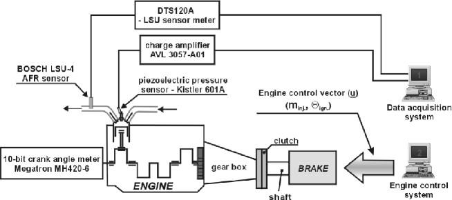
Figure 1: Schematic diagram of the experimental stand for pressure measurements.

In our experimental stand (Fig. 1), the pressure inside the cylinder is measured by a standard method using a piezo-electric sensor. It should be noted that pressure is the best known quantity that can be directly measured to analyze engine dynamics [5, 8, 26, 27, 28, 29]. Actual cylinder pressure together with the internal cylinder volume can be used to obtain the indicated mean effective pressure (IMEP), to calculate the engine torque and efficiency, and also to estimate the magnitudes of important process variables such as burning rate, bulk temperature and heat release. Furthermore, statistical analysis of internal pressure data can provide information about the stability of the combustion process.

Our equipment provides a direct measure of the pressure inside the cylinder of a spark ignition engine. Internal pressure data were recorded at the Engine Laboratory of the Technical University of Lublin, where we conducted a series of tests. The pressure traces were generated on a 1998 cm³ Holden 2.0 MPFI engine running at 1000 revolutions per minute. Measurements were made with a resolution of about $0.7^{o}$ of crankshaft revolution. A single experiment consisted of about 2000 cycles of engine work. Data were collected at different spark timings with spark advance angles of 5, 15 and 30 degrees before the top dead center (TDC). The engine speed, fuel-air ratio, and throttle setting were all held constant throughout the data collection period. Intake air pressure was maintained at 40 kPa and a stoichiometric mixture was used.

A few examples of the pressure measurements are presented in Fig. 2. Here we have plotted the variation of pressure with crank angle during the first 20 combustion cycles for three different values of the spark advance angles: $\Delta\alpha_{z}=5^{o}$, 15^o and 30^o. Note that the pressure measurements reflect the combined effects of cylinder volume compression and combustion of the fuel-air mixture. From these measurements the values of maximum pressure $p_{max}$ and the peak pressure angle $\alpha_{pmax}$ can be easily identified.

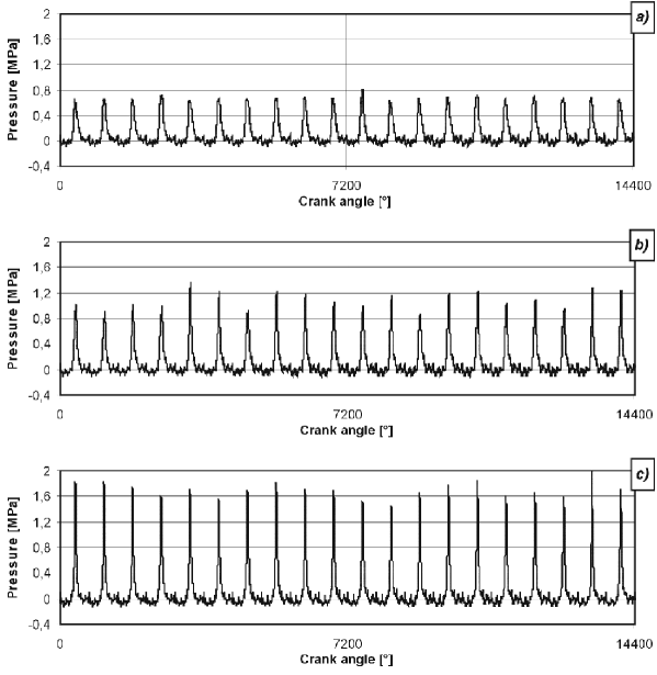
Figure 2: Variations of internal pressure with crank angle during the first 20 combustion cycles. The panels (a), (b) and (c) correspond to the spark advance angles $\Delta\alpha_{z}=5^{o}$, 15^o and 30^o, respectively.

Before we go into a detailed analysis of the time series of $p_{max}$ and $\alpha_{pmax}$ in consecutive combustion cycles, we would like to point out the importance of these quantities for combustion control and diagnostics. Note that the output torque usually scales as the square of the mean values of $p_{max}$ or $\alpha_{pmax}$ for different speeds [7, 24, 25].

3 Cyclic Time Series and Pressure Fluctuations

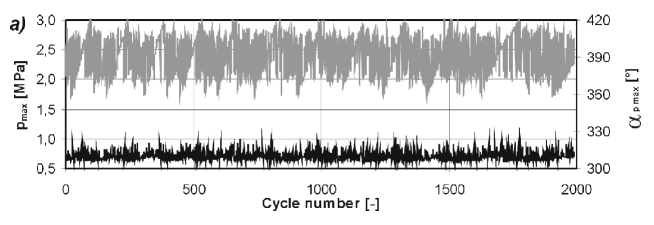
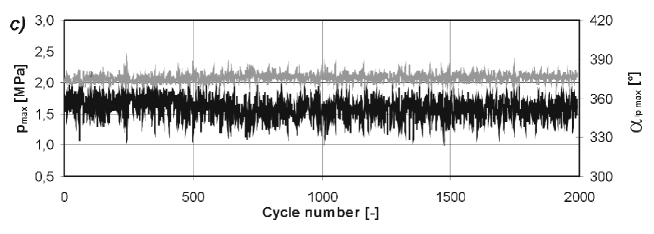
Figure 3: Time series of cycle-to-cycle variations of maximum pressure $p_{max}$ (in black) and $\alpha_{pmax}$ (in grey) for three values of the spark advance angle: $\Delta\alpha_{z}=5^{o}$, 15^o and 30^o, for Figs. 3a-c, respectively.

From Fig. 2 we observe that the cycle-to-cycle fluctuations of pressure are present in all cases considered and they change with the spark advance angle $\Delta\alpha_{z}$. It should be noted that the magnitude of peak pressure, which is directly related to the power output, depends on $\Delta\alpha_{z}$; $p_{max}$ is higher for larger $\Delta\alpha_{z}$. Unfortunately, the advantage of maximum pressure increase is offset by the disadvantage of increasing fluctuations. In terms of the peak pressure $p_{max}$, this effect can be observed in Figs. 3a-c. Here we have also plotted the time series of the corresponding angles $\alpha_{pmax}$ for which the peak pressure $p_{max}$ is reached. Surprisingly, changes in combustion conditions which lead to increased fluctuations of $p_{max}$ are associated with decreased fluctuations of $\alpha_{pmax}$.

3.1 Return Maps

To explore the properties of the time series of $p_{max}$ and $\alpha_{pmax}$ in more detail, we have plotted their return maps for the various spark advance angles. These are shown in Fig. 4. We define a sequential transformation for any cycle $i$:

$$F(i)\rightarrow F(i+1),$$ (1)

 

 

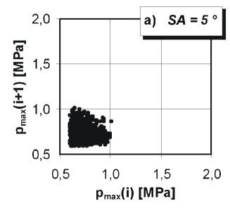
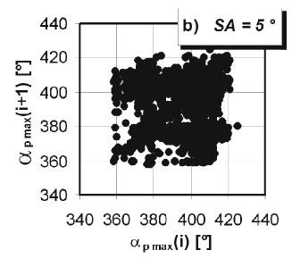
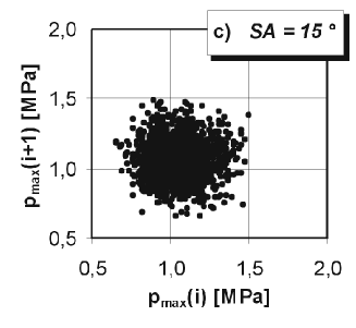
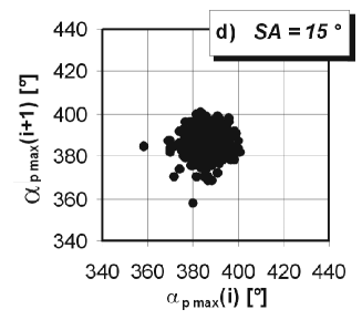
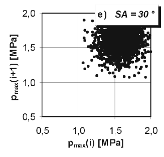
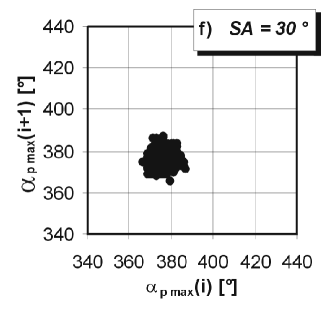
Figure 4: Return maps of cyclic pressure maxima $p_{max}$ and the corresponding angles $\alpha_{pmax}$ for three spark advance angles $\Delta\alpha_{z}$ denoted by SA$=5^{o}$, 15^o and 30^o.

where $F$ can be identified with $p_{max}$ or $\alpha_{pmax}$. In a return map, black points in the coordinates ($F(i+1)$,$F(i)$) are marked. Such maps are very useful in examining changes of the corresponding quantity $F(i)$. The method of return maps has become a standard tool in the investigation of engine dynamics but they are usually applied to burned mass ratio or heat release per cycle [20, 22, 30]. Let us analyze the first diagram (Fig. 4a) which corresponds to the pressure history in Fig. 2a ($\Delta\alpha_{z}=5^{o}$). The characteristic black right angle in the left bottom corner of the return map indicates a very low level of combustion or misfire instabilities. The corner point represents the lowest value of $p_{max}$ which can be identified as peak compression pressure. In terms of peak pressure angles $\alpha_{pmax}$ (Fig. 4b) we observe that the points lying at the lowest angular position around 360^o (for $\Delta\alpha_{z}=5^{o}$) correspond to a maximum compression point – the Top Dead Point (TPD). However, in this case ($\Delta\alpha_{z}=5^{o}$) we cannot draw any conclusion about misfires because we are not analyzing heat release here. Extended studies of this effect can be found in [22, 10, 30, 32]. In Figs. 4c,d and Figs. 4e,f, we show the return maps for the spark advance angles $\Delta\alpha_{z}=15^{o}$ and $30^{o}$, respectively. In these cases the fluctuations may have a different origin. Following the previous analysis for $\Delta\alpha_{z}=15^{o}$ (Figs. 4c,d), we have detected a singular point with relatively weak combustion, while for $\Delta\alpha_{z}=30^{o}$ such points have disappeared. This means that the identification of pressure peak caused by combustion is certain in that regime. Of course, the measured fluctuations will change with changes in the spark advance angle $\Delta\alpha_{z}$ [29]. Statistical features covered by the return maps are in agreement with the time series histories depicted in Fig. 3a-c. Note that the fluctuations in $p_{max}$ increase while those in $\alpha_{pmax}$ decrease with increasing $\Delta\alpha_{z}$. We should also mention that all the maps possesses the approximate diagonal ($F(i+1)$ versus $F(i)$) symmetry; this can be interpreted as the time reversal symmetry of the corresponding time series of $p_{max}$ and $\alpha_{pmax}$. This symmetry has not been broken in contrast to other reports on combustion experiments (Green at al. [22]). The main difference is that Green at al. [22] examined the lean combustion limit whereas our fuel-air mixture is stoichiometric. Clearly, preserved time-reversal symmetry may appear if the stochastic component is significant. Alternatively, for deterministic but chaotic time series one usually observes asymmetry in the return maps [22] associated with a broken time-reversal symmetry.

3.2 Histograms

 

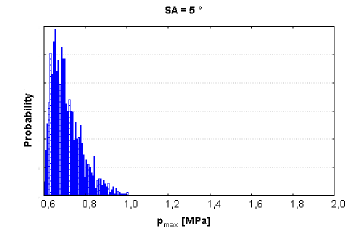
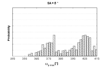
(a)                                                      (b)

 

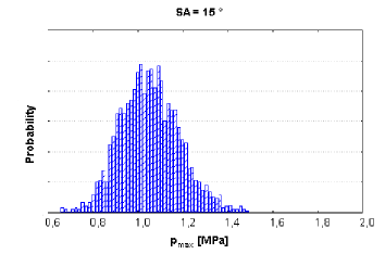
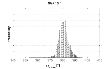
(c)                                                      (d)

 

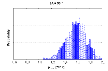
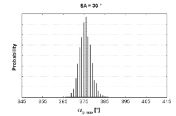
(e)                                                      (f)

Figure 5: Histograms of cyclic pressure maxima $p_{max}$ and the corresponding angles $\alpha_{pmax}$ ($SA=\Delta\alpha_{z}=5^{o},~{}15^{o},~{}30^{o}$).

Here we perform further analysis of the $p_{max}$ and $\alpha_{pmax}$ time series using histograms. From the time series we calculate the probability $P_{n}$:

$$P_{n}=\frac{1}{N_{total}}\sum_{i}^{N_{total}}\Theta(\tilde{F}_{n}-F(i))\Theta(F(i)-\tilde{F}_{n+1}),$$ (2)

where $\Theta(x)$ is the Heaviside step function, $F(i)$ is a sequentially measured quantity, and $\tilde{F}_{n}$ denotes a discretized value. Here $N_{total}=1991$ is the total number of combustion cycles in a single time series. In Figs. 5a-f we have plotted the histograms of the time series for $p_{max}$ or $\alpha_{pmax}$ for the various cases considered in Figs. 4a-f. Interestingly, the combustion process represented by the histograms in Figs. 5a and b can be identified as a process with an ambiguous position of maximum. This effect was also found in the paper by Litak et al. [29]. In fact the double peak structure is clearly visible in Fig. 5b. They are directly related to compression and combustion phenomena. Note that the exponential distribution in Fig. 5a indicates that the measurement process is not continuous, similar to the situation in a cutting process with additional cracking effects [31]. In our case, identification of the pressure peak is not certain because from time to time, especially for weak combustion it is interchanged with compression. On the basis of our experimental data we cannot entirely exclude the possibility of misfires [32]. In Figs. 5c-d and Figs. 5e-f, we show the distributions of $p_{max}$ and $\alpha_{pmax}$ for $\Delta\alpha_{z}=15^{o}$ and $\Delta\alpha_{z}=30^{o}$, respectively. Comparing these figures with Figs. 5a-b, we see that they are substantially different having more or less the Gaussian shape with small asymmetry. Again we observe a characteristic broadening in $p_{max}$ and a narrowing in $\alpha_{pmax}$with increasing $\Delta\alpha_{z}$ .

3.3 Multiscale Entropy

Many physical systems evolve on multiple temporal and/or spatial scales and are governed by complex dynamics. In recent years there has been a great deal of interest in quantifying the complexity of these systems. However, no clear and unambiguous definition of complexity has been established in the literature. Intuitively, complexity is associated with ”meaningful structural richness” [34]. Several notions of entropy have been introduced to describe complexity in a more precise way. But, as Costa et al. [35] have pointed out, these traditional entropy measures quantify the regularity (predictability) of the underlying time series on a single scale, and there is no direct correspondence between regularity and complexity. For instance, neither completely predictable (e.g., periodic) signals, which have minimum entropy, nor completely unpredictable (e.g., uncorrelated random) signals, which have maximum entropy, are truly complex. For complex systems with multiple temporal or spatial scales, a definition of complexity should include these multiscale features. Recently Costa et al. [35] introduced the concept of multiscale entropy (MSE) to describe the complexity of such multiscale systems. They have successfully used this concept to describe the nature of complexity in physiological time series such as those associated with cardiac dynamics [37] and gait mechanics [36]. In this paper we perform a multiscale entropy analysis as a measure of complexity in cycle-to-cycle variations of maximum pressure and peak pressure angle in a spark ignition engine. MSE is based on a coarse-graining procedure and can be carried out on a time series as follows.

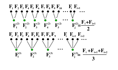
Figure 6: Schematic diagram of the coarse-graining procedure used in the calculation of multiscale sample entropy (after [34]). Note, $F^{(1)}_{i}=F_{i}$ and $\tau$ is the scale factor.

For a given time series $\{F_{1},F_{2},...,F_{n}\}$, where $F_{i}=F(i)$, multiple coarse-grained time series are constructed by averaging the data points within non-overlapping windows of increasing length as shown in Fig. 6. Each element of the coarse-grained time series is computed according to the equation:

$$F_{j}^{(\tau)}=\frac{1}{\tau}\sum_{i=(j-1)\tau+1}^{j\tau}F_{i}.$$ (3)

Here $\tau$ represents the scale factor, and $1\leq j\leq N/\tau$, the length of each coarse-grained time series being equal to $N/\tau$. Note that for $\tau=1$, the coarse-grained time series is simply the original time series.

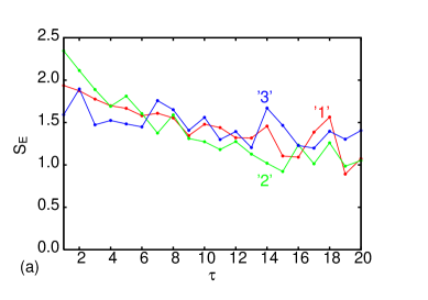
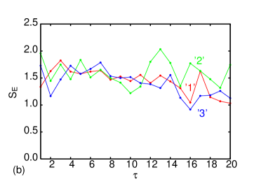
Figure 7: Sample entropy $S_{E}$ calculated for normalized time series $F_{i}=p_{max}(i)/\sigma_{(}p_{max})$ (a) and $\alpha_{pmax}/\sigma(\alpha{pmax})$ (b) versus the scale factor $\tau$. $\sigma(p_{max})$ and $\sigma(\alpha_{pmax})$ denote square root deviations of $p_{max}$ and $\alpha_{pmax}$, respectively. The length of chain $m=3$ and similarity factor $r=0.15$ for all time series. Curves ’1’, ’2’ and ’3’ correspond to $\Delta\alpha_{z}=5^{o}$, 15^o and 30^o, respectively.

The sample entropy $S_{E}$, proposed originally by Richman and Moorman [38] is calculated for the sequence of $m$ consecutive data points which are ’similar’ to each other and will remain similar when one or more consecutive data points are included [38]. Here ’similar’ means that the value of a specific measure of distance is less than a prescribed amount $r$. Therefore, the sample entropy depends on two parameters $m$ and $r$. We have

$$S_{E}(m,r,N)=\ln\frac{\sum_{i=1}^{N-m}\{\tilde{F}(i,m,r)\}}{\sum_{i=1}^{N-m-1}\{\tilde{F}(i,m+1,r)\}}$$ (4)

The sample entropy has been calculated for each of the coarse-grained time series of $p_{max}$ and $\alpha_{pmax}$ and then plotted as a function of the scale factor $(\tau)$. The results are shown in Fig. 7, where Fig. 7a corresponds to $p_{max}$ and Fig. 7b to $\alpha_{pmax}$. It should be noted that for a simple but stochastic system the sample entropy $S_{E}$ has a hyperbolic shape. This shape can be identified only for curve ’2’ in Fig. 7a while the curves ’1’ and ’3’ are definitely more flat. In Fig. 7b, on the other hand, all curves have a mild dependence on $\tau$, and can be described approximately by horizontal lines. Such horizontal lines are typical for strongly asymmetric distributions such as 1/f noise. In fact, if one looks more carefully at the slopes of the histograms of our signals, one can notice the obvious asymmetry in Figs. 5b and e, and to some extent in Figs. 5d,f. Note that the peculiar nonlinear dynamics and a limited length of time series can additionally disturb these characteristics and produce fluctuations along the $\tau$ axis (Fig. 7). Interestingly the results show that $p_{max}$ and $\alpha_{pmax}$ are characterized by quite different aspects of the same dynamical process.

4 Discussion and Conclusions

We have used the maximum pressure $p_{max}$ and the peak pressure angle $\alpha_{pmax}$ as variables for describing the combustion process in a spark ignition engine. Their cycle-to-cycle variations are analyzed using different techniques such as return maps, histograms and multiscale entropy. Until now, researchers have used only one of these variables to formulate an objective function for optimization and control of engine dynamics. Prompted by these complementary analyses of $p_{max}$ and $\alpha_{pmax}$ presented in the literature [29, 33, 24], we propose to use a mutual criterion for combustion efficiency in the SI engine. Instead of minimizing the fluctuations of $p_{max}$ or $\alpha_{pmax}$ by looking at their smallest standard deviation $\sigma(p_{max})$, or $\sigma(\alpha_{pmax})$:

$$(a)~{}~{}~{}~{}~{}~{} \sigma(p_{max})=\frac{1}{\delta p_{max}}\sqrt{\frac{1}{N_{total}}\sum_{i=1}^{N_{total}}\left(p_{max}(i)-\overline{p_{max}}\right)^{2}}$$

$$(b)~{}~{}~{}~{}~{}~{} \sigma(\alpha_{pmax})=\frac{1}{\delta\alpha_{pmax}}\sqrt{\frac{1}{N_{total}}\sum_{i=1}^{N_{total}}\left(\alpha_{pmax}(i)-\overline{\alpha_{pmax}}\right)^{2}}$$

we look for a two-variable square deviation $\sigma(p_{max},\alpha_{pmax})$ given by.

$$(c)~{}~{}~{}~{}~{}~{} \sigma(p_{max},\alpha_{pmax})=$$ (6)

$$\sqrt{\frac{1}{N_{total}}\sum_{i=1}^{N_{total}}\left(\frac{\left(p_{max}(i)-\overline{p_{max}}\right)^{2}}{(\delta p_{max})^{2}}+\frac{\left(\alpha_{pmax}(i)-\overline{\alpha_{pmax}}\right)^{2}}{(\delta\alpha_{pmax})^{2}}\right)},$$

where $\delta p_{max}$ and $\delta\alpha_{pmax}$ are chosen as the largest of $\sigma_{pmax}$ and $\sigma(\alpha_{pmax})$ from all examined cases and are treated as normalization.

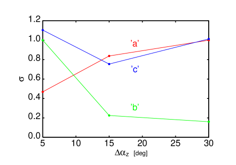
Figure 8: Square deviations $\sigma p_{max}$ (a), $\sigma(\alpha_{pmax})$ (b) and $\sigma(p_{max},\alpha_{pmax})$ (c) as a generalized efficiency criterion (notation (a)-(c) as in Eqs. 4-6).

All the above square deviations are plotted in Fig. 8. In this figure note that the plot for $\sigma(p_{max},\alpha_{pmax})$ has a minimum when $\Delta\alpha_{z}=15^{o}$. In our previous paper[13], where we analyzed noise effects in the cycle-to-cycle fluctuations of heat release, we noticed that $\Delta\alpha_{z}=15^{o}$ is the case of optimal combustion conditions. Now we see that for $\Delta\alpha_{z}=30^{o}$ the oscillations of $p_{max}$ are the largest. On the other hand, for $\Delta\alpha_{z}=5^{o}$ the fluctuations in $\sigma(\alpha_{pmax})$ are significant. The average heat release which varies with the spark advance angle has magnitudes of 352.54J for $\Delta\alpha_{z}=5^{o}$, 396.67J for $\Delta\alpha_{z}=15^{o}$ and 377.04J for $\Delta\alpha_{z}=30^{o}$ [13]. It is the largest for $\Delta\alpha_{z}=15^{o}$ indicating the largest burning rate of fuel while the output torque, for the same speed of the crankshaft, is changing from the largest value: $S=30$Nm, in the case of $\Delta\alpha_{z}=30^{o}$, to a slightly smaller value: $S=28$Nm for $\Delta\alpha_{z}=15^{o}$, and to an even smaller value: $S=21$Nm for $\Delta\alpha_{z}=5^{o}$. Knowing that the fresh fuel rate was the same in all the cases, we concluded that there were better combustion conditions for larger spark advance angles. Additionally, in case of $\Delta\alpha_{z}=5^{o}$ some amount of fuel was not burned because of weak combustion or misfires. In the previous paper [13] our analysis of noise level led us to the conclusion that in the case of $\Delta\alpha_{z}=15^{o}$, the combustion process was most stable.

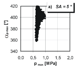
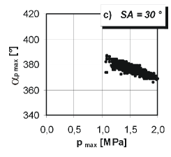
(a)                                   (b)                                   (c)

Figure 9: Maximum pressure-angle diagrams ($p_{max}$, $\alpha_{pmax}$) for three advance angles ($SA=\Delta\alpha_{z}=5^{o}$ (a), $15^{o}$ (b), $30^{o}$ (c)).

Here we have found another argument leading to the same conclusion based on the two variables $p_{max}$ and $\alpha_{pmax}$. Furthermore, from the multiscale entropy analysis we find that the $p_{max}$ sequence is governed by the simplest dynamics. Examining both $[p_{max},\alpha_{pmax}]$ time series simultaneously it becomes clear that the two variable square deviation $(\sigma(p_{max},\alpha_{pmax}))$ may play an important role in the optimization procedure. In Figs. 9a-c we plotted the variables for each combustion cycle. Following our philosophy, these plots may be called ’a bifurcation diagram’. They show the transition from the case of $\alpha_{pmax}$-dominated fluctuations (Fig. 9a for $\Delta\alpha_{z}=5^{o}$) to the case of $p_{max}$-dominated fluctuations (Fig. 9c for $\Delta\alpha_{z}=30^{o}$) through the intermediate case (Fig. 9b for $\Delta\alpha_{z}=15^{o}$). One can easily see the qualitative change in the fluctuation type starting from a vertical line structure in Fig. 9a and ending with an almost horizontal line in Fig. 9c. It is worth pointing out that both types of fluctuations are harmful for a stable engine operation and may result in decreased power output. It appears that the intermediate case is a compromise between these two types of fluctuations. The detailed analysis of the relations between $p_{max}$ and $\alpha_{pmax}$ can provide further useful information on combustion dynamics as the rate of slow and/or fast individual burning processes during engine use corresponding to slow and fast heat release. The two extreme realizations of a combustion process presented in Fig. 9a and Fig. 9c (for $\Delta\alpha_{z}=5^{o}$ and $30^{o}$, respectively) can be directly related to slow and fast burning [27]. Obviously the fast burning is not so effective as slow burning because it may involve some events corresponding to a spatially limited engine volume. Thus, as expected, if slow burning dominates, then the fluctuations of $p_{max}$ are small (Figs. 9a and 3a), whereas for fast burning the fluctuations of $p_{max}$ are larger (Figs. 9c and 3c). Interestingly, measured fluctuations of $\alpha_{pmax}$ are governed mainly by the ambiguity of identification of maximum pressure and possibly by a misfire phenomenon [32]. These two effects have opposite influences on $p_{max}$ and $\alpha_{pmax}$. On this basis our formulation of optimization procedure (Eq. 6) seems to be a natural consequence of a detailed analysis of the pressure-angle diagrams Figs. 9a-c. The minimum standard deviation defined in the $(p_{max},\alpha_{pmax})$ plane, realized for $\Delta\alpha_{z}=15^{o}$, can be regarded as a compromise between the maximizing of power output and minimizing of pressure fluctuations. Clearly, larger power is accompanied by unstable combustion with larger pressure oscillations.

It is worth noting that our simple mutual criterion seems to unify these approaches. Using this criterion we can associate the optimal combustion conditions with the spark advance angle $\Delta\alpha_{z}=15^{o}$. Of course, for any practical application we would need to consider many more values of $\Delta\alpha_{z}$ and more importantly check the output torque [8].

References

- [1] D. Clerk, The Gas Engine, (Longmans, Green & Co., London 1886).
- [2] D.J. Patterson, Cylinder pressure variations, a fundamental combustion problem, SAE paper No. 660129, 1966.
- [3] M. Hubbard, P.D. Dobson, and J.D. Powell, Closed loop control of spark advance using a cylinder pressure sensor, Journal of Dynamic Systems, Measurement and Control (1976) 414–420.
- [4] F.A. Matekunas, Engine combustion control with ignition timing by pressure ratio management, US Pat., A 4622939 Nov. 18 1986.
- [5] K. Sawamoto, Y. Kawamura, T. Kita and K. Matsushita, Individual cylinder knock control by detecting cylinder pressure. SAE paper No. 871911, 1987.
- [6] R.M. Wagner, C.S. Daw, and J.F Thomas, Controlling chaos in spark-ignition engines. in Proceedings of the Central and Eastern States Joint Technical Meeting of the Combustion Institute (New Orleans, 1993 March 15-17).
- [7] L. Eriksson, L. Nilsen, M. Glavenius, Development of control algorithm stabilizing torque for optimal position of pressure peak, SAE Transactions Journal of Engines 106 (1997) 1216–1223.
- [8] J.B. Heywood, Internal Combustion Engine Fundamentals, McGraw-Hill, New York 1988.
- [9] Z. Hu, Nonlinear instabilities of combustion processes and cycle-to-cycle variations in spark-ignition engines, SAE paper No. 961197, 1996.
- [10] R.M. Wagner, J.A. Drallmeier, and C.S. Daw, Characterization of lean combustion instability in pre-mixed charge spark ignition engines, International Journal of Engine Research 1 (2001) 301–320.
- [11] C.S. Daw, C.E.A. Finney, and E.R. Tracy, A review of symbolic analysis of experimental time series, Rev. of Scen. Instr. 74 ( 2003) 915–930.
- [12] M. Wendeker, J. Czarnigowski, G. Litak, and K. Szabelski, Chaotic combustion in spark ignition engines, Chaos, Solitons & Fractals 18 (2003) 803–806.
- [13] T. Kamiński, M. Wendeker, K. Urbanowicz, and G. Litak, Combustion process in a spark ignition engine: dynamics and noise level estimation, Chaos 14 (2004) 461–466.
- [14] R.E. Winsor and D.J. Patterson, Mixture turbulence – a key to cyclic combustion variation, SAE paper No. 730086, 1973.
- [15] J.W. Daily, ”Cycle-to-cycle variations: a chaotic process?” Combustion Science and Technology 57 (1988) 149–162.
- [16] J.C. Kantor, A dynamical instability of spark-ignited engines”, Science 224 (1984) 1233–1235.
- [17] A.P. Foakes and D.G. Pollard, Investigation of a chaotic mechanism for cycle-to-cycle variations, Combustion Science and Technology 90 (1993) 281–287.
- [18] L. Chew, R. Hoekstra, J.F. Nayfeh, and J. Navedo, Chaos analysis of in-cylinder pressure measurements, SAE paper No. 942486, 1994.
- [19] C. Letellier, S. Meunier-Guttin-Cluzel, G. Gouesbet, F. Neveu, T. Duverger, and B. Cousyn, Use of the nonlinear dynamical system theory to study cycle-to-cycle variations from spark-ignition engine pressure data, SAE paper No. 971640, 1997.
- [20] C.S. Daw, C.E.A. Finney, J.B. Green, Jr., M.B. Kennel, J.F. Thomas, and F.T. Connolly, A simple model for cyclic variations in a spark-ignition engine, SAE paper No. 962086, 1996.
- [21] C.S. Daw, M.B. Kennel, C.E.A. Finney, and F.T. Connolly, Observing and modelling dynamics in an internal combustion engine, Physical Review E 57 (1998) 2811–2819.
- [22] J.B. Green Jr, C.S. Daw, J.S. Armfield, C.E.A. Finney, R.M. Wagner, J.A. Drallmeier, M.B. Kennel, and P. Durbetaki, Time irreversibility and comparison of cyclic-variability models, SAE paper No. 1999-01-0221, 1999.
- [23] M. Wendeker, G. Litak, J. Czarnigowski, and K. Szabelski, Nonperiodic oscillations in a spark ignition engine, Int. J. Bifurcation and Chaos 14 (2004) 1801–1806.
- [24] L. Nielsen and L. Eriksson, An ion-sense engine-fine-tuner, IEEE Control Systems Magazine 18 (1998) 43 -52.
- [25] T. Kaminski, PhD thesis, Technical University of Lublin, Lublin 2005.
- [26] F.A. Matekunas, Modes and measures of cyclic combustion variability, SAE paper No. 830337, 1983.
- [27] N. Ozdor, M. Dulger, and E. Sher, Cyclic variability in spark ignition engines: a literature survey, SAE paper No. paper 940987, 1994.
- [28] R. Radu and R. Taccani, Experimental setup for the cyclic variability analysis on a spark ignition engine, SAE NA paper No. 2003-01-19 (2003).
- [29] G. Litak, R. Taccani, R. Radu, K. Urbanowicz, M. Wendeker, J.A. Hołyst, and A. Giadrossi, Estimation of the noise level using coarse-grained entropy of experimental time series of internal pressure in a combustion engine, Chaos, Solitons & Fractals, 23 (2005) 1695-1701.
- [30] G. Litak, M. Wendeker, M. Krupa, and J. Czarnigowski, A numerical study of a simple stochastic/ deterministic model of cycle-to-cycle combustion fluctuations in spark ignition engines, Journal of Vibration and Control 11 (2005) 371-379.
- [31] G. Radons, R. Neugebauer (Eds.) Nonlinear Dynamic Effects of Production Systems, (Wiley-VCH, Weinheim 2004).
- [32] D. Piernikarski and J. Hunicz, Investigation of misfire nature using optical combustion sensor in a SI automotive engine, SAE paper No. 2000-02-0549 (2000).
- [33] L. Eriksson, Spark advance for optimal efficiency, SAE paper No. 99-01-0548, 1999.
- [34] P. Grassberger, in Information Dynamics, (Eds.) H. Atmanspacher and H. Scheingraber, (Plenum Press, New York 1991).
- [35] M. Costa, A. L. Goldberger, C.-K. Peng, Multiscale analysis of complex biological signals, Phys. Rev. Lett. 89, (2002) 068102.
- [36] M. Costa, C.-K. Peng, A. L. Goldberger, Multiscale analysis of human gait dynamics, Physica A 330 (2003) 53-60.
- [37] M. Costa, A. L. Goldberger, C.-K. Peng, Multiscale analysis of biological signals, Phys. Rev. E 89 (2005) 021906.
- [38] J.S. Richman and J.R. Moorman, Physiological time-series analysis using approximate entropy and sample entropy, Am. J. Physiol 278 (2000) H2039-H2049.