Magnetic field gradients in solar wind plasma and geophysics periods

Abstract

Using recent data obtained by Advanced Composition Explorer (ACE) the pumping scale of the magnetic field gradients of the solar wind plasma has been calculated. This pumping scale is found to be equal to 24h $\pm$ 2h. The ACE spacecraft orbits at the L1 libration point which is a point of Earth-Sun gravitational equilibrium about 1.5 million km from Earth. Since the Earth’s magnetosphere extends into the vacuum of space from approximately 80 to 60,000 kilometers on the side toward the Sun the pumping scale cannot be a consequence of the 24h-period of the Earth’s rotation. Vise versa, a speculation is suggested that for the very long time of the coexistence of Earth and of the solar wind the weak interaction between the solar wind and Earth could lead to stochastic synchronization between the Earth’s rotation and the pumping scale of the solar wind magnetic field gradients. This synchronization could transform an original period of the Earth’s rotation to the period close to the pumping scale of the solar wind magnetic field gradients.

I Introduction

Magnetic field in solar wind plasma is actively studied in the last years both theoretically and experimentally (see, for instance, barn1 -zmd ). Properties of this field gradients are of especial interest because of strong non-homogeneity of the field. Inferring universal properties of the magnetic field is a difficult task due to superposition of the strong non-homogeneity and global anisotropy. Even in the inertial range of scales the non-homogeneity and anisotropy affect behavior of different components of the magnetic field and its gradients. It can be shown bs , however, that magnitude of the magnetic field $B=\sqrt{B_{i}^{2}}$ does exhibit certain universal properties in inertial range of scales. Moreover, we will show in present paper that magnitude of gradients of the solar wind magnetic field exhibits certain universal properties as well. These universal properties have substantial geophysical consequences, which we discuss in the last section of the paper.

In magnetohydrodynamics (MHD) the magnetic field fluctuation ${\bf B}$ dynamics is described by equation

$$\frac{\partial{\bf B}}{\partial t}=\nabla\times({\bf v}\times{\bf B})+\eta\nabla^{2}{\bf B}.$$

Here, ${\bf v}$ is the turbulence velocity and the $\eta$ is magnetic diffusivity. Equation (1) can be regarded as a vector analogue of the advection-diffusion equation

$$\frac{\partial\theta}{\partial t}=-({\bf v}\cdot\nabla)\theta+D\nabla^{2}\theta$$

for the evolution of a passive scalar $\theta$ subject to molecular diffusivity $D$. Aside from the fact that ${\bf B}$ is a vector and $\theta$ a scalar, the equations are different also because $\bf v$ in Eq. (1) can be affected quite readily by the feedback of the magnetic field $\bf B$. Our interest here is to explore the extent of similarities, despite these obvious differences, in the inertial (Batchelor) range statistics of the magnetic and the passive scalar fields (see, for instance, Refs. shr -ching and the papers cited there).

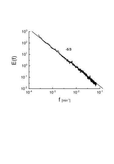
Figure 1: Energy spectrum of the magnitude $B=\sqrt{B_{i}^{2}}$ of the magnetic field $\bf B$ in the solar wind plasma, as measured by the ACE magnetometers in the nanoTesla range for the year 1998 (4 min average).

Solar wind is an excellent natural “laboratory” for the MHD problem. It is known that the statistical properties of velocity fluctuations in the solar wind are remarkably similar to those observed in fluid turbulence bur . It is also known that the plasma power spectra of the magnetic field and velocity fluctuations often contain an “inertial” range with a slope of approximately $-5/3$ (for reviews, see bur ,gold ). The approximately $-5/3$ power-law is especially common for magnitude fluctuations $B=\sqrt{B_{i}^{2}}$ (the summation over repeated indexes is assumed) of the magnetic field, as one can see in Fig. 1. For computing this spectrum, we have used the data obtained from Advanced Composition Explorer (ACE) satellite magnetometers for the year 1998. In this period, the sun was quiet and the data are statistically stable. The range of scales for which the “$-5/3$” power holds is taken to be the inertial range; the smaller scales are obliterated because of the instrument resolution and the truncation at the large-scale end is governed by the record length chosen for Fourier transforming.

The nature of the spectrum for each individual component of the magnetic field is more variable from one component of $\bf B$ to another, and from one situation to another, perhaps because of large anisotropies in the magnetic field $\bf B$, but the result for the $magnitude$ of $\bf B$ seems more robust. Scaling spectrum with the $-5/3$ slope (Fig. 1) is quite typical of that observed for passive scalar fluctuations in fully developed three-dimensional fluid turbulence (the so-called Corrsin-Obukhov spectrum my ). Spurred by this similarity, we were motivated to explore further the properties of the magnitude $B$ and its gradients, and compare them with those of the passive scalar.

II Statistical properties of the magnitude of the magnetic field

More detailed statistical information is provided by the structure functions scaling

$$\langle|\Delta B_{\tau}|^{p}\rangle\sim\tau^{\zeta_{p}},$$

where

$$\Delta B_{\tau}=B(t+\tau)-B(t).$$

The exponent $\zeta_{2}$ is directly related to the spectral exponent (in our case $\zeta_{2}\approx 5/3-1=2/3$ my ). If the dependence of $\zeta_{p}$ on $p$ is nonlinear, it is well-known that one has to deal with intermittency.

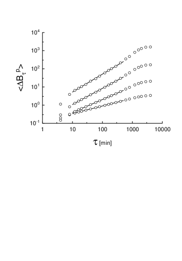
Figure 2: Structure functions of magnetic field magnitude in the solar wind plasma as measured by the ACE magnetometers in nanoTesla for the year 1998 (4 min averages). The straight lines (the best fits) are drawn to indicate the scaling law (3) in the inertial range.

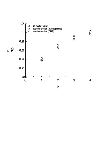
Figure 3: Scaling exponents (3) calculated for $B$ in the solar wind (circles) and for the passive scalar in the atmospheric turbulence (triangles, schmidt ), and in the direct numerical simulation of 3D fluid turbulence (stars, gotoh )

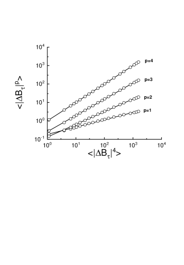
Figure 4: Extended self-similarity (ESS) of the magnetic field magnitude in the solar wind plasma. The straight lines (the best fit) are drawn to indicate the ESS (6).

Figure 5: The same as in Fig. 3 but using the ESS method (6) for $B$.

Figure 2 shows the scaling of structure functions for the solar wind data. Slopes of the straight-line fits in the apparently scaling region provide us the scaling exponents $\zeta_{p}$; these are shown in Fig. 3 as circles. Triangles in the figure indicate experimental values obtained for temperature fluctuations in the atmosphere schmidt . The other experimental data other1 ,other2 are in agreement with each other to better than 5$\%$. The $\star$ symbols are for the passive scalar field obtained by numerically solving the advection-diffusion in three-dimensional turbulence gotoh . It is clear that the exponents for the passive scalar data are in essential agreement with those for the magnitude fluctuations of the magnetic field.

One can, in fact, analyze the solar wind data somewhat differently using the notion of the extended self-similarity (ESS). Since, empirically, the fourth order exponent is quite closely equal to 1 for the magnetic field magnitude, i.e.,

$$\langle|\Delta B_{\tau}|^{4}\rangle\sim\tau,$$

we can extend the scaling range (and consequently improve the confidence with which those exponents are determined) by redefining them as

$$\langle|\Delta B_{\tau}|^{p}\rangle\sim\langle|\Delta B_{\tau}|^{4}\rangle^{\zeta_{p}}.$$

Figure 4 shows the ESS dependence (6). The slopes of the best-fit straight lines in this figure provide us with the ESS scaling exponents $\zeta_{p}$, which are shown in Fig. 5 as circles. The other symbols have remained unchanged from Fig. 3. The shift of the exponents $\zeta_{p}$ in comparison to those from ordinary self-similarity is about 4$\%$, but the scaling interval for ESS is considerably larger. This increased scaling range is well-known in other contexts ben .

The results shown in Figs. 3 and 5 suggest that at least up to the level of the fourth-order the scaling exponents for the passive scalars and for the magnitude of the magnetic field are essentially the same. This is both surprising and thought-provoking, and needs to be understood further. To this end, let us return to Eq. (1) and specialize comment , for simplicity, to the case of incompressible moving medium ($\nabla\cdot{\bf v}=0$). Equation (1) can then be rewritten as

$$\frac{\partial{\bf B}}{\partial t}=-({\bf v}\cdot\nabla){\bf B}+({\bf B}\cdot\nabla){\bf v}+\eta\nabla^{2}{\bf B}.$$

Let us now consider the equation for the magnitude $B$ of the magnetic fluctuations given by ${\bf B}=B{\bf n}$, where ${\bf n}$ is the unit vector with its direction along ${\bf B}$: $n_{i}=B_{i}/B$. Multiplying both sides of Eq. (7) by the vector ${\bf n}$ and taking into account that $n_{i}^{2}=1$ we obtain

$$\frac{\partial B}{\partial t}=-({\bf v}\cdot\nabla)B+\eta\nabla^{2}B+\lambda B,$$

in which the “friction-stretching” (or the production) coefficient $\lambda$ in the last term has the form

$$\lambda=n_{i}n_{j}\frac{\partial v_{i}}{\partial x_{j}}-\eta\left(\frac{\partial n_{i}}{\partial x_{j}}\right)^{2},$$

with the indexes $i$ and $j$ representing the space coordinates, and the summation over repeated indexes is assumed. The first term on the right hand side of Eq. (9) is crucial for any dynamo effect.

If the statistical behaviors of $\theta$ and $B$ are to be similar, as suggested by Figs. 1, 3 and 5, we should be able to observe the underlying similarity between Eqs. (2) and (8). There is a major difference corresponding the presence in Eq. (8) of the production term $\lambda B$. However, given the empirical indications that $B$ and $\theta$ are similar in the inertial range, it is appropriate to look for circumstances under which the $\lambda$ term in Eq. (8) may be small. The second term in $\lambda$ is assured to be small because the smallness of the magnetic diffusivity $\eta$, but difficulties may arise from the first term on the right hand side of Eq. (9).

To eliminate directional dependencies in Eq. (8), let us make the following conditional average of that equation. That is, fix the magnitude $B$ in the vector field ${\bf B}=B{\bf n}$ while performing the average over all realizations of the direction vector field ${\bf n}$ permitted by the vector equation (7). Let us denote this ensemble average as $\langle...\rangle_{{\bf n}}$. From the definition, this averaging procedure does not affect $B$ itself, but affects the velocity field ${\bf v}$ and the “friction-stretching” coefficient $\lambda$ in Eq. (8). We thus obtain

$$\frac{\partial B}{\partial t}=-(\langle{\bf v}\rangle_{{\bf n}}\cdot\nabla)B+\eta\nabla^{2}B+\langle\lambda\rangle_{{\bf n}}B.$$

It is worth emphasizing that the solutions of the original equation (7) satisfy Eqs. (8) and (10), but not all possible formal solutions of the Eqs. (8) and (10) satisfy Eq. (7); similarly, not all formal solutions of Eq. (10) satisfy Eq. (8) while all solutions of Eq. (8) do satisfy Eq. (10). Restricting comments to the relationship between Eqs. (8) and (10), the solutions of the two equations are the same only if the initial conditions are the same and if realizations of $\langle{\bf v}\rangle_{\bf n}$ and of $\langle\lambda\rangle_{\bf n}$, related to these initial conditions by the conditional average procedure, are obtained from solutions applicable to Eq. (8).

Returning now to Eq. (10), the conditionally averaged velocity field $\langle{\bf v}\rangle_{{\bf n}}$ may posses statistical properties that are different from those of the original velocity field ${\bf v}$, and there can be circumstances under which $\langle\lambda\rangle_{{\bf n}}=0$, or small. If so, the similarity between Eqs. (2) and (10) (and, consequently, Eq. (8)) can be the basis for the similarity in statistical properties of their solutions. Therefore, finding conditions under which $\langle\lambda\rangle_{{\bf n}}=0$, or small, seems to be a useful exercise.

It is, however, difficult to guess a priori when $\langle\lambda\rangle_{{\bf n}}$ is negligible, because there is no small parameter for the stretching part of $\lambda$. Therefore, let us consider a generic set of conditions, presumably for the inertial range, which can result in $\langle n_{i}n_{j}\partial v_{i}/\partial x_{j}\rangle_{{\bf n}}=0$. This can be a combination of isotropy, which yields

$$\langle n_{i}n_{j}\rangle_{{\bf n}}=0~{}~{}~{}~{}(i\neq j)$$

and

$$\langle n_{1}^{2}\rangle_{{\bf n}}=\langle n_{2}^{2}\rangle_{{\bf n}}=\langle n_{3}^{2}\rangle_{{\bf n}},$$

and statistical independence

$$\langle n_{i}n_{j}\varphi\rangle_{{\bf n}}=\langle n_{i}n_{j}\rangle_{{\bf n}}\langle\varphi\rangle_{{\bf n}},$$

where $\varphi=\partial v_{k}/\partial x_{l}$ for arbitrary $k$ and $l$.

We should emphasize that the conditional average indicated by $\langle\dots\rangle_{{\bf n}}$ and the global average indicated by $\langle\dots\rangle$ are quite different; because of this, the quantity $B$ in (10) remains a fluctuating variable. To eliminate the stretching part from the conditionally averaged coefficient $\langle\lambda\rangle_{{\bf n}}$—this being critical for explaining the observed similarity in the scaling of structure functions between $B$ and $\theta$—one does not need to satisfy conditions (11) and (12) for all realizations of the magnetic field ${\bf B}$, but only for the subset of realizations that gives the main statistical contribution to the structure functions (3). Let us name this subset of realizations as I. The structure functions (3) depend on the statistical properties of the increments with respect to $\tau$, namely $\Delta B_{\tau}$, belonging to the inertial range of scales. One of the consequences of intermittency is that the statistical properties of the increments are essentially different from those of the field ${\bf B}$ itself. Therefore, the subset I need not generally coincide with the subset G, say, that gives the main statistical contribution to the global average $\langle n_{i}n_{j}\partial v_{k}/\partial x_{l}\rangle$. This means, in particular, that the conditions (11) and (12) can be valid for the inertial interval (i.e. for subset I), while globally (i.e. for subset G) these conditions could well be violated.

We now use conditions (11) and (12) in the presence of the incompressibility condition $\partial v_{i}/\partial x_{i}=0$ and obtain

$$\langle\lambda\rangle_{{\bf n}}=-\eta\langle\left(\frac{\partial n_{i}}{\partial x_{j}}\right)^{2}\rangle_{{\bf n}}.$$

That is, the difference between the passive scalar equation (2) and the conditionally averaged equation (10) for $B$ is reduced to pure “friction” with the friction coefficient given by (13). Equation (10) can then be reduced in Lagrangian variables to

$$\frac{dB}{dt}=\langle\lambda\rangle_{{\bf n}}B,$$

with the “multiplicative noise” $\langle\lambda\rangle_{{\bf n}}$ given by Eq. (13). Weak diffusion of Lagrangian “particles” can be described as their wandering around the deterministic trajectories. Introduction of a weak diffusion is equivalent to introduction of additional averaging in Eq. (14) over random trajectories zeld1 . The small parameter $\eta$ in (13) and (14) will then determine a slow time in comparison with the time scales in the inertial interval and will therefore not affect scaling properties of $B$ in the inertial interval. This explains the similarity of scaling between $B$ and $\theta$.

III The magnetic field gradients

If one can neglect the last term in the right-had side of the equation (10) in the inertial range, then one can readily derive equation for the magnitude gradients ${\bf G}\equiv\nabla B$

$$\frac{\partial G_{i}}{\partial t}=-\langle v_{j}\rangle_{{\bf n}}\frac{\partial G_{i}}{\partial x_{j}}-\frac{\partial\langle v_{j}\rangle_{{\bf n}}}{\partial x_{i}}G_{j}+\eta\frac{\partial^{2}G_{i}}{\partial x_{j}^{2}},$$

The magnitude $G$ of the gradient is determined by ${\bf G}=G{\bf g}$, where ${\bf g}$ is the unit vector with its direction along vector ${\bf G}$. Multiplying both sides of Eq. (15) by $g_{i}$, making summation over $i$, and taking into account of the fact that $g_{i}^{2}=1$, we obtain

$$\frac{\partial G}{\partial t}=-(\langle{\bf v}\rangle_{{\bf n}}\cdot\nabla)G+\eta\nabla^{2}G-\lambda^{\prime}G,$$

which is formally similar to Eq. (2) (cf. Eq. (8)) except for the last term in (16). The coefficient $\lambda^{\prime}$ in this term has the form (cf. Eq. (9))

$$\lambda^{\prime}=g_{i}g_{j}\frac{\partial\langle v_{i}\rangle_{{\bf n}}}{\partial x_{j}}+\eta\left(\frac{\partial g_{i}}{\partial x_{j}}\right)^{2}.$$

One can see remarkable similarity to the situation described in previous section. This similarity suggests applying ensemble conditional average similar to that described above. Fix the magnitude $G$ in the vector field ${\bf G}=G{\bf n}$ while performing the average over all realizations of the direction vector field ${\bf g}$ permitted by equation (15). Let us denote this ensemble average as $\langle...\rangle_{{\bf g}}$. From the definition, this averaging procedure does not affect $G$ itself, but modifies the velocity field $\langle{\bf v}\rangle_{{\bf n}}$, which in turn modifies the coefficient $\lambda^{\prime}$ in Eq. (16). We may write

$$\frac{\partial G}{\partial t}=-(\langle\langle{\bf v}\rangle_{{\bf n}}\rangle_{{\bf g}}\cdot\nabla)G+\eta\nabla^{2}G+\langle\lambda^{\prime}\rangle_{{\bf g}}G.$$

The further analysis can be performed precisely as it has been done above for magnitude of magnetic filed itself. Two main consequences of the directional average: isotropization and smoothing of the velocity field $\langle{\bf v}\rangle_{{\bf n}}$ and the ”nullification” of the production term in the conditionally averaged equations, can have different proportions in these two cases. For the above considered case with magnitude of magnetic field the conditionally averaged (on the directions of the magnetic field) velocity was still enough strongly fluctuating to belong to the inertial range paradigm. It is possible, however, that the conditional average on the directions of the magnitude gradients can smooth the already smoothed velocity field $\langle{\bf v}\rangle_{{\bf n}}$ to a substantially non-fluctuating state. In the last case the essential point is that the twice conditionally averaged velocity $\langle\langle{\bf v}\rangle_{{\bf n}}\rangle_{{\bf g}}$ is smoothed substantially in comparison with ${\bf v}$, while the fluctuation of $G$ itself is still rapid in the diffusion-advection equation (18) (because it remains in tact under the conditional average, by virtue of its definition). Under these typical circumstances, the natural expectation (see, for instance, ynaog and references therein) is that the space autocorrelation function can be characterized by a logarithmic behavior chertkov given by

$$C(r)=\frac{\langle G(r)G(0)\rangle}{\langle G(0)^{2}\rangle}\sim\ln\left(\frac{L}{r}\right),$$

The result owes itself to the pioneering work of Batchelor batc , Batchelor2 who applied this general idea to the viscous-convection range of passive scalar fluctuations with large $Pr$. While the two contexts are quite different, they are the same in the sense that the velocity field is smooth whereas the advected quantity is strongly fluctuating.

For turbulent flows the Taylor hypothesis is generally used to interpret the data. This hypothesis states that the intrinsic time dependence of the magnetic field can be ignored when the turbulence is convected past the probes at nearly constant speed. With this hypothesis, the temporal dynamics should reflect the spatial one b . Equation (19) can be rewritten in the temporal terms ($r\rightarrow\tau$ $L\rightarrow\tau_{0}$)

$$C(\tau)=\frac{\langle G(\tau)G(0)\rangle}{\langle G(0)^{2}\rangle}\sim\ln\left(\frac{\tau_{0}}{\tau}\right).$$

This is seen from Figs. 6 and 7 (in the semi-log scales) to apply quite precisely for the solar wind data (the solid straight line indicates the logarithmic dependence (20)) obtained from Advanced Composition Explorer (ACE) satellite magnetometers for the year 1998 (Fig. 6) and for the year 2004 (Fig. 7).

The so-called pumping scale chertkov $L$ (or $\tau_{0}$) in (19),(20) can be defined from the Figs. 6 and 7 as intersection of the solid straight line with the temporal $\tau$ co-ordinate axis: $\tau_{0}\simeq 24h\pm 2h$.

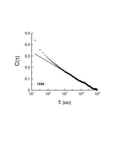
Figure 6: Autocorrelation function $C(\tau)$ of the magnitude of the gradient of $B$ plotted against $\log\tau$, for the ACE-1998 solar wind data.

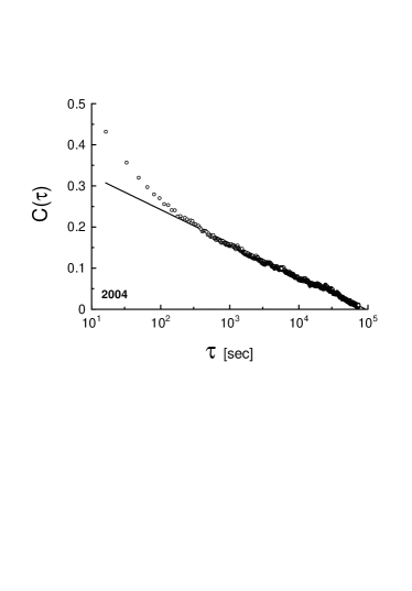
Figure 7: The same as in Fig. 6 but for 2004 year.

IV Geophysical consequences

In order to get away from the effects of the Earth’s magnetic field, the ACE spacecraft orbits at the L1 libration point which is a point of Earth-Sun gravitational equilibrium about 1.5 million km from Earth and 148.5 million km from the Sun. Let us recall that the Earth’s magnetosphere extends into the vacuum of space from approximately 80 to 60,000 kilometers on the side toward the Sun. Therefore, the observed in Figs. 6,7 approximately 24h pumping time-scale of the magnetic field gradients cannot be a consequence of the 24h-period of the Earth’s rotation. The pumping scale certainly corresponds to a process in the solar wind plasma itself. It could be a characteristic scale of the phase coherent structures in the solar wind, which can be distinguished from incoherent fluctuations in this case rg2 (see more about characteristic periods in solar wind plasma in the recent review zmd ). It is now believed that energy of these coherent (pumping) large-scale structures is released via shear instabilities in the solar wind plasma.

It is possible that for the very long time of the coexistence of Earth and of the solar wind the weak interaction between the solar wind and Earth could lead to stochastic synchronization between the Earth’s rotation and the characteristic time-scale (the pumping scale) of the solar wind magnetic field gradients. This synchronization could transform an original period of the Earth’s rotation to the period close to the pumping scale, which we observe at present time.

I thank ACE/MAG instrument team as well as the ACE Science Center for providing the data and support, T. Gotoh for providing Ref. gotoh before publication. I also thank K.R. Sreenivasan for inspiring cooperation, and D. Donzis, J. Schumacher, and V. Steinberg for comments and suggestions.

References

- (1) Barnes A., 1979, Hydrodynamic Waves and Turbulence in the solar Wind, in Solar System Plasma Physics, Vol. I, eds. Parker E.N. Kennel C.F., and Lanzerotti L.J., p. 251, North-Holland.
- (2) Barnes A., 1981, J. Geophy. Res. 86, 7498.
- (3) Belcher J.W. and Davis L. Jr., 1971, J. Geophys. Res., 76, 3534.
- (4) Bershadskii A., 2003, Phys. Rev. Lett., 90, 041101.
- (5) Bershadskii A. and Sreenivasan K.R., 2004, Phys. Rev. Lett., 93, 064501.
- (6) Biskamp D., 1993, Nonlinear Magnetohydrodynamics (Cambridge Univ. Press, Cambridge, UK.).
- (7) Burlaga L.F. and Ness N.F., 1998, J. Geophys. Res., 103, 29719.
- (8) Burlaga L.F., Wang C., Richardson J.D., and Ness N.F., 2003, Ap. J., 585, 1158.
- (9) Goldstein M.L., Burlaga L.F. and Matthaeus, 1984, J . Geophys. Res., 89, 3747.
- (10) Goldstein M.L., 2001, Astrophys. Space Sci. 227, 349.
- (11) Hartlep T., Matthaeus W.H., Padhye N.S., and Smith C.W., (2000), 105, 5135.
- (12) Oughton S., Priest E.R. and Matthaeus W.N., 1994, J. Fluid Mech., 280, 95.
- (13) Roberts D.A. and Goldstein M.L., 1987, J. Geophys. Res., A, 92, 10105.
- (14) Zhou Ye, Matthaeus W.H. and Dmitruk P., 2004, Rev. Mod. Phys., 74, 1015.
- (15) B.I. Shraiman and E.D. Siggia, Nature 405, 639 (2000).
- (16) G. Falkovich, K. Gawedzki and M. Vergassola, Rev. Mod. Phys. 73, 913 (2001).
- (17) Y. Cohen, T. Gilbert and I. Procaccia, Phys. Rev. E 65, 026314 (2002).
- (18) E.S.C. Ching, Y. Cohen, T. Gilbert and I. Procaccia, Phys. Rev. E 67, 016304 (2003).
- (19) L. F. Burlaga, Interplanetary Magnetohydrodynamics (Oxford University Press, New York) 1995.
- (20) M.L. Goldstein, Astrophys. Space Sci. 227, 349 (2001).
- (21) Gotoh T., Fukayama D. & Nakano T., 2002, Phys. Fluids, 14, 1065.
- (22) A.S. Monin and A.M. Yaglom, Statistical Fluid Mechanics: Mechanics of Turbulence, vol. 2 (MIT Press, Cambridge) 1975.
- (23) F. Schmitt, D. Schertzer, S. Lovejoy and Y. Brunet, Europhys. Lett. 34, 195 (1996).
- (24) T. Watanabe and T. Gotoh, Statistics of Passive Scalar in Homogeneous Turbulence (submitted).
- (25) R.A. Antonia, E. Hopfinger, Y. Gagne and F. Anselmet, Phys. Rev. A 30, 2705 (1984).
- (26) C. Meneveau, K.R. Sreenivasan, P. Kailasnath and M.S. Fan, Phys. Rev. A 41, 894 (1990).
- (27) R. Benzi, L. Biferale, S. Ciliberto, M.V. Struglia and R. Tripiccione, Physica D 96, 162 (1996).
- (28) This is not overly restrictive in the inertial range; see, e.g., M.L. Goldstein, D.A. Roberts and W.H. Matthaeus, Annu. Rev. Astron. Astrophys. 33, 283 (1995).
- (29) Ya.B. Zeldovich, A.A. Ruzmaikin and D.D. Sokoloff, Magnetic Fields in Astrophysics (Gordon and Breach) 1983; Ya.B. Zeldovich, B. Molchanov, A.A. Ruzmaikin, D.D. Sokolov Sov. Phys. Usp. 30, 353 (1987).
- (30) Sreenivasan K.R., Bershadskii A., and Niemela J.J., 2005, Phys. Rev. E 71, 035302(R).
- (31) Yuan G.-C., Nam K., Antonsen T.M.. Ott E., and Guzdar P.N., 2000, Chaos 10, 39.
- (32) Chertkov M., Falkovich G., Kolokolov I., and Lebedev V., 1995, Phys. Rev. E 51, 5609.
- (33) Batchelor G.K. , 1959, J. Fluid Mech. 5, 113.
- (34) Batchelor, G.K., 1970, An Introduction to Fluid Dynamics, Cambridge University Press, Cambridge.