Generalized Isothermic Lattices

Abstract.

We study multidimensional quadrilateral lattices satisfying simultaneously two integrable constraints: a quadratic constraint and the projective Moutard constraint. When the lattice is two dimensional and the quadric under consideration is the Möbius sphere one obtains, after the stereographic projection, the discrete isothermic surfaces defined by Bobenko and Pinkall by an algebraic constraint imposed on the (complex) cross-ratio of the circular lattice. We derive the analogous condition for our generalized isthermic lattices using Steiner’s projective structure of conics and we present basic geometric constructions which encode integrability of the lattice. In particular we introduce the Darboux transformation of the generalized isothermic lattice and we derive the corresponding Bianchi permutability principle. Finally, we study two dimensional generalized isothermic lattices, in particular geometry of their initial boundary value problem.

Keywords: discrete geometry; integrable systems; multidimensional quadrilateral lattices; isothermic surfaces; Darboux transformation

1. Introduction

1.1. Isothermic surfaces

In the year 1837 Gabriel Lamé presented [41] results of his studies on distribution of temperature in a homogeneous solid body in thermal equilibrium. He was interested, in particular, in description of the isothermic surfaces, i.e. surfaces of constant temperature within the body; notice that his definition makes sense only for families of surfaces, and not for a single surface. Then he found a condition under which one parameter family of surfaces in (a subset of) ${\mathbb{E}}^{3}$ consists of isothermic surfaces, and showed (for details see [42] or [18]) that the three families of confocal quadrics, which provide elliptic coordinates in ${\mathbb{E}}^{3}$, meet that criterion. Subsequently, he proposed to determine all triply orthogonal systems composed by three isothermic families (triply isothermic systems). Such a program was fulfiled by Gaston Darboux [18] (see also [34]).

Another path of research was initiated by Joseph Bertrand [1] who showed that the surfaces of triply isothermic systems are divided by their lines of curvature into ”infinitesimal squares”, or in exact terms, they allow for conformal curvature parametrization. This definition of isothermic surfaces (or surfaces of isothermic curvature lines), which can be applied to a single surface, was commonly accepted in the second half of the XIX-th century (see [3, 17]). We mention that the minimal surfaces and the constant mean curvature surfaces are particular examples of the isothermic surfaces. The theory of isothermic surfaces was one of the most favorite subjects of study among prominent geometers of that period. Such surfaces exhibit particular properties, for example there exists a transformation, described by Gaston Darboux in [16], which produces from a given isothermic surface a family of new surfaces of the same type.

The Gauss-Mainardi-Codazzi equations for isothermic surfaces constitute a nonlinear system generalizing the $\mathrm{sinh}$-Gordon equation (the latter governs the constant mean curvature surfaces), and the Darboux transformation can be interpreted as Bäcklund-type transformation of the system. Soon after that Luigi Bianchi showed [2] that two Darboux transforms of a given isothermic surface determine in algebraic terms new isothermic surface being their simultaneous Darboux transform. The Bianchi permutability principle can be considered as a hallmark of integrability (in the sense of soliton theory) of the above-mentioned system. Indeed, the isothermic surfaces were reinterpreted by Cieśliński, Goldstein and Sym [12] within the theory of soliton surfaces [53]. More information on isothermic surfaces and their history the Reader can find in the paper of Klimczewski, Nieszporski and Sym [38], where also a more detailed description of the relation between the ”ancient” differential geometry and the soliton theory is given, and in books by Rogers and Schief [48] and by Hertrich-Jeromin [35].

1.2. Discrete isothermic surfaces and discrete integrable geometry

In the recent studies of the relation between geometry and the integrable systems theory a particular attention is payed to discrete (difference) integrable equations and the corresponding discrete surfaces or lattice submanifolds. Also here the discrete analogs of isothermic surfaces played a prominent role in the development of the subject. Bobenko and Pinkall [6] introduced the integrable discrete analogoue of isothermic surfaces as mappings built of ”conformal squares”, i.e., maps ${\boldsymbol{x}}:{\mathbb{Z}}^{2}\to{\mathbb{E}}^{3}$ with all elementary quadrilaterals circular, and such that the complex cross-ratios (with the plane of a quadrilateral identified with the complex plane ${\mathbb{C}}$)

$$q(m,n)=\mathrm{cr}\big{(}{\boldsymbol{x}}(m,n),{\boldsymbol{x}}(m+1,n+1);{\boldsymbol{x}}(m+1,n),{\boldsymbol{x}}(m,n+1)\big{)}_{\mathbb{C}}$$

are equal to $-1$. Soon after that it turned out [7] that it is more convenient to allow for the cross-rations to satisfy the constraint

(1.1) $$q(m,n)q(m+1,n+1)=q(m+1,n)q(m,n+1).$$

Then the cross-ratio is a ratio of functions of single variables, which corresponds to allowed reparametrization of the curvature coordinates on isothermic surfaces.

After the pioneering work of Bobenko and Pinkall, which was an important step in building the geometric approach to integrable discrete equations (see also [25, 5, 19] and older results of the difference geometry (Differenzengeometrie) summarized in Robert Sauer’s books [50, 51]), the discrete isothermic surfaces and their Darboux transformations were studied in a number of papers [36, 11, 52]. Distinguished integrable reductions of isothermic lattices are the discrete constant mean curvature surfaces or the discrete minimal surfaces [7, 35]. It should be mentioned that the complex cross-ratio condition (1.1) was extended to circular lattices of dimension three [7, 11] placing the Darboux transformations of the discrete isothermic surfaces on equal footing with the lattice itself.

In the present-day approach to the relation between discrete integrable systems and geometry [28, 8] the key role is played by the integrable discrete analogue of conjugate nets – multidimensional lattices of planar quadrilaterals (the quadrilateral lattices) [26]. These are maps $x:{\mathbb{Z}}^{N}\to{\mathbb{P}}^{M}$ of $N$-dimensional integer lattice in $M\geq N$-dimensional projective space with all elementary quadrilaterals planar. Integrability of such lattices (for $N>2$) is based on the following elementary geometry fact (see Figure 1).

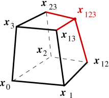
Figure 1. The geometric integrability scheme

Lemma 1 (The geometric integrability scheme).

Consider points $x_{0}$, $x_{1}$, $x_{2}$ and $x_{3}$ in general position in ${\mathbb{P}}^{M}$, $M\geq 3$. On the plane $\langle x_{0},x_{i},x_{j}\rangle$, $1\leq i<j\leq 3$ choose a point $x_{ij}$ not on the lines $\langle x_{0},x_{i}\rangle$, $\langle x_{0},x_{j}\rangle$ and $\langle x_{i},x_{j}\rangle$. Then there exists the unique point $x_{123}$ which belongs simultaneously to the three planes $\langle x_{3},x_{13},x_{23}\rangle$, $\langle x_{2},x_{12},x_{23}\rangle$ and $\langle x_{1},x_{12},x_{13}\rangle$.

Various constraints compatible with the geometric integrability scheme define integrable reductions of the quadrilateral lattice. It turns out that such geometric notion of integrability very often associates integrable reductions of the quadrilateral lattice with classical theorems of incidence geometry. We advocate this point of view in the present paper.

Among basic reductions of the quadrilateral lattice the so called quadratic reductions [20] play a distinguished role. The lattice vertices are then contained in a hyperquadric (or in the intersection of several of them). Such reductions of the quadrilateral lattice can be often associated with various subgeometries of the projective geometry, when the quadric plays the role of the absolute of the geometry (see also corresponding remarks in [20, 21]). In particular, when the hyperquadric is the Möbius hypersphere one obtains, after the stereographic projection, the circular lattices [4, 13, 29, 39], which are the integrable discrete analogue of submanifolds of ${\mathbb{E}}^{M}$ in curvature line parametrization. Because of the Möbius invariance of the complex cross-ratio it is also more convenient to consider (discrete) isothermic surfaces in the Möbius sphere (both dimensions of the lattice and of the sphere can be enlarged) keeping the ”cross-ratio definition”.

For a person trained in the projective geometry it is more or less natural to generalize the Möbius geometry approach to discrete isothermic surfaces (lattices) in quadrics replacing the Möbius sphere by a quadric, and correspondingly, the complex cross-ratio by the Steiner cross-ratio of four points of a conic being intersection of the quadric by the plane of elementary quadrilateral of the quadrilateral lattice. However the ”cross-ratio point of view” doesn’t answer the crucial question about integrability (understood as compatibility of the constraint with the geometric integrablity scheme) of such discrete isothermic surfaces in quadrics. Our general methodological principle in the integrable discrete geometry, applied successfuly earlier, for example in [27, 32], which we would like to follow here is (i) to isolate basic reductions of the quadrilateral lattice and then (ii) to incorporate other geometric systems into the theory considering them as superpositions of the basic reductions.

In this context we would like to recall another equivalent characterization of the classical isothermic surfaces which can be found in the classical monograph of Darboux [17, vol. 2, p. 267]: Les cinq coordonnées pentasphériques d’un point de toute surface isothermique considérées comme fonctions des paramètres $\rho$ et $\rho_{1}$ des lignes de courbure satisfont à une équation linéaire du second ordre dont les invariants sont égaux. Inversement, si une équation de la forme

(1.2) $$\frac{\partial^{2}\theta}{\partial\rho\partial\rho_{1}}=\lambda\theta$$

ou, plus généralement, une équation à invariants égaux, admet cinq solutions particulières $x_{1}$, $x_{2}$, …, $x_{5}$ liées par l’équation

(1.3) $$\sum_{1}^{5}x_{i}^{2}=0,$$

les quantités $x_{i}$ sont les coordonnées pantasphériques qui définissent une surface isothermique rapportée à ses lignes de courbure.

In literature there are known two (closely related) discrete integrable versions (of Nimmo and Schief [46] and of Nieszporski [45]) of the Moutard equation (1.2). It turns out that for our purposes it suits the discrete Moutard equation proposed in [46]. Its projectively invariant geometric characterization has been discovered [33] only recently (for geometric meaning of the adjoint Moutard equation of Nieszporski in terms of the so called Koenigs lattice see [22]). Indeed, it turns out that the generalized isothermic lattices can be obtained by adding to the quadratic constraint the projective Moutard constraint. Finally, the quadratic reduction and the Moutard reduction, when applied simultaneously, give a posteriori the cross-ratio condition (1.1).

In fact, the direct algebraic discrete counterpart of the above description of the isothermic surfaces, i.e. existence of the light-cone lift which satisfies the (discrete) Moutard equation, appeared first in a preprint by Bobenko and Suris [8]. However, the pure geometric characterization of the discrete isothermic surfaces was not given there.

Because integrability of the discrete Moutard equation can be seen better when one considers a system of such equations for multidimensional lattices, there was a need to find the projective geometric characterization of the system. The corresponding reduction of the quadrilateral lattice was called in [23], because of its connection with the discrete BKP equation, the B-quadrilateral lattice (BQL). In fact, research in this direction prevented me from publication of the above mentioned generalization of discrete isothermic surfaces, announced however in my talk during the Workshop ”Geometry and Integrable Systems” (Berlin, 3-7 June 2005). I suggested also there that the discrete S-isothermic surfaces of Tim Hoffmann [37] (see also [8]) should be considered as an example of the generalized isothermic lattices where the quadric under consideration is the Lie quadric. The final results of my research on generalized isothermic lattices were presented on the Conference ”Symmetries and Integrability of Difference Equations VII” (Melbourne, 10-14 July 2006).

When my paper was almost ready there appeared the preprint of Bobenko and Suris [9] where similar ideas were presented in application to the sphere (Möbius, Laguerre and Lie) geometries. I would like also to point out a recent paper by Wallner and Pottman [55] devoted, among others, to discrete isothermic surfaces in the Laguerre geometry.

1.3. Plan of the paper

As it often happens, the logical presentation of results of a research goes in opposite direction to their chronological derivation. In Section 2 we collect some geometric results from the theory of the B-quadrilateral lattices (BQLs) and of quadrilateral lattices in quadrics (QQLs). Some new results concerning the relation between (Steiner’s) cross-ratios of vertices of elementary guadrilaterals of elementary hexahedrons of the QQLs are given there as well. Then in Section 3 we define generalized isothermic lattices and discuss their basic properties. In particular, we give the synthetic-geometry proof of a basic lemma (the half-hexahedron lemma) which immediately gives the cross-ratio characterization of the lattices. We also present some algebraic consequences (some of them known already [8]) of the system of Moutard equations supplemented by a quadratic constraint. In Section 4 we study in more detail the Darboux transformation of the generalized isothermic lattices and the corresponding Bianchi permutability principle. Finally, in Section 5 we consider two dimensional generalized isothermic lattices. In two Appendices we recall necessary information concerning the cross-ratio of four points on a conic curve and we perform some auxilliary calculations.

2. The B-quadrilateral lattices and the quadrilateral lattices in quadrics

It turns out that compatibility of both BQLs and QQLs with the geometric integrablity scheme follows from certain classical geometric facts. We start each section, devoted to a particular lattice, from the corresponding geometric statement.

2.1. The B-quadrilateral lattice [23]

Lemma 2.

Under hypothesess of Lemma 1, assume that the points $x_{0}$, $x_{12}$, $x_{13}$, $x_{23}$ are coplanar, then the points $x_{1}$, $x_{2}$, $x_{3}$, and $x_{123}$ are coplanar as well (see Figure 2).

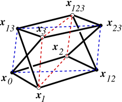
Figure 2. Elementary hexahedron of the B-quadrilateral lattice

As it was discussed in [23] the above fact is equivalent to the Möbius theorem (see, for example [15]) on mutually inscribed tetrahedra. Another equivalent, but more symmetric, formulation of Lemma 2 is provided by the Cox theorem (see [15]): Let $\sigma_{1}$, $\sigma_{2}$, $\sigma_{3}$, $\sigma_{4}$ be four planes of general position through a point $S$. Let $S_{ij}$ be an arbitrary point on the line $\langle\sigma_{i},\sigma_{j}\rangle$. Let $\sigma_{ijk}$ denote the plane $\langle S_{ij},S_{ik},S_{jk}\rangle$. Then the four planes $\sigma_{234}$, $\sigma_{134}$, $\sigma_{124}$, $\sigma_{123}$ all pass through one point $S_{1234}$.

Definition 1.

A quadrilateral lattice $x:{\mathbb{Z}}^{N}\to{\mathbb{P}}^{M}$ is called the B-quadrilateral lattice if for any triple of different indices $i,j,k$ the points $x$, $x_{(ij)}$, $x_{(jk)}$ and $x_{(ik)}$ are coplanar.

Here and in all the paper, given a fuction $F$ on ${\mathbb{Z}}^{N}$, we denote its shift in the $i$th direction in a standard manner: $F_{(i)}(n_{1},\dots,n_{i},\dots,n_{N})=F(n_{1},\dots,n_{i}+1,\dots,n_{N})$. One can show that a quadrilateral lattice $x:{\mathbb{Z}}^{N}\to{\mathbb{P}}^{M}$ is a B-quadrilateral lattice if and only if it allows for a homogoneous representation ${\boldsymbol{x}}:{\mathbb{Z}}^{N}\to{\mathbb{R}}^{M+1}_{*}$ satisfying the system of discrete Moutard equations (the discrete BKP linear problem)

(2.1) $${\boldsymbol{x}}_{(ij)}-{\boldsymbol{x}}=f^{ij}({\boldsymbol{x}}_{(i)}-{\boldsymbol{x}}_{(j)}),\quad 1\leq i<j\leq N,$$

for suitable functions $f^{ij}:{\mathbb{Z}}^{N}\to{\mathbb{R}}$.

The compatibility condition of the system (2.1) implies that the functions $f^{ij}$ can be written in terms of the potential $\tau:{\mathbb{Z}}^{N}\to{\mathbb{R}}$,

(2.2) $$f^{ij}=\frac{\tau_{(i)}\tau_{(j)}}{\tau\,\tau_{(ij)}},\qquad i\neq j,$$

which satisfies Miwa’s discrete BKP equations [44]

(2.3) $$\tau\,\tau_{(ijk)}=\tau_{(ij)}\tau_{(k)}-\tau_{(ik)}\tau_{(j)}+\tau_{(jk)}\tau_{(i)},\quad 1\leq i<j<k\leq N.$$

Remark.

The trapezoidal lattice [8] is another reduction of the quadrilateral lattice being algebraically described by the discrete Moutard equations (2.1). Geometrically, the trapezoidal lattices are characterized by parallelity of diagonals of the elementary quadrilaterals, thus they belong to the affine geometry. Moreover, because the trapezoidal constraint is imposed on the level of elementary quadrilaterals then, from the point of view of the geometric integrability scheme, one has to check its three dimensional consistency. In contrary, the BQL constraint is imposed on the level of elementary hexahedrons, and to prove geometrically its integrability one has to check four dimensional consistency.

2.2. The quadrilateral lattices in quadrics

Lemma 3.

Under hypotheses of Lemma 1, assume that the points $x_{0}$, $x_{1}$, $x_{2}$, $x_{3}$, $x_{12}$, $x_{13}$, $x_{23}$ belong to a quadric $\mathcal{Q}$. Then the point $x_{123}$ belongs to the quadric $\mathcal{Q}$ as well.

Remark.

The above fact is a consequence of the classical eight points theorem (see, for example [15]) which says that seven points in general position determine a unique eighth point, such that every quadric through the seven passes also through the eighth. In our case the point $x_{123}$ is contained in the three (degenerate) quadrics being pairs of opposite facets of the hexahedron.

Remark.

Lemma 2 can be considered as a ”reduced” resion of Lemma 3 when the quadric $\mathcal{Q}$ degenerates to a pair of planes.

Definition 2.

A quadrilateral lattice $x:{\mathbb{Z}}^{N}\to\mathcal{Q}\subset{\mathbb{P}}^{M}$ contained in a hyperquadric $\mathcal{Q}$ is called the $\mathcal{Q}$-reduced quadrilateral lattice (QQL).

Integrability of the QQLs was pointed out in [20], where also the corresponding Darboux-type transformation (called in this context the Ribaucour transformation) was constructed in the vectorial form. When the quadric is irreducible then generically it cuts the planes of the hexahedron along conics.

Definition 3.

A quadrilateral lattice $x:{\mathbb{Z}}^{N}\to\mathcal{Q}\subset{\mathbb{P}}^{M}$ in a hyperquadric $\mathcal{Q}$ such that the intersection of the planes of elementary quadrilaterals of the latice with the quadric are irreducible conic curves is called locally irreducible.

The following result, which will not be used in the sequel and whose proof can be found in Appendix B, generalizes the relation between complex cross-ratios of the opposite quadrilaterals of elementary hexahedrons of the circular lattices [4].

Proposition 4.

Given locally irreducible quadrilateral lattice $x:{\mathbb{Z}}^{N}\to\mathcal{Q}\subset{\mathbb{P}}^{M}$ in a hyperquadric $\mathcal{Q}$, denote by

$$\lambda^{ij}=\mathrm{cr}(x_{(i)},x_{(j)};x,x_{(ij)}),\qquad 1\leq i<j\leq N,$$

the cross-ratios (defined with respect to the corresponding conic curves) of the four vertices of the quadrilaterals. Then the cross-ratios are related by the following system of equations

(2.4) $$\lambda^{ij}\lambda^{ij}_{(k)}\lambda^{jk}\lambda^{jk}_{(i)}=\lambda^{ik}\lambda^{ik}_{(j)},\quad 1\leq i<j<k\leq N.$$

Remark.

The system (2.4) can be considered as the gauge invariant integrable difference equation governing QQLs.

3. Generalized isothermic lattices

Because simultaneous application of integrable constraints preserves integrability we know a priori that the following reduction of the quadrilateral lattice is integrable.

Definition 4.

A B-quadrilateral lattice in a hyperquadric $x:{\mathbb{Z}}^{N}\to\mathcal{Q}\subset{\mathbb{P}}^{M}$ satisfying the local irreducibility condition is called a generalized isothermic lattice.

3.1. The half hexahedron lemma and its consequences

We start again from a geometric result, which leads to the cross-ratio characterization of the generalized isothermic lattice.

Lemma 5 (The half hexahedron lemma).

Under hypotheses of Lemmas 2 and 3 and assuming irreducibility of the conics of the intersection of the corresponding planes with the quadric we have

(3.1) $$\mathrm{cr}(x_{1},x_{3};x_{0},x_{13})=\mathrm{cr}(x_{1},x_{2};x_{0},x_{12})\,\mathrm{cr}(x_{2},x_{3};x_{0},x_{23}),$$

where the cross-ratios are defined with respect to the corresponding conics.

Proof.

Denote (see Figure 3)

Figure 3. Geometric proof of Lemma 5

the plane $\sigma=\langle x_{1},x_{2},x_{3}\rangle$, and represent points of the conic $\mathcal{C}_{ij}={\mathcal{Q}}\cap\langle x_{0},x_{i},x_{j}\rangle$, $1\leq i<j\leq 3$ by points of the line $\langle x_{i},x_{j}\rangle$, via the corresponding planar pencil with the base at $x_{0}$. In this way the projective structure of the conics conicides with that of the corresponding lines.

By $\ell_{ij}$ denote the intersection of the tangent line to $\mathcal{C}_{ij}$ at $x_{0}$ with $\sigma$. Notice that the points $\ell_{ij}$ belong to the intersection line of the tangent plane to the quadric at $x_{0}$ with $\sigma$, and all they represent $x_{0}$ but from the point of view of different conics. Denote by $d_{ij}$ the intersection point of the line $\langle x_{0},x_{ij}\rangle$ with the plane $\sigma$. Notice that coplanarity of the points $x_{0}$, $x_{12}$, $x_{23}$ and $x_{23}$ is equivalent to collinearity of $d_{12}$, $d_{23}$ and $d_{13}$. Moreover, by definition of the cross-ratio on conics, we have

(3.2) $$\mathrm{cr}(x_{i},x_{j};x_{0},x_{ij})=\mathrm{cr}(x_{i},x_{j};\ell_{ij},d_{ij}).$$

To find a relation between the cross-ratios consider perspectivity between the lines $\langle x_{1},x_{2}\rangle$ and $\langle x_{1},x_{3}\rangle$ with the center $\ell_{23}$. It transforms $x_{2}$ into $x_{3}$, $x_{1}$ into $x_{1}$, $d_{12}$ into $\tilde{d}_{12}$ (this is just definition of $\tilde{d}_{12}$) and $\ell_{12}$ into $\ell_{13}$, therefore

(3.3) $$\mathrm{cr}(x_{1},x_{2};\ell_{12},d_{12})=\mathrm{cr}(x_{1},x_{3};\ell_{13},\tilde{d}_{12}).$$

Smilarly, considering perspectivity between the lines $\langle x_{2},x_{3}\rangle$ and $\langle x_{1},x_{3}\rangle$ with the center $\ell_{12}$ we obtain

(3.4) $$\mathrm{cr}(x_{2},x_{3};\ell_{23},d_{23})=\mathrm{cr}(x_{1},x_{3};\ell_{13},\tilde{d}_{23}),$$

where again $\tilde{d}_{23}$ is the projection of $d_{23}$. The comparison of Figures 3 and 10 gives

(3.5) $$\mathrm{cr}(x_{1},x_{3};\ell_{13},\tilde{d}_{12})\mathrm{cr}(x_{1},x_{3};\ell_{13},\tilde{d}_{23})=\mathrm{cr}(x_{1},x_{3};\ell_{13},d_{13}),$$

which because of equations (3.2)-(3.5) implies the statement. ∎

Remark.

For those who do not like synthetic geometry proofs we give the algebraic proof of the above Lemma in Appendix B.

Corollary 6.

Equation (3.1) can be written in a more symmetric form

(3.6) $$\mathrm{cr}(x_{1},x_{2};x_{0},x_{12})\,\mathrm{cr}(x_{2},x_{3};x_{0},x_{23})\,\mathrm{cr}(x_{3},x_{1};x_{0},x_{13})=1.$$

Corollary 7.

The cross-ratio of the four (coplanar) points $x_{0}$, $x_{12}$, $x_{13}$ and $x_{23}$ can be expressed by the other cross-ratios as

(3.7) $$\mathrm{cr}(x_{0},x_{12};x_{13},x_{23})=\mathrm{cr}(x_{0},x_{2};x_{3},x_{23})\mathrm{cr}(x_{1},x_{0};x_{3},x_{13}).$$

Proof.

Consider the line $\langle d_{13},d_{23}\rangle$, which is the section of the planar pencil containing lines $\langle x_{0},x_{13}\rangle$ and $\langle x_{0},x_{23}\rangle$ with the plane $\sigma$. Denote by $\ell$ the intersection point of the line with the line $\langle\ell_{13},\ell_{23}\rangle$, then

$$\mathrm{cr}(x_{0},x_{12};x_{13},x_{23})=\mathrm{cr}(\ell,d_{12};d_{13},d_{23}).$$

After projection from $\ell_{12}$ we have, in notation of Figure 3,

$$\mathrm{cr}(\ell,d_{12};d_{13},d_{23})=\mathrm{cr}(\ell_{13},x_{1};d_{13},\tilde{d}_{23})=\mathrm{cr}(1,\infty;\lambda\nu,\nu).$$

Then the standard permutation properties of the cross-ratio give the statement. ∎

Corollary 8 (The hexahedron lemma).

Under assumption of Lemma 5 the cross-ratios on opposite quadrilaterals of the hexahedron are equal, i.e.

$$\mathrm{cr}(x_{1},x_{2};x_{0},x_{12}) =\mathrm{cr}(x_{13},x_{23};x_{3},x_{123}),$$

(3.8) $$\mathrm{cr}(x_{2},x_{3};x_{0},x_{23}) =\mathrm{cr}(x_{12},x_{13};x_{1},x_{123}),$$

$$\mathrm{cr}(x_{1},x_{3};x_{0},x_{13}) =\mathrm{cr}(x_{12},x_{23};x_{2},x_{123}).$$

Proof.

Equation (3.6) written for the three quadrilaterals meeting in $x_{3}$ reads

(3.9) $$\mathrm{cr}(x_{0},x_{12};x_{3},x_{1})\,\mathrm{cr}(x_{13},x_{23};x_{3},x_{123})\,\mathrm{cr}(x_{23},x_{0};x_{3},x_{2})=1,$$

which compared with (3.6) gives, after using elementary properties of the cross-ratio, the first equation of (3.8). Others can be obtained similarly. ∎

Corollary 9.

By symmetry we have also

(3.10) $$\mathrm{cr}(x_{0},x_{12};x_{13},x_{23})=\mathrm{cr}(x_{1},x_{2};x_{3},x_{123}).$$

Remark.

Notice that two neighbouring facets of the above hexahedron determine the whole hexahedron via construction visualized on Fig. 4.

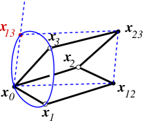
Figure 4. Construction of the point $x_{13}$ from points $x_{0}$, $x_{1}$, $x_{2}$, $x_{3}$, $x_{12}$ and $x_{23}$. It belongs to the intersection line of two planes $\langle x_{0},x_{1},x_{3}\rangle$ with the plane $\langle x_{0},x_{12},x_{23}\rangle$. Because the line intersects the quadric at $x_{0}$, it must have also the second intersection point.

Remark.

It is easy to see that, unlike in the case of isothermic lattices, three vertices of a quadrilateral of trapezoidal lattice in a quadric [8] determine the forth vertex.

Proposition 10.

A quadrilateral lattice in a quadric $x:{\mathbb{Z}}^{N}\to\mathcal{Q}\subset{\mathbb{P}}^{M}$ satisfying the local irreducibility condition is a generalized isothermic lattice if and only if there exist functions $\alpha^{i}:{\mathbb{Z}}\to{\mathbb{R}}$ of single arguments $n_{i}$ such that the cross-ratios $\lambda^{ij}=\mathrm{cr}(x_{(i)},x_{(j)};x,x_{(ij)})$ can be factorized as follows

(3.11) $$\lambda^{ij}=\frac{\alpha^{i}}{\alpha^{j}},\qquad 1\leq i<j\leq N.$$

Proof.

Equations (3.1) and (3.8) can be rewritten as

(3.12) $$\lambda^{ij}\lambda^{jk}=\lambda^{ik},\quad 1\leq i<j<k\leq N,$$

and

(3.13) $$\lambda^{ij}=\lambda^{ij}_{(k)},\quad\lambda^{jk}=\lambda^{jk}_{(i)},\quad\lambda^{ik}=\lambda^{ik}_{(j)},\quad 1\leq i<j<k\leq N;$$

notice their consistency with the general system (2.4).

Equations (3.12)-(3.13) imply that cross-ratios of two dimensional sub-lattices of the generalized isothermic lattice satisfy condition of the form (1.1), i.e.,

(3.14) $$\lambda^{ij}_{(ij)}\lambda^{ij}=\lambda^{ij}_{(i)}\lambda^{ij}_{(j)},\quad 1\leq i<j\leq N.$$

For a fixed pair $i,j$, the above relation can be resolved as in (3.11) (the first equation in (3.13) asserts that the functions $\alpha^{i}$ and $\alpha^{j}$ are the same for all $i,j$ sublattices). Finally, equations (3.12) imply the the functions $\alpha$ can be defined consistently on the whole lattice. ∎

For convenience of the Reader we present also the algebraic proof of the above properties of the generalized isothermic lattice (see also [8] for analogous results concerning T-nets in a quadric).

The algebraic proof.

Assume that solutions of the system of the discrete Moutard equations (2.1) satisfy the quadratic constraint

(3.15) $$({\boldsymbol{x}}|{\boldsymbol{x}})=0,$$

where $(\cdot|\cdot)$ is a symmetric nondegenerate bilinear form. Then the coefficients of the Moutard equations should be of the form

(3.16) $$f^{ij}=\frac{({\boldsymbol{x}}|{\boldsymbol{x}}_{(i)}-{\boldsymbol{x}}_{(j)})}{({\boldsymbol{x}}_{(i)}|{\boldsymbol{x}}_{(j)})},\quad 1\leq i<j\leq N.$$

Moreover by direct calculations one shows that

(3.17) $$({\boldsymbol{x}}_{(i)}|{\boldsymbol{x}})_{(j)}=({\boldsymbol{x}}_{(i)}|{\boldsymbol{x}}),\quad 1\leq i<j\leq N,$$

which implies that the products $({\boldsymbol{x}}_{(i)}|{\boldsymbol{x}})$, which we denote by $\alpha_{i}$, are functions of single variables $n_{i}$.

Consider the points $x,x_{(i)},x_{(j)}$ as the (projective) basis of the plane $\langle x,x_{(i)},x_{(j)}\rangle$. Then the homogeneous coordinates of points of the plane can be written as

(3.18) $${\boldsymbol{y}}=t{\boldsymbol{x}}+t_{i}{\boldsymbol{x}}_{(i)}+t_{j}{\boldsymbol{x}}_{(j)},\qquad(t,t_{i},t_{j})\in{\mathbb{R}}^{3}_{*},$$

modulo the standard common proportionality factor. In particular, the line $\langle x,x_{(i)}\rangle$ is given by equation $t_{j}=0$, and the line $\langle x,x_{(j)}\rangle$ is given by equation $t_{i}=0$. Due to the discrete Moutard equation (2.1) the line $\langle x,x_{(ij)}\rangle$ is given by equation $t_{i}+t_{j}=0$.

To find the cross-ratio $\mathrm{cr}(x_{(i)},x_{(j)};x,x_{(ij)})=\lambda^{ij}$ via lines of the planar pencil with the base point $x$ we need equation of the tangent to the conic $({\boldsymbol{y}}|{\boldsymbol{y}})=0$ at that point. It is easy to check that the conic is given by

(3.19) $$tt_{i}\alpha_{i}+tt_{j}\alpha_{j}+t_{i}t_{j}({\boldsymbol{x}}_{(i)}|{\boldsymbol{x}}_{(j)})=0.$$

The tangent to the conic at $x$ is then given by

(3.20) $$t_{i}\alpha_{i}+t_{j}\alpha_{j}=0,$$

which implies equation (3.11). ∎

Remark.

It should be mentioned the a similar quadratic reduction of the discrete Moutard equation (for $N=2$) appeared in a paper of Wolfgang Schief [52] under the name of discrete vectorial Calapso equation, as an integrable discrete vectorial analogue of the Calapso equation [10], which is of the fourth order and describes isothermic surfaces. It turns out that the discrete Calapso equation describes also the so called Bianchi reduction of discrete asymptotic surfaces [31].

3.2. Isothermic lattices in the Möbius sphere and the so called Clifford configuration

In [40] Konopelchenko and Schief observed that the ”complex cross-ratio definition” of the discrete isothermic surfaces, when extended to three dimensional lattices, is related with the so called Clifford configuration of circles (see Figure 5).

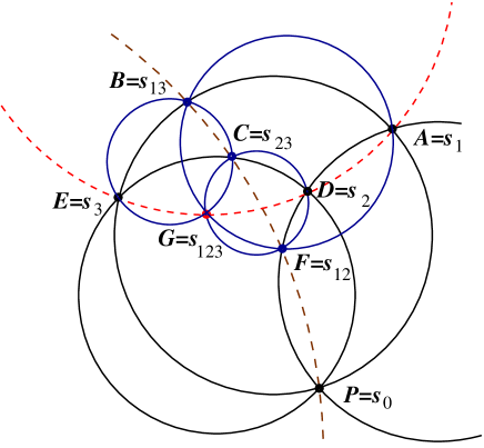
Figure 5. The so called Clifford configuration of circles (the second Miquel configuration)

In this Section we would like to explain that fact geometrically.

Our point of view on the Clifford configuration is closely related to the geometric definition of the isothermic lattice in the Möbius sphere. Therefore we start with another, less restrictive, configuration of circles on the plane, the Miquel configuration (see Figure 6), which provides geometric explanation of integrability of the circular lattice [13]. When the quadric in Lemma 3 is the standard sphere then the intersection curves of the planes of the quadrilaterals with the sphere are circles. After the stereographic projection from a generic point of the sphere we obtain the classical Miquel theorem [43], which can be stated as follows (given three distinct points $a$, $b$ and $c$, by $C(a,b,c)$ we denote the unique circle-line passing through them).

Theorem 11 (The Miquel configuration).

Given four coplanar points $s_{0}$, $s_{i}$, $i=1,2,3$. On each circle $C(s_{0},s_{i},s_{j})$, $1\leq i<j\leq 3$ choose a point, denoted correspondingly by $s_{ij}$. Then there exists the unique point $s_{123}$ which belongs simultaneously to the three circles $C(s_{1},s_{12},s_{13})$, $C(s_{2},s_{12},s_{23})$ and $C(s_{3},s_{13},s_{23})$.

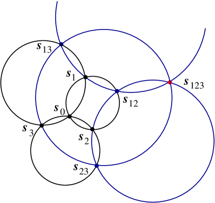
Figure 6. The (first) Miquel configuration of circles

The additional assumption about coplanarity of the points $x_{0}$, $x_{12}$, $x_{13}$, $x_{23}$ on the sphere is then equivalent to the additional assumption about concircularity of the corresponding points $s_{0}$, $s_{12}$, $s_{13}$, $s_{23}$. In view of Lemma 2 we obtain therefore another configuration of circles, the so called Clifford configuration, which can be described as follows.

Theorem 12 (The so called Clifford configuration).

Under hypotheses of Theorem 11 assume that the points $s_{0}$, $s_{12}$, $s_{13}$, $s_{23}$ are concircular, then the points $s_{1}$, $s_{2}$, $s_{3}$ and $s_{123}$ are concircular as well.

Remark.

The original Clifford’s formulation of the above result was more symmetric. Its relation to Theorem 12 is analogous to relation of the Cox theorem to Lemma 2. We remark that although the above theorem is usually attributed (see for example [15]) to Wiliam Clifford [14] it appeared in much earlier paper [43] of Auguste Miquel, where we read as Thèorème II the following statement: Lorsqu’un quadrilatère complet curviligne ABCDEF est formé par quatre arcs de cercle AB, BC, CD, DA, qui se coupent tous quatre en un même point P, si l’on circonscrit des circonférences de cercle à chacun des quatre triangles curvilignes que forment les côtés de ce quadrilatère, les circonférences de cercle AFB, EBC, DCF, DAE ainsi obtenues se couperont toutes quatre en un même point G. Points on Figure 5 are labelled in double way to visualize simultaneously the configuration in formulation of Theorem 12 and in Miquel’s formulation.

4. The Darboux transformation of the generalized isotermic lattice

4.1. The fundamental, Moutard and Ribaucour transformations

Usually, on the discrete level there is no essential difference between integrable lattices and their transformations. The analogue of the fundamental transformation of Jonas for quadrilateral lattices is defined as construction of a new level of the lattice [30] keeping the basic property of planarity of elementary quadrilaterals. Below we recall the relevant definitions of the fundamental transformation and its important reductions – the BQL reduction [23] (algebraically equivalent to the Moutard transformation [46]), and the QQL reduction [20] called the Ribaucour transformation.

Definition 5.

The fundamental transform of a quadrilateral lattice $x:{\mathbb{Z}}^{N}\to{\mathbb{P}}^{M}$ is a new quadrilateral lattice $\hat{x}:{\mathbb{Z}}^{N}\to{\mathbb{P}}^{M}$ constructed under assumption that for any point $x$ of the lattice and any direction $i$, the four points $x$, $x_{(i)}$, $\hat{x}$ and $\hat{x}_{(i)}$ are coplanar.

Definition 6.

The fundamental transformation of a B-quadrilateral lattice $x:{\mathbb{Z}}^{N}\to{\mathbb{P}}^{M}$ constructed under additional assumption that for any point $x$ of the lattice and any pair $i,j$ of different directions, the four points $x$, $x_{(ij)}$, $\hat{x}_{(i)}$ and $\hat{x}_{(j)}$ are coplanar is called the BQL (Moutard) reduction of the fundamental transformation of $x$.

Algebraic description of the above transformation is given as follows [46]. Given solution ${\boldsymbol{x}}$ of the system of discrete Moutard equations (2.1) and given its scalar solution $\theta$, then the solution $\hat{{\boldsymbol{x}}}$ of the system

(4.1) $$\hat{\boldsymbol{x}}_{(i)}-{\boldsymbol{x}}=\frac{\theta}{\theta_{(i)}}\left(\hat{\boldsymbol{x}}-{\boldsymbol{x}}_{(i)}\right),$$

satisfies equations (2.1) with the new potential

(4.2) $$\hat{f}^{ij}=f^{ij}\frac{\theta_{(i)}\theta_{(j)}}{\theta\theta_{(ij)}},\qquad i<j,$$

and new $\tau$-function

(4.3) $$\hat{\tau}=\theta\tau.$$

Definition 7.

The fundamental transformation of a quadrilateral lattice $x:{\mathbb{Z}}^{N}\to\mathcal{Q}\subset{\mathbb{P}}^{M}$ in a quadric, constructed under additional assumption that also $\hat{x}$ satifies the same quadratic constraint is called the Riboucour transformation of $x$.

4.2. The Darboux transformation

Definition 8.

The fundamental transformation of a generalized isothermic lattice which is simultaneously the Ribaucour and the Moutard transformation is called the Darboux transformation.

Notice that there is essentially no difference between the Darboux transformation and construction of a new level of the generalized isothermic lattice. Therefore, given points $x$, $x_{(i)}$, $x_{(j)}$, $x_{(ij)}$, $i\neq j$, of the initial lattice, and given points $\hat{x}$, $\hat{x}_{(j)}$ of its Darboux transform then the point $\hat{x}_{(i)}$ is determined by the ”half-hexahedron construction” visualized on Figure 4, i.e., $\hat{x}_{(i)}$ is the intersection point of the line $\langle x,x_{(i)},\hat{x}\rangle\cap\langle x,x_{(ij)},\hat{x}_{(j)}\rangle$ with the quadric. Moreover, Lemma 5 implies

(4.4) $$\mathrm{cr}(x_{(i)},\hat{x};x,\hat{x}_{(i)})=\mathrm{cr}(x_{(i)},x_{(j)};x,x_{(ij)})\mathrm{cr}(x_{(j)},\hat{x};x,\hat{x}_{(j)}),$$

while Corollary 8 gives

(4.5) $$\mathrm{cr}(\hat{x}_{(i)},\hat{x}_{(j)};\hat{x},\hat{x}_{(ij)})=\mathrm{cr}(x_{(i)},x_{(j)};x,x_{(ij)}).$$

The algebraic derivation of the above results is given below. The Darboux transformations of the discrete isothermic surfaces in the light-cone description were discussed in a similar spirit in [8].

Proposition 13.

If $\hat{x}:{\mathbb{Z}}^{N}\to\mathcal{Q}\subset{\mathbb{P}}^{M}$ is a Darboux transform of the generalized isothermic lattice $x:{\mathbb{Z}}^{N}\to\mathcal{Q}\subset{\mathbb{P}}^{M}$ then the product $(\hat{{\boldsymbol{x}}}|{\boldsymbol{x}})$ of their homogeneous coordinates in the gauge of the linear problem (2.1) and the corresponding Moutard transformation (4.1), with respect to the bilinear form $(\cdot|\cdot)$ defining the quadric $\mathcal{Q}$, is constant.

Proof.

The homogeneous coordinates ${\boldsymbol{x}}$ and $\hat{{\boldsymbol{x}}}$ in the Moutard transformation satisfy equation of the form

(4.6) $$\hat{{\boldsymbol{x}}}_{(i)}-{\boldsymbol{x}}=f^{i}(\hat{{\boldsymbol{x}}}-{\boldsymbol{x}}_{(i)}),\qquad 1\leq i\leq N,$$

with appropriate functions $f^{i}:{\mathbb{Z}}^{N}\to{\mathbb{R}}$. The quadratic condition $(\hat{{\boldsymbol{x}}}_{(i)}|\hat{{\boldsymbol{x}}}_{(i)})=0$ together with other quadratic conditions give

(4.7) $$f^{i}=\frac{({\boldsymbol{x}}|\hat{{\boldsymbol{x}}}-{\boldsymbol{x}}_{(i)})}{(\hat{{\boldsymbol{x}}}|{\boldsymbol{x}}_{(i)})},$$

which implies $(\hat{{\boldsymbol{x}}}_{(i)}|{{\boldsymbol{x}}}_{(i)})=(\hat{{\boldsymbol{x}}}|{\boldsymbol{x}})$. ∎

Notice the above proof goes along the corresponding reasoning in the first part of the algebraic proof of Proposition 10. The analogous reasoning as in its second part gives the following statement.

Corollary 14.

Under hypothesis of Proposition 13 denote $\zeta=(\hat{{\boldsymbol{x}}}|{\boldsymbol{x}})$ and $\lambda^{i}=\mathrm{cr}(\hat{x},x_{(i)};x,\hat{x}_{(i)})$ then equations (3.11) and (3.12) should be replaced by

(4.8) $$\lambda^{i}=\frac{\zeta}{\alpha_{i}},\qquad\lambda^{i}\lambda^{ij}=\lambda^{j}.$$

The above reasoning can be reversed giving the algebraic way to find the Darboux transform of a given generalized isothermic lattice.

Theorem 15.

Given a solution ${\boldsymbol{x}}:{\mathbb{Z}}^{N}\to{\mathbb{R}}^{M+1}_{*}$ of the system of Moutard equations (2.1) satisfying the constraint $({\boldsymbol{x}}|{\boldsymbol{x}})=0$, considered as homogeneous coordinates of generalized isothermic lattice $x:{\mathbb{Z}}^{N}\to\mathcal{Q}\subset{\mathbb{P}}^{M}$, denote $\alpha_{i}=({\boldsymbol{x}}_{(i)}|{\boldsymbol{x}})$. Given a point $[\hat{{\boldsymbol{x}}}_{0}]=\hat{x}_{0}\in\mathcal{Q}$, denote $\zeta=(\hat{{\boldsymbol{x}}}_{0}|{\boldsymbol{x}}(0))$. Then there exists unique solution of the linear system

(4.9) $$\hat{{\boldsymbol{x}}}_{(i)}={\boldsymbol{x}}+\frac{\zeta-\alpha_{i}}{(\hat{{\boldsymbol{x}}}|{\boldsymbol{x}}_{(i)})}(\hat{{\boldsymbol{x}}}-{\boldsymbol{x}}_{(i)}),\qquad,\quad 1\leq i\leq N,$$

with initial condition $\hat{{\boldsymbol{x}}}(0)=\hat{{\boldsymbol{x}}}_{0}$ which gives the Darboux transform of the lattice $x$. In particular

(4.10) $$\mathrm{cr}(\hat{x},x_{(i)};x,\hat{x}_{(i)}) =\frac{\zeta}{\alpha_{i}}$$

(4.11) $$\mathrm{cr}(\hat{x}_{(i)},\hat{x}_{(j)};\hat{x},\hat{x}_{(ij)}) =\mathrm{cr}(x_{(i)},x_{(j)};x,x_{(ij)})=\frac{\alpha^{i}}{\alpha^{j}}.$$

Before proving the Theorem let us state a Lemma relating the parameter $\zeta$ of the Darboux transformation with the functional parameter $\theta$ of the Moutard transformation (4.1).

Lemma 16.

Under hypotheses of Theorem 15 the solution $\theta$ of the system

(4.12) $$\theta_{(i)}=\theta\frac{(\hat{{\boldsymbol{x}}}|{\boldsymbol{x}}_{(i)})}{\zeta-\alpha_{i}},\qquad\quad 1\leq i\leq N,$$

satisfies the system of discrete Moutard equations (2.1) with the coefficients given by (3.16).

Proof of the Lemma.

By direct verification. Notice that both ways to calculate $\theta_{(ij)}$, $i\neq j$, from $\theta$ give the same result, and to do that we do not use compatibility of the system (4.9). ∎

Proof of the Theorem.

By direct calculation one can check that the system (4.9) preserves the constraints $(\hat{{\boldsymbol{x}}}|\hat{{\boldsymbol{x}}})=0$ and $(\hat{{\boldsymbol{x}}}|{\boldsymbol{x}})=\zeta$, moreover $(\hat{{\boldsymbol{x}}}_{(i)}|\hat{{\boldsymbol{x}}})=({\boldsymbol{x}}_{(i)}|{\boldsymbol{x}})$. Compatibility of the system (4.9) can be checked by direct calculation, but in fact it is the consequence of Lemma 16 and properties of the Moutard transformation (4.1). ∎

Remark.

Notice that because there is essentially no diffrence between the lattice directions and the transformation directions, the tranformation equations (4.9) can be guessed by keeping the Moutard-like form supplementing it by calculation of the coefficient $f^{i}$ from the quadratic constraint. We will use this observation in the next Section where we consider the permutability principle for the Darboux transformations of generalized isothermic lattices.

4.3. The Bianchi permutability principle

The original Bianchi superposition principle for the Darboux transformations of the isothermic surfaces reads as follows [2]: Se dalla superficie isoterma $S$ si ottengono due nuove superficie isoterme $S_{1}$, $S_{2}$ mediante le trasformazioni di Darboux $D_{m_{1}}$, $D_{m_{2}}$ a costanti $m_{1}$, $m_{2}$ differenti, esiste una quarta superficie isoterma $\overline{S}$, pienamente determinata e costruibile in termini finiti, che è legata alla sua volta alle medesime superficie $S_{1}$, $S_{2}$ da due trasformazioni di Darboux $\overline{D}_{m_{2}}$, $\overline{D}_{m_{1}}$ colle costanti invertite $m_{2}$, $m_{1}$.

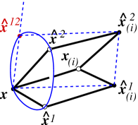
Figure 7. Geometric construction of the superposition of two Darboux transformations

Its version for generalized isothermic lattices can be formulated analogously.

Proposition 17.

When from given generalized isothermic lattice $x$ there were constructed two new isothermic lattices $\hat{x}^{1}$ and $\hat{x}^{2}$ via the Darboux transformations with different parameters $\zeta_{1}$ and $\zeta_{2}$, then there exists the unique forth generalized isothermic lattice $\hat{x}^{12}$, determined in algebraic terms from the three previous ones, which is connected with two intermediate lattices $\hat{x}^{1}$ and $\hat{x}^{2}$ via two Darboux transformations with reversed parameters $\zeta_{2}$, $\zeta_{1}$.

Proof.

The algebraic properties of the B-reduction of the fundamental transformation (the discrete Moutard transformation) imply that in the gauge of the linear problem (2.1) and of the transformation equations (4.1) the superposition of two such transformations reads

(4.13) $$\hat{{\boldsymbol{x}}}^{12}-{\boldsymbol{x}}=f(\hat{{\boldsymbol{x}}}^{1}-\hat{{\boldsymbol{x}}}^{2}),$$

where $f$ is an appropriate function [46, 23]. Because of the additional quadratic constraints the function is given by (compare also equations (3.16) and (3.16))

(4.14) $$f=\frac{({\boldsymbol{x}}|\hat{{\boldsymbol{x}}}^{1}-\hat{{\boldsymbol{x}}}^{2})}{(\hat{{\boldsymbol{x}}}^{1}|\hat{{\boldsymbol{x}}}^{2})}.$$

The lattice $\hat{x}^{12}$ with homogeneous coordinates given by (4.13) and (4.14) is superposition of two Darboux transforms. Finally, direct calculation shows that

(4.15) $$(\hat{{\boldsymbol{x}}}^{12}|\hat{{\boldsymbol{x}}}^{2})=(\hat{{\boldsymbol{x}}}^{1}|{\boldsymbol{x}})=\zeta_{1},\qquad(\hat{{\boldsymbol{x}}}^{12}|\hat{{\boldsymbol{x}}}^{1})=(\hat{{\boldsymbol{x}}}^{2}|{\boldsymbol{x}})=\zeta_{2}.$$

∎

Corollary 18.

The final algebraic superposition formula reads

(4.16) $$\hat{{\boldsymbol{x}}}^{12}-{\boldsymbol{x}}=\frac{\zeta_{1}-\zeta_{2}}{(\hat{{\boldsymbol{x}}}^{1}|\hat{{\boldsymbol{x}}}^{2})}(\hat{{\boldsymbol{x}}}^{1}-\hat{{\boldsymbol{x}}}^{2}),$$

while the cross-ratio of the four corresponding points calculated with respect to the conic intersection of the plane $\langle x,\hat{x}^{1},\hat{x}^{2}\rangle$ and the quadric is given by

(4.17) $$\mathrm{cr}(\hat{x}^{1},\hat{x}^{2};x,\hat{x}^{12})=\frac{\zeta_{1}}{\zeta_{2}}.$$

To find the lattice $\hat{x}^{12}$ geometrically we can use again the ”half-hexahedron construction” in the new context visualized on Figure 7 (compare with Figure 4). Moreover, Lemma 5 gives

(4.18) $$\mathrm{cr}(\hat{x}^{1},\hat{x}^{2};x,\hat{x}^{12})=\mathrm{cr}(\hat{x}^{1},x_{(i)};x,\hat{x}^{1}_{(i)})\,\mathrm{cr}(x_{(i)},\hat{x}^{2};x,\hat{x}^{2}_{(i)}),$$

which, due to equation (4.10), is in agreement with (4.17).

5. Two dimensional generalized isothermic lattice

In the previous Sections we were mainly interested in generalized isothermic lattices of dimension greater then two. However, simultaneous application of the B-constraint and the quadratic constraint lowers dimensionality of the lattice (in the sense of the initial boundary value problem). One can see it from Figure 4, which implies that two intersecting strips made of planar quadrialterals with vertices in a quadric (see Figure 8) can be extended to a two dimensional quadrilateral lattice in the quadric. Because of Lemma 5 such lattice satisfies Steiner’s version of the cross-ratio constraint (1.1).

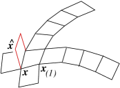
Figure 8. Two intersecting initial strips of a two dimensional generalized isothermic lattice allow to build all the lattice. The additional transverse quadrilateral allows to build the lattice (together wih its Darboux transform) in a three dimensional fashion

One can define however geometrically two dimensional generalized isothermic lattices (generalized discrete isothermic surfaces) without using the three dimensional construction. An important tool here is the projective interpretation of the discrete Moutard equation [33] as representing quadrilateral lattice with additional linear relation between any of its points $x$ and its four second-order neighbours $x_{(\pm 1\pm 2)}$. Geometrically, such five points of a two dimensional B-quadrilateral lattice are contained in a subspace of dimension three; for generic two dimensional quadrilateral lattice such points are contained in a subspace of dimension four. To exclude further degenerations we assume that no of the four points $x_{\pm 1}$, $x_{\pm 2}$ belongs to that three dimensional subspace.

Definition 9.

A two dimensional B-quadrilateral lattice in a hyperquadric $x:{\mathbb{Z}}^{2}\to\mathcal{Q}\subset{\mathbb{P}}^{M}$ satisfying the local irreducibility condition is called a generalized discrete isothermic surface.

Remark.

Notice that the above Definition gives (the conclusion was drawn by Alexander Bobenko) a geometric characterization of the classical discrete isothermic surfaces of Bobenko and Pinkall. Mainly, the non-trivial intersection of a three dimensional subspace with the Möbius sphere is a two dimensional sphere. After the stereographic projection, which preserves co-sphericity of points, a discrete isothermic surface in the Möbius (hyper)sphere gives circular two dimensional lattice $s:{\mathbb{Z}}^{2}\to{\mathbb{E}}^{M}$ such that for any of its points $s$ there exists a sphere containig the point and its four second-order neighbours $s_{(\pm 1\pm 2)}$.

Notice that, actually, all calculations where we used simultaneously both the discrete Moutard equation and the quadratic constraint (algebraic proofs of Proposition 10, Theorem 15 and Proposition 17) remain true for $N=2$. Therefore the corresponding results on the cross-ratio characterization of generalized discrete isothermic surfaces, their Darboux transformation and the Bianchi superposition principle are still valid.

To complete this Section let us present the geometric construction of a generalized discrete isothermic surface (see Figure 9).

Figure 9. Geometric construction of generalized discrete isothermic surfaces

The basic step of the construction, which allows to build the generalized discrete isothermic surface from two initial quadrilateral strips in a quadric in a two dimensional fashion can be discribed as follows. Consider the four dimensional subspace $V_{4}=\langle x,x_{(1)},x_{(2)},x_{(-1)},x_{(-2)}\rangle$, where the basic step takes place. Denote by $V_{3}=\langle x,x_{(-1-2)},x_{(-12)},x_{(1-2)}\rangle$ its three dimensional subspace passing through the points $x$, $x_{(-1-2)}$, $x_{(-12)}$ and $x_{(1-2)}$, and by $V_{2}=\langle x,x_{(1)},x_{(2)}\rangle$ the plane of the elementary quatrilateral whose fourth vertex $x_{12}$ we are going to find. In the construction of the two dimensional B-quadrilateral lattice the vertex must belong to the line $V_{1}=V_{3}\cap V_{2}$. In our case it should also belong to the conic $\mathcal{C}=V_{2}\cap\mathcal{Q}$. Because the conic contains already one point $x$ of the line $V_{1}$, the second point is unique. Notice that although the points $x_{(-1)}$ and $x_{(-2)}$ do not play any role in the construction, they can be easily recovered in a similar way as above.

6. Conclusions and discussion

In the paper we defined new integrable reduction of the lattice of planar quadrilaterals, which contains as a particular example the discrete isothermic surfaces. We studied, by using geometric and algebraic means, various aspects of such generalized isothermic lattices. In particular, we defined the (analogs of the) Darboux transformations for the lattices and we showed the corresponding permutablity principle.

The theory of integrable systems is deeply connected with results of geometers of the turn of XIX and XX centuries. The relation of integrability and geometry is even more visible on the discrete level, where into the game there enter basic results of the projective geometry. In our presentation of the generalized isothermic lattices the basic geometric results were a variant of the Möbius theorem and the generalization of the Miquel theorem to arbitrary quadric, which combined together gave the corresponding generalization of the Clifford theorem (known already to Miquel). An important tool in our research was also Steiner’s description of conics and the geometric properties of von Staudt’s algebra (see Appendix A).

Appendix A The cross-ratio and the projective structure of a conic

For convenience of the Reader we have collected some facts from projective geometry (see, for example [49, 54]) used in the main text of the paper. Let $a,b,c$ be distinct points of the projective line $D$ over the field ${\mathbb{K}}$. Given $d\in D$, the cross-ratio $\mathrm{cr}(a,b;c,d)$ of the four points $a,b,c,d$ is defined as $h(d)\in\hat{\mathbb{K}}={\mathbb{K}}\cup\{\infty\}$ where $h$ is the unique projective transformation $D\to\hat{\mathbb{K}}$ that takes $a$, $b$ and $c$ to $\infty$, $0$ and $1$, respectively. For $D=\hat{\mathbb{K}}$, with the usual conventions about operations with $0$ and $\infty$, the cross-ratio is given by

(A.1) $$\mathrm{cr}(a,b;c,d)=\frac{(c-a)(d-b)}{(c-b)(d-a)}.$$

Denote by $\boldsymbol{a}$ and $\boldsymbol{b}$ homogenous coordinates of the points $a$ and $b$. If the homogenous coordinates of the points $c$ and $d$ collinear with $a$, $b$ are, respectively, $\boldsymbol{c}=\alpha\boldsymbol{a}+\beta\boldsymbol{b}$ and $\boldsymbol{d}=\gamma\boldsymbol{a}+\delta\boldsymbol{b}$, then

(A.2) $$\mathrm{cr}(a,b;c,d)=\frac{\beta\gamma}{\alpha\delta}.$$

Let $D$ and $D^{\prime}$ be projective lines, $a,b,c,d$ distinct points on $D$, and $a^{\prime},b^{\prime},c^{\prime},d^{\prime}$ distinct points on $D^{\prime}$. There exists a projective transformation $u:D\to D^{\prime}$ taking $a,b,c,d$ into $a^{\prime},b^{\prime},c^{\prime},d^{\prime}$, respectively, if and only if the cross-ratios $\mathrm{cr}(a,b;c,d)$ and $\mathrm{cr}(a^{\prime},b^{\prime};c^{\prime},d^{\prime})$ are equal.

Figure 10. Multiplication of cross-ratios on the line

Following von Staudt one can perform geometrically algebraic operations on cross-ratios (see [54] for details). We will be concerned with geometric multiplication, which can be considered as ”projectivization” of the Thales theorem – see the self-explanatory Figure 10.

The planar pencil of lines has the natural projective structure inherited from any line not intersecting its base. Let $\mathcal{C}$ be an irreducible conic in a projective plane, and $a\in\mathcal{C}$ a point. To each line $D$ of the pencil $F_{a}$ of the base $a$, we associate the second point where $D$ intersects $\mathcal{C}$ (see Figure 11); we denote this point by $j_{a}(D)$. When $D$ is the tangent to $\mathcal{C}$ at $a$, let $j_{a}(D)$ be the point $a$. Thus $j_{a}$ is a bijection from $F_{a}$ to $\mathcal{C}$. If $b$ is another point on $\mathcal{C}$, the composition $j_{b}^{-1}\circ j_{a}$ is a projective transformation from $F_{a}$ to $F_{b}$.

Figure 11. The projective structure of a conic

Thus the bijection from $F_{a}$ to $\mathcal{C}$ allows us to transport to $\mathcal{C}$ the projective structure of $F_{a}$. This structure does not depend on the point $a$. Conversely, any projective transformation between two pencils defines a conic.

Finally we present the relation between the complex cross-ratio of the Möbius geometry, and Steiner’s conic cross-ratio.

Proposition 19.

Four points $a,b,c,d\in\hat{\mathbb{C}}$ are cocircular or collinear if and only if their cross-ratio $\mathrm{cr}(a,b;c,d)_{\mathbb{C}}$ computed in $\hat{\mathbb{C}}$, is real. The cross-ratio $\mathrm{cr}(a,b;c,d)_{\mathbb{C}}$ is equal to the cross-ratio $\mathrm{cr}(a,b;c,d)$ computed using the real projective line structure of the line or the circle considered as a conic.

Appendix B Auxiliary calculations

In this Appendix we would like to prove the ”cross-ratio” characterization (Proposition 4) of locally irreducible quadrilateral lattices in quadrics, and then to give algebraic proof of the basic Lemma 5. It turns out that in the course of our calculations will give also algebraic ”down to earth” proofs of the basic Lemmas 1, 2 and 3.

Proposition 4 is immediate consequence of the following result.

Lemma 20.

Under hypotheses of Lemma 3 and irreducibility of the conics, being intersections of the planes of the quadrilaterals with the quadric, the cross-ratios (defined with respect to the conics) of points on opposite sides of the hexahedron are connected by the following equation

(B.1) $$\begin{split}\mathrm{cr}(x_{1},x_{2};x_{0},x_{12})&\,\mathrm{cr}(x_{13},x_{23};x_{3},x_{123})\mathrm{cr}(x_{2},x_{3};x_{0},x_{23})\,\mathrm{cr}(x_{12},x_{13};x_{1},x_{123})=\\ &=\mathrm{cr}(x_{1},x_{2};x_{0},x_{13})\,\mathrm{cr}(x_{13},x_{23};x_{2},x_{123}).\end{split}$$

Proof.

Let us choose the points $x_{0}$, $x_{1}$, $x_{2}$ and $x_{3}$ as the basis of projective coordinate system in the corresponding three dimensional subspace, i.e.,

$${\boldsymbol{x}}_{0}=[1:0:0:0],\quad{\boldsymbol{x}}_{1}=[0:1:0:0],\quad{\boldsymbol{x}}_{2}=[0:0:1:0],\quad{\boldsymbol{x}}_{3}=[0:0:0:1],$$

and denote by $[t_{0}:t_{1}:t_{2}:t_{3}]$ the corresponding homogeneous coordinates. For generic points $x_{ij}\in\langle x_{0},x_{i},x_{j}\rangle$, $1\leq i<j\leq 3$, with homogeneous coordinates

$${\boldsymbol{x}}_{12}=[a_{0}:a_{1}:a_{2}:0],\quad{\boldsymbol{x}}_{13}=[b_{0}:b_{1}:0:b_{3}],\quad{\boldsymbol{x}}_{23}=[c_{0}:0:c_{2}:c_{3}],$$

one obtains, via the standard linear algebra, equations of the planes $\langle x_{1},x_{12},x_{13}\rangle$, $\langle x_{2},x_{12},x_{23}\rangle$, $\langle x_{3},x_{13},x_{23}\rangle$ respectively,

(B.2) $$a_{2}b_{3}t_{0}= a_{0}b_{3}t_{2}+b_{0}a_{2}t_{3},$$

(B.3) $$a_{1}c_{3}t_{0}= a_{0}c_{3}t_{1}+c_{0}a_{1}t_{3},$$

(B.4) $$b_{1}c_{2}t_{0}= b_{0}c_{2}t_{1}+c_{0}b_{1}t_{2}.$$

The intersection point $x_{123}$ of the planes has the following coordinates ${\boldsymbol{x}}_{123}=[y_{0}:y_{1}:y_{2}:y_{3}]$

(B.5) $$\begin{split}y_{0}=&a_{0}b_{0}c_{0}\left(\frac{1}{a_{2}b_{1}c_{3}}+\frac{1}{a_{1}b_{3}c_{2}}\right),\\ y_{1}=&\frac{b_{0}c_{0}}{b_{3}c_{2}}+\frac{a_{0}c_{0}}{a_{2}c_{3}}-\frac{c_{0}^{2}}{c_{2}c_{3}},\\ y_{2}=&\frac{a_{0}b_{0}}{a_{1}b_{3}}+\frac{b_{0}c_{0}}{b_{1}c_{3}}-\frac{b_{0}^{2}}{b_{1}b_{3}},\\ y_{3}=&\frac{a_{0}c_{0}}{a_{1}c_{2}}+\frac{a_{0}b_{0}}{a_{2}b_{1}}-\frac{a_{0}^{2}}{a_{1}a_{2}}.\end{split}$$

Up to now we have not used the additional quadratic restriction, and what we have done was just the algebraic proof of Lemma 1.

Any quadric ${\mathcal{Q}}$ passing through $x_{0}$, $x_{1}$, $x_{2}$ and $x_{3}$ must have equation of the form

(B.6) $$a_{01}t_{0}t_{1}+a_{02}t_{0}t_{2}+a_{03}t_{0}t_{3}+a_{12}t_{1}t_{2}+a_{13}t_{1}t_{3}+a_{23}t_{2}t_{3}=0.$$

The homogeneous coordinates of the points $x_{12}$, $x_{23}$ and $x_{13}$ can be parametrized in terms of the corresponding cross-ratios $\lambda=\mathrm{cr}(x_{1},x_{2};x_{0},x_{12})$, $\nu=\mathrm{cr}(x_{2},x_{3};x_{0},x_{23})$ and $\mu=\mathrm{cr}(x_{1},x_{3};x_{0},x_{13})$ as

(B.7) $${\boldsymbol{x}}_{12} =\Big{[}\,\frac{\lambda a_{12}}{1-\lambda}\,:\,-\lambda a_{02}\,:\,a_{01}\,:\,0\,\Big{]},$$

(B.8) $${\boldsymbol{x}}_{23} =\Big{[}\,\frac{\nu a_{23}}{1-\nu}\,:\,0\,:\,-\nu a_{03}\,:\,a_{02}\,\Big{]},$$

(B.9) $${\boldsymbol{x}}_{13} =\Big{[}\,\frac{\mu a_{13}}{1-\mu}\,:\,-\mu a_{03}\,:\,0\,:\,a_{01}\,\Big{]}.$$

We will only show how to find the homogeneous coordinates of $x_{12}$ in terms of $\lambda$. Let us parametrize points of the conic

(B.10) $$a_{01}t_{0}t_{1}+a_{02}t_{0}t_{2}+a_{12}t_{1}t_{2}=0,$$

being intersection of the quadric (B.6) with the plane $t_{3}=0$, by the planar pencil with base at $x_{0}$. The point $x_{0}$ corresponds to the tangent to the conic at $x_{0}$

$$a_{01}t_{1}+a_{02}t_{2}=0,$$

while the points $x_{1}$ and $x_{2}$ correspond to lines $t_{2}=0$ and $t_{1}=0$, respectively. The line $\langle x_{0},x_{12}\rangle$ must have equation (see equation (A.2) in Appendix A) of the form

$$a_{01}t_{1}+\lambda a_{02}t_{2}=0,$$

which inserted into equation (B.10) of the conic gives, after exluding the point $x_{0}$, the homogeneous coordinates of the point $x_{12}$.

Inserting expressions (B.7), (B.8) and (B.9) into formulas (B.5) we obtain homogeneous coordinates $[y_{0}:y_{1}:y_{2}:y_{3}]$ of the point $x_{123}$ parametrized in terms of the cross-ratios $\lambda$, $\nu$, $\mu$

(B.11) $$\begin{split}y_{0}=&\frac{a_{12}a_{23}a_{13}}{a_{01}a_{02}a_{03}}\frac{\lambda\nu-\mu}{(1-\lambda)(1-\mu)(1-\nu)},\\ y_{1}=&\frac{a_{23}}{1-\nu}\left(\frac{a_{13}}{a_{01}a_{03}}\frac{\mu}{1-\mu}-\frac{a_{23}}{a_{02}a_{03}}\frac{\nu}{1-\nu}-\frac{a_{12}}{a_{01}a_{02}}\frac{\lambda\nu}{1-\lambda}\right),\\ y_{2}=&\frac{a_{13}}{1-\mu}\left(-\frac{a_{13}}{a_{01}a_{03}}\frac{\mu}{1-\mu}+\frac{a_{23}}{a_{02}a_{03}}\frac{\nu}{1-\nu}+\frac{a_{12}}{a_{01}a_{02}}\frac{\mu}{1-\lambda}\right),\\ y_{3}=&\frac{a_{12}}{1-\lambda}\left(\frac{a_{13}}{a_{01}a_{03}}\frac{\lambda}{1-\mu}-\frac{a_{23}}{a_{02}a_{03}}\frac{1}{1-\nu}-\frac{a_{12}}{a_{01}a_{02}}\frac{\lambda}{1-\lambda}\right).\end{split}$$

One can check that such expressions do satisfy the quadric equation (B.6), i. e., we have obtained the direct proof of Lemma 3 under additional assumption of ireducibility of the conics.

Further calculations give the cross-ratios on remaining three sides of the hexahedron

$$\mathrm{cr}(x_{13},x_{23};x_{3},x_{123}) =-\frac{\mu(1-\nu)a_{13}y_{1}}{\nu(1-\mu)a_{23}y_{2}},$$

(B.12) $$\mathrm{cr}(x_{12},x_{13};x_{1},x_{123}) =-\frac{(1-\mu)a_{12}y_{2}}{(1-\lambda)a_{13}y_{3}},$$

$$\mathrm{cr}(x_{12},x_{23};x_{2},x_{123}) =\lambda\frac{(1-\nu)a_{12}y_{1}}{(1-\lambda)a_{23}y_{3}},$$

with $y_{i}$ given by (B.11), which implies equation (B.1). ∎

Algebraic proof of Lemma 5.

We can express coplanarity of four points in ${\mathbb{P}}^{3}$ as vanishing of the determinant of the matrix formed by their homogeneous coordinates. In notation of the proof above (up to equation (B.5)) we have

(B.13) $$y_{0}=\det\left({\boldsymbol{x}}_{123}\>{\boldsymbol{x}}_{1}\>{\boldsymbol{x}}_{2}\>{\boldsymbol{x}}_{3}\right)=\frac{a_{0}b_{0}c_{0}}{a_{1}a_{2}b_{1}b_{3}c_{2}c_{3}}\det\left({\boldsymbol{x}}_{0}\>{\boldsymbol{x}}_{12}\>{\boldsymbol{x}}_{23}\>{\boldsymbol{x}}_{13}\right),$$

which implies the statement of Lemma 2.

Finally, when vertices of the hexahedron are contained in the quadric, condition $y_{0}=0$ inserted into equation (B.11) gives $\mu=\lambda\nu$. ∎

References

- [1] J. Bertrand, Mémoire sur les surfaces isothermes orthogonales, J. Math. Pur. Appl. (Liouville J.) 9 (1844), 117-130, http://portail.mathdoc.fr/JMPA/.
- [2] L. Bianchi, Il teorema di permutabilità per le trasformazioni di Darboux delle superficie isoterme, Rend. Acc. Naz. Lincei 13 (1904), 359–367.
- [3] L. Bianchi, Lezioni di geometria differenziale, Zanichelli, Bologna, 1924.
- [4] A. Bobenko, Discrete conformal maps and surfaces, Symmetries and Integrability of Difference Equations (P. Clarkson and F. Nijhoff, eds.), Cambridge University Press, 1999, pp. 97–108.
- [5] A. Bobenko and U. Pinkall, Discrete surfaces with constant negative Gaussian curvature and the Hirota equation, J. Diff. Geom. 43 (1996), 527–611.
- [6] A. Bobenko and U. Pinkall, Discrete isothermic surfaces, J. Reine Angew. Math. 475 (1996), 187–208.
- [7] A. Bobenko and U. Pinkall, Discretization of surfaces and integrable systems, Discrete integrable geometry and physics, (A. Bobenko and R. Seiler, eds.), Clarendon Press, Oxford, 1999, pp. 3–58.
- [8] A. Bobenko and Yu. Suris, Discrete differential geometry. Consistency as integrability, arXiv:math.DG/0504358.
- [9] A. Bobenko and Yu. Suris, Isothermic surfaces in sphere geometries as Moutard nets, arXiv:math.DG/0610434.
- [10] P. Calapso, Sulla superficie a linee di curvature isoterme, Rend. Circ. Mat. Palermo 17 (1903), 275–286.
- [11] J. Cieśliński, The Bäcklund transformations for discrete isothermic surfaces, Symmetries and Integrability of Difference Equations (P. A. Clarkson and F. W. Nijhoff, eds.), University Press, Cambridge, 1999, pp. 109–121.
- [12] J. Cieśliński, P. Goldstein and A. Sym, Isothermic surfaces in as soliton surfaces, Phys. Lett. A 205 (1995), 37–43.
- [13] J. Cieśliński, A. Doliwa and P. M. Santini, The integrable discrete analogues of orthogonal coordinate systems are multidimensional circular lattices, Phys. Lett. A 235 (1997), 480–488.
- [14] W. K. Clifford, A synthetic proof of Miquels’s theorem, Oxford, Cambridge and Dublin Messenger of Math. 5 (1871), 124–141.
- [15] H. S. M. Coxeter, Introduction to geometry, Wiley, New York, 1969.
-
[16]
G. Darboux, Sur les surfaces isothermiques, Ann. Sc. É. N. S.,
16
(1899), 491–508,
http://www.numdam.org/item?id=ASENS_1899_3_16__491_0. - [17] G. Darboux, Leçons sur la théorie générale des surfaces. I–IV, Gauthier – Villars, Paris, 1887–1896.
- [18] G. Darboux, Leçons sur les systémes orthogonaux et les coordonnées curvilignes, Gauthier-Villars, Paris, 1910.
- [19] A. Doliwa, Geometric discretisation of the Toda system, Phys. Lett. A 234 (1997), 187–192.
- [20] A. Doliwa, Quadratic reductions of quadrilateral lattices, J. Geom. Phys. 30 (1999), 169–186.
- [21] A. Doliwa, Discrete asymptotic nets and W-congruences in Plücker line geometry, J. Geom. Phys. 39 (2001), 9–29.
- [22] A. Doliwa, Geometric discretization of the Koenigs nets, J. Math. Phys. 44 (2003), 2234–2249.
- [23] A. Doliwa, The B-quadrilateral lattice, its transformations and the algebro-geometric construction, J. Geom. Phys. 57 (2007), 1171–1192.
- [24] A. Doliwa, Generalized isothermic lattices, talk given at the Workshop ”Geometry and Integrable Systems” (Berlin, 3-7 June 2005), http://www.math.tu-berlin.de/geometrie/MISGAM/workshop2005/abstracts.html.
- [25] A. Doliwa and P. M. Santini, Integrable dynamics of a discrete curve and the Ablowitz-Ladik hierarchy, J. Math. Phys. 36 (1995), 1259–1273.
- [26] A. Doliwa and P. M. Santini, Multidimensional quadrilateral lattices are integrable, Phys. Lett. A 233 (1997), 365–372.
- [27] A. Doliwa and P. M. Santini, The symmetric, D-invariant and Egorov reductions of the quadrilateral lattice, J. Geom. Phys. 36 (2000), 60–102.
- [28] A. Doliwa and P. M. Santini, Integrable systems and discrete geometry, Encyclopedia of Mathematical Physics, (J. P. Françoise, G. Naber and T. S. Tsun, eds.) Vol. III, Elsevier, 2006, pp. 78-87.
- [29] A. Doliwa, S. V. Manakov and P. M. Santini, -reductions of the multidimensional quadrilateral lattice: the multidimensional circular lattice, Comm. Math. Phys. 196 (1998), 1–18.
- [30] A. Doliwa, P. M. Santini and M. Mañas, Transformations of quadrilateral lattices, J. Math. Phys. 41 (2000), 944–990.
- [31] A. Doliwa, M. Nieszporski and P. M. Santini, Asymptotic lattices and their integrable reductions I: the Bianchi and the Fubini-Ragazzi lattices, J. Phys. A 34 (2001), 10423–10439.
- [32] A. Doliwa, M. Nieszporski and P. M. Santini, Geometric discretization of the Bianchi system, J. Geom. Phys. 52 (2004), 217–240.
- [33] A. Doliwa, P. Grinevich, M. Nieszporski, and P. M. Santini, Integrable lattices and their sub-lattices: from the discrete Moutard (discrete Cauchy–Riemann) 4-point equation to the self-adjoint 5-point scheme, J. Math. Phys. (in press) arXiv:nlin.SI/0410046.
- [34] L. P. Eisenhart, Separable systems of Stäckel, Ann. of Math. 35 (1934), 284–305.
- [35] U. Hertrich-Jeromin, Introduction to Möbius differential geometry, Cambridge University Press, 2003.
- [36] U. Hertrich-Jeromin, T. Hoffmann and U. Pinkall, A discrete version of the Darboux transform for isothermic surfaces, Discrete integrable geometry and physics, (A. Bobenko and R. Seiler, eds.), Clarendon Press, Oxford, 1999, pp. 59–81.
-
[37]
T. Hoffmann, Discrete S-isothermic and S-cmc surfaces, talk given at
the Workshop ”Geometry and Integrable Systems”
(Berlin, 3-7 June 2005),
http://www.math.tu-berlin.de/geometrie/MISGAM/workshop2005/abstracts.html. - [38] P. Klimczewski, M. Nieszporski and A. Sym, Luigi Bianchi, Pasquale Calapso and solitons, Rend. Sem. Mat. Messina, Atti del Congresso Internazionale in onore di Pasquale Calapso, Messina 1998 (2000), 223–240.
- [39] B. G. Konopelchenko and W. K. Schief, Three-dimensional integrable lattices in Euclidean spaces: Conjugacy and orthogonality, Proc. Roy. Soc. London A 454 (1998), 3075–3104.
- [40] B. G. Konopelchenko and W. K. Schief, Conformal geometry of the (discrete) Schwarzian Davey-Stewartson II hierarchy, Glasgow Math. J. 47A (2005), 121–131.
- [41] G. Lamé, Mémoire sur les surfaces isothermes dans les corps solides homogènes en équilibre de température. J. Math. Pur. Appl. (Liouville J.) 2 (1837), 147-183, http://portail.mathdoc.fr/JMPA/.
- [42] G. Lamé, Leçons sur les coordonnées curvilignes et leurs diverses applications, Mallet–Bachalier, Paris, 1859, http://gallica.bnf.fr/ark:/12148/bpt6k99670t.
- [43] A. Miquel, Théorèmes sur les intersections des cercles et des sphères, J. Math. Pur. Appl. (Liouville J.) 3 (1838), 517-522, http://portail.mathdoc.fr/JMPA/.
- [44] T. Miwa, On Hirota’s difference equations, Proc. Japan Acad. 58 (1982), 9–12.
- [45] M. Nieszporski, A Laplace ladder of discrete Laplace equations, Theor. Math. Phys. 133 (2002), 1576–1584.
- [46] J. J. C. Nimmo and W. K. Schief, Superposition principles associated with the Moutard transformation. An integrable discretisation of a (2+1)-dimensional sine-Gordon system, Proc. R. Soc. London A 453 (1997), 255–279.
- [47] D. Pedoe, Geometry, a comprehensive course, Dover, New York, 1988.
- [48] C. Rogers and W. K. Schief, Bäcklund and Darboux transformations. Geometry and modern applications in soliton theory, Cambridge University Press, Cambridge, 2002.
- [49] P. Samuel, Projective geometry, Springer, New York–Berlin–Heidelberg, 1988.
- [50] R. Sauer, Projective Liniengeometrie, de Gruyter, Berlin–Leipzig, 1937.
- [51] R. Sauer, Differenzengeometrie, Springer, Berlin, 1970.
- [52] W. K. Schief, Isothermic surfaces in spaces of arbitrary dimension: integrability, discretization and Bäcklund transformations – A discrete Calapso equation, Stud. Appl. Math. 106 (2001), 85–137.
- [53] A. Sym, Soliton sufaces and their applications, Geometric aspects of the Einstein equations and integrable systems, Lecture Notes in Physics 239, (R. Martini, ed.), Springer, 1985, pp. 154–231.
- [54] O. Veblen and J. W. Young, Projective geometry, Ginn and Co., Boston, 1910–1918.
- [55] J. Wallner and H. Pottmann, Infinitesimally flexible meshes and discrete minimal surfaces, Geometry Preprint 162, TU Wien, 2006, http://www.geometrie.tuwien.ac.at/wallner/cmin.pdf.