SU(3) Richardson-Gaudin models: three-level systems.

Abstract

We present the exact solution of the Richardson-Gaudin models associated with the SU(3) Lie algebra. The derivation is based on a Gaudin algebra valid for any simple Lie algebra in the rational, trigonometric and hyperbolic cases. For the rational case additional cubic integrals of motion are obtained, whose number is added to that of the quadratic ones to match, as required from the integrability condition, the number of quantum degrees of freedom of the model. We discuss different SU(3) physical representations and elucidate the meaning of the parameters entering in the formalism. By considering a bosonic mapping limit of one of the SU(3) copies, we derive new integrable models for three level systems interacting with two bosons. These models include a generalized Tavis-Cummings model for three level atoms interacting with two modes of the quantized electric field.

1 Introduction

The Richardson-Gaudin (RG) exactly solvable models [1, 2] can be traced back to the exact solution of the BCS Hamiltonian given by Richardson in the early 1960’s [3] and to the integrable spin model developed by Gaudin in the seventies [4]. They are diagonalizable by Bethe Ansatz techniques and are the so-called classical limit of two dimensional vertex models. We refer the reader to [5], where the connection between the RG models and the inhomogeneous XXX vertex model with twisted boundary conditions is established in detail for the case of the rank-1 SU(2) algebra. Previously, in [6] it was shown that the solution of the Gaudin models [those without linear term in the integrals of motion, cf.(19) below] associated with more general Lie algebras, can be used to get a solution of the corresponding Classical Yang-Baxter Equations (CYBE). This connection has been largely exploited to diagonalize the RG models (see [2, 7] for some examples). In practice this method consists of using the already known solutions of the general-Lie-algebra Yang-Baxter Equations (obtained by using the Quantum Inverse Scattering method) to obtain the corresponding solution of the RG models by taking the classical limit of the respective Bethe equations. From a Conformal Field Theory context, Asorey, Falceto and Sierra [8] obtained the integrals of motion and respective eigenvalues of the rational RG models for any simple Lie algebra as a limiting case of the Chern-Simons theory.

Here we follow an alternative and more direct approach to diagonalize the RG models. Though essentially equivalent, it differs in practice. This approach, where no reference to the YBE is necessary, is similar to the presented by Ushveridze [9] for the rational case. The method is based on the introduction of an infinite dimensional algebra (the Gaudin algebra) associated with the Lie-algebra of a simple group. By taking a Casimir-like operator in the Gaudin algebra, one gets the transfer matrix of the YBE approach and, consequently, a set of independent quadratic integrals of motion. In [10] this formalism was extended to the trigonometric and hyperbolic cases for the rank-1 algebras SU(2) and SU(1,1). In this contribution we extend the Gaudin algebra to the trigonometric and hyperbolic cases for any simple Lie algebra.

As an application of the method, we work out in detail the RG models associated with the rank-2 SU(3) algebra. Most of the physical applications of the RG models presented so far are based on the rank-1 algebras SU(2) or SU(1,1). They cover a wide variety of physical problems ranging from pairing Hamiltonains for fermion or boson systems [11, 12], to spin models or generalized Tavis-Cumming models [13]. Recently, some applications to physical problems of RG models based on higher rank algebras have been published. The detailed derivation of the exact solution was considered for the SO(5) algebra of proton-neutron pairing in [14] and with more generality including numerical applications in [15]. In [16] the RG model based on the non-compact SO(3,2) algebra is used in the context of the Interacting Boson Model II, which describes the interaction between two different species of bosons ($\pi$ and $\nu$) for each non-degenerated level. In [7] the SU(4) RG models are used to describe the interaction between two superconducting systems. Here we discuss different physical scenarios of potential interest, associated with the SU(3) RG models. They include dipole-dipole interactions between three level atoms, isospinorial pairing and generalized Tavis-Cummings models of three level atoms interacting with two different bosonic modes [17].

Contrary to rank-1 RG models, in higher rank algebras the number of independent integrals of motion is not exhausted by those obtained from the quadratic Casimir-like operators. More integrals of motion can be obtained by considering higher degree operators. Unfortunately, as it was shown in [18], the Casimir-like analogy to obtain integrals of motions is valid up to degree-three Casimir operators. More general formulae are needed to get integrals of motion of degree greater than three [19]. Nevertheless, since the SU(3) algebra has two independent Casimir operators of degree two and three respectively, the Casimir-like analogy can be used to obtain the complet set of integrals of motion. In this contribution it is verified that, for the rational SU(3) RG models, the number of independent integrals of motion coincides with the number of quantum degrees of freedom as defined in [20]. For other higher-rank algebras, which have at least quartic Casimir operators, the more general formulae of [19] are needed to obtain the complete set of integrals of motion.

This paper is organized as follows. In section two, the general Gaudin algebra and quadratric Casimir-like operators are introduced. A particular realization of the Gaudin algebra in terms of a direct product of $L$ Lie algebra copies and complex valuated functions is introduced. The conditions to be satisfied by these functions are established, which are a generalization of the Gaudin conditions of the SU(2) case. Three particular solutions to the Gaudin conditions are found (rational, trigonometric and hyperbolic) and it is shown how to obtain the corresponding sets of quadratic integrals of motion from the Casimir-like Gaudin operator. Special interest is paid to the introduction of a linear term in the integrals of motion through the addition of a constant shift to the Cartan members of the Gaudin algebra. Explicit formulae for the quadratic integrals of motion and their eigenvalues are given. In section three, focusing on the SU(3) algebra, we apply the formalism of section two to obtain closed expressions for the quadratic integrals of motion and their eigenvalues in the more general scenario of arbitrary SU(3) irreducible representations. As discussed above, in order to satisfy the condition of integrability more integrals of motion are needed, which must be at least cubic in the generators. For the rational version we present new sets of integrals of motion coming from the Casimir-like Gaudin operator of degree three, and it is verified that the total number of quantum constants of motion coincides with the number of quantum degrees of freedom. In section four, the physical meaning of the variables appearing in the integrals of motion and eigenvalues is discussed for different SU(3) physical realizations. Additionally, the limit of infinite degeneracy for a copy of the SU(3) algebra is used to get a family of integrals of motion related to a generalized Tavis-Cummings model for three level atoms interacting with two species of bosonic excitations. Conclusion are given in the last section.

2 Richardson-Gaudin models from a Generalized Gaudin algebra

Let us begin by considering a simple Lie algebra, expressed in terms of its Cartan-Weyl decomposition [21, 22]:

$$[\mathbf{S}^{a},\mathbf{S}^{b}]=\sum_{c}C^{ab}_{c}\mathbf{S}^{c},$$ (1)

where the non-zero structure constants are given by:

$$C^{i\alpha}_{\alpha}=-C^{\alpha i}_{\alpha}=\alpha^{i}, \ \ \ \ C^{\alpha-\alpha}_{i}=\frac{2}{|\alpha|^{2}}\alpha^{i}, \ \ \ \ C^{\alpha\beta}_{\alpha+\beta}=N_{\alpha,\beta},$$

the Latin index runs over the $r$ Cartan-Weyl members of the Cartan subalgebra ($r=$rank of the group), and Greek indexes refer to the roots. $\alpha^{i}$ denotes the component $i$ of the root $\alpha$.

Associated with this algebra we propose the following infinite dimensional Gaudin algebra:

$$[\mathbf{S}^{a}(\lambda),\mathbf{S}^{b}(\mu)]=\sum_{c}C^{ab}_{c}\{X_{b}(\lambda-\mu)\mathbf{S}^{c}(\lambda)-X_{a}^{*}(\lambda-\mu)\mathbf{S}^{c}(\mu)\},$$ (2)

where $X_{a}(\lambda)$ are meromorphic functions associated with the member $a$ of the Gaudin algebra and $\lambda$ is a complex variable. From these commutation rules, it can be proved that the Casimir-like operators of the Gaudin algebra,

$$\mathbf{K}(\lambda)\equiv\sum_{ab}g_{ab}\mathbf{S}^{a}(\lambda)\mathbf{S}^{b}(\lambda),$$ (3)

where $g_{ab}$ is the inverse of the Killing form, commute among themselves:

$$[\mathbf{K}(\lambda),\mathbf{K}(\mu)]=0\ \ \ \ \forall\ \lambda,\ \mu.$$ (4)

A realization of the Gaudin algebra is given by:

$$\mathbf{S}^{a}(\lambda)=\sum_{m=1}^{L}\mathbf{S}^{a}_{m}X_{a}(z_{m}-\lambda),$$ (5)

where the index $m$ runs over $L$ different copies of the Lie algebra, $\mathbf{S}^{a}_{m}$ is a generator of the $m$-th copy, and $z_{m}$ is a set of completely free real parameters. The operators $\mathbf{S}^{a}(\lambda)$ act upon the space $V_{1}\otimes...\otimes V_{L}$, with $V_{m}$ an irreducible representation (irrep) of the Lie algebra. Given this specific realization, the commutation rules (2) impose some conditions on the functions $X_{a}(\lambda)$. All the functions associated with the elements of the Cartan subalgebra are equal, real valuated and antisymmetric:

$$X_{i}(\lambda) \equiv Z(\lambda)=Z^{*}(\lambda)\ \ \ \ \forall i$$ (6)

$$Z(\lambda) = -Z(-\lambda).$$ (7)

The reality condition on the functions $Z(\lambda)$ comes from keeping the hermiticity of the Cartan-subalgebra in its Gaudin counterpart [$\mathbf{S}^{i}(\lambda)=(\mathbf{S}^{i}(\lambda))^{\dagger}$]. On the other hand, since $\mathbf{S}^{\alpha}(\lambda)=(\mathbf{S}^{-\alpha}(\lambda))^{\dagger}$ the functions associated with the Gaudin ladder operators must satisfy:

$$X_{\alpha}(\lambda)=X_{-\alpha}^{*}(\lambda)\qquad\forall\alpha.$$ (8)

Additionally they have to be anti-hermitic:

$$X_{\alpha}(\lambda)=-X_{\alpha}^{*}(-\lambda).$$ (9)

The last conditions that have to be satisfied by the functions $Z(\lambda)$ and $X_{\alpha}(\lambda)$ are a generalized version of the $SU(2)$-Gaudin conditions:

$$X_{\alpha}(\mu-\lambda)X_{\alpha}(\lambda)+Z(\lambda-\mu)X_{\alpha}(\mu)-Z(\lambda)X_{\alpha}(\mu)=0\quad \forall\ \alpha$$

$$X_{\beta}(\mu-\lambda)X_{\alpha+\beta}(\lambda)+X_{\alpha}(\lambda-\mu)X_{\alpha+\beta}(\mu)-X_{\alpha}(\lambda)X_{\beta}(\mu)=0\quad \forall\alpha,\beta\quad{\hbox{such that}}$$ (10)

$$\alpha+\beta{\hbox{ is a root.}}$$

Using the structure constants, eqs. (2), (6) and (8), and denoting the Gaudin-operators by the more common notation $\mathbf{S}^{i}(\lambda)=\mathbf{H}^{i}(\lambda)$ and $\mathbf{S}^{\alpha}(\lambda)=\mathbf{E}^{\alpha}(\lambda)$, the following form for the Gaudin algebra is obtained:

$$[\mathbf{H}^{i}(\lambda),\mathbf{E}^{\alpha}(\mu)] = \alpha^{i}\{X_{\alpha}(\lambda-\mu)\mathbf{E}^{\alpha}(\lambda)-Z(\lambda-\mu)\mathbf{E}^{\alpha}(\mu)\ \}$$ (11)

$$[\mathbf{E}^{\alpha}(\lambda),\mathbf{E}^{-\alpha}(\mu)] = \frac{2}{|\alpha|^{2}}X_{\alpha}^{*}(\lambda-\mu)\{\alpha\cdot\mathbf{H}(\lambda)-\alpha\cdot\mathbf{H}(\mu)\}$$ (12)

$$[\mathbf{E}^{\alpha}(\lambda),\mathbf{E}^{\beta}(\mu)] = N_{\alpha,\beta}\{X_{\beta}(\lambda-\mu)\mathbf{E}^{\alpha+\beta}(\lambda)-X_{\alpha}^{*}(\lambda-\mu)\mathbf{E}^{\alpha+\beta}(\mu)\},$$ (13)

where $\alpha\cdot\mathbf{H}=\sum_{i}^{r}\alpha^{i}\mathbf{H}^{i}$. From equation (12) it is clear that the Cartan subalgebra members of the Gaudin algebra are defined up to a constant term, which can be freely added without altering the commutation relationships:

$$\mathbf{H}^{i}(\lambda)=\sum_{m}\mathbf{H}^{i}_{m}Z(z_{m}-\lambda)+k^{i}\mathbf{1},$$ (14)

where $\mathbf{1}$ is the unity operator in $V_{1}\otimes...\otimes V_{L}$, and $k^{i}$ are $r$ free real parameters.

In the rest of the paper, we will only consider the case where all the functions associated with the positive root operators are equal ($X_{\alpha}(\lambda)=X(\lambda),\ \ \forall\alpha>0$) and let for the future a more general discussion. In this case, three solutions to the Gaudin conditions (10) are:

• The rational solution

  $$X(z_{n}-z_{m})=Z(z_{n}-z_{m})=\frac{1}{z_{n}-z_{m}}$$ (15)

• The trigonometric solution

  $$X(z_{n}-z_{m})=\frac{\exp[\mathbf{i}(z_{n}-z_{m})]}{\sin(z_{n}-z_{m})},\ \ Z(z_{n}-z_{m})=\cot{(z_{n}-z_{m})}$$ (16)

• The hyperbolic solution

  $$X(z_{n}-z_{m})=\frac{\exp[\mathbf{i}(z_{n}-z_{m})]}{\sinh(z_{n}-z_{m})},\ \ Z(z_{n}-z_{m})=\coth{(z_{n}-z_{m})}.$$ (17)

The Casimir-like operator defined in (3), acts as a generator of the quadratic RG integrals of motion. From (10) and their solutions (15,16,17), it is easy to show that the operator $\mathbf{K}(\lambda)$ can be written as:

$$\mathbf{K}(\lambda)=\sum_{m=1}^{L}\frac{\mathbf{C}_{m}^{(2)}}{(\lambda-z_{m})^{2}}-2\sum_{m=1}^{L}\frac{\mathbf{R}_{m}}{\lambda-z_{m}}+...\ ,$$ (18)

where $\mathbf{C}_{m}^{(2)}$ is the Casimir of degree two of the $m$-th Lie algebra copy. The operators $\mathbf{R}_{m}$ read:

$$\mathbf{R}_{m}=\mbox{\boldmath{$\xi$}}_{m}+\sum_{n(n\neq m)}^{L} \left(\sum_{\alpha>0}\frac{|\alpha|^{2}}{2}\left(X(z_{n}-z_{m})\mathbf{E}^{\alpha}_{m}\mathbf{E}^{-\alpha}_{n}+X^{\ast}(z_{n}-z_{m})\mathbf{E}^{-\alpha}_{m}\mathbf{E}^{\alpha}_{n}\right)\right.$$ (19)

$$\quad\left.+Z(z_{n}-z_{m})\sum_{i=1}^{r}\mathbf{H}_{m}^{i}\mathbf{H}_{n}^{i}\right),$$

where the linear term $\mbox{\boldmath{$\xi$}}_{m}=\sum_{i=1}^{r}k^{i}\mathbf{H}_{m}^{i}$ is a member of the m-th Cartan subalgebra coming from the constant term shift introduced in (14). Note that the coefficients $k^{i}$ do not have an index $m$, i.e., even if each $\mbox{\boldmath{$\xi$}}_{m}$ belongs to a different copy of the Lie algebra, the same linear combination respect to the corresponding basis of the Cartan subalgebra is assumed for all the copies.

The commutativity of the Casimir-like Gaudin operators (4), implies commutativity among the set of operators $\mathbf{R}_{m}$:

$$[\mathbf{R}_{m},\mathbf{R}_{n}]=0\ \ \ \forall\ n,m=1,...L.$$ (20)

The eigenfunctions and eigenvalues of the set of integrals of motion $\mathbf{R}_{m}$ are obtained by considering a Bethe ansatz, which is solely written in terms of the lowering operators of the Gaudin algebra and a set of parameters to be determined. This calculation is performed in [9] for the rational case. Repeating the same steps for the trigonometric and hyperbolic cases is a straightforward but laborious task. It consists of applying the Casimir-like Gaudin operator to the ansatz. This application yields one term proportional to the original ansatz and terms which are not proportional. From the former one, one can obtain the eigenvalues of $\mathbf{R}_{m}$ by performing a similar expansion as in (18). By imposing the annulation of all the non proportional terms, one gets the equations that determine the parameters entering in the ansatz. We present the results. The eigenvalues of the operators $\mathbf{R}_{m}$ are given by:

$$r_{m}=\sum_{ab}^{r}\xi^{a}F_{ab}\Lambda^{b}_{m}+\!\!\sum_{n\ (n\neq m)}^{L}Z(z_{n}-z_{m})\ \ \Lambda_{m}\cdot F\cdot\Lambda_{n}+\sum_{a=1}^{r}\sum_{k=1}^{M_{a}}\Lambda_{m}^{a}\frac{|\alpha_{a}|^{2}}{2}Z(z_{m}-E^{a}_{k}),$$

(21)

where $\alpha_{a}$ are the simple roots of the algebra (there are as many simple roots as the rank of the algebra). The $r$ coefficients $\xi^{a}$ are related to the parameters $k^{i}$ of the linear term through:

$$\mbox{\boldmath{$\xi$}}_{m}=\sum_{i}k^{i}\mathbf{H}_{m}^{i}=\sum_{ab}\xi^{a}F_{ab}\mathbf{h}^{b}_{m},$$ (22)

where $\mathbf{h}^{b}_{m}$ are the members of the Chevalley basis of the m-th Cartan subalgebra. The Chevalley basis is defined as

$$\mathbf{h}^{a}_{m}=\frac{2}{|\alpha_{a}|^{2}}(\alpha_{a}\cdot\mathbf{H}_{m}),$$

where $\alpha_{a}$ is one of the $r$ simple roots and $\mathbf{H}_{m}$ is the already introduced Cartan-Weyl basis of the Cartan subalgebra. $F_{ab}$ is a $r\times r$ matrix called the quadratic form of the algebra, which is related to the Cartan matrix through $F_{ab}=(A^{-1})_{ab}\frac{|\alpha_{b}|^{2}}{2}$. The Cartan matrix codifies completely the structure of the algebra and is defined in terms of the simple roots: $A_{ab}=\frac{2}{|\alpha_{a}|^{2}}(\alpha_{a},\alpha_{b})$, where the scalar product of the roots is defined as: $(\alpha_{a},\alpha_{b})=\sum_{i}\alpha_{a}^{i}\alpha_{b}^{i}$. $\Lambda_{m}^{b}$ are the Dynkin labels (the eigenvalues of the Chevalley basis) in the highest weight state of the $m$-th irreducible representation $V_{m}$, and the product $\Lambda_{m}\cdot F\cdot\Lambda_{n}$ is equal to $\sum_{ab}\Lambda_{m}^{a}F_{ab}\Lambda_{n}^{b}$. The variables $E_{k}^{a}$ entering in (21) determine the common eigenfunctions of the operators $\mathbf{R}_{m}$, and are the solutions of the following Richardson-Bethe equations:

$$\sum_{b=1}^{r}\sum_{k^{\prime}=1}^{M_{b}}A_{ba}Z(E_{k^{\prime}}^{b}-E_{k}^{a})-\sum_{m=1}^{L}\Lambda_{m}^{a}Z(z_{m}-E_{k}^{a})=\xi^{a},\qquad(k=1,...,M_{a}).$$ (23)

The number of these parameters $E_{k}^{a}$ is:

$$M_{a}=\frac{2}{|\alpha_{a}|^{2}}\sum_{b=1}^{r}F_{ba}\left(\sum_{m}\Lambda_{m}^{b}-\lambda_{0}^{b}\right),$$ (24)

where $\lambda_{0}^{b}$ are the eigenvalues of the overall operators $\sum_{m}^{L}\mathbf{h}_{m}^{b}$ (the sum of the Chevalley basis over all the copies). These overall operators commute with the integrals of motion $\mathbf{R}_{m}$ (see (35) below), therefore their eigenvalues ($\lambda_{0}^{b}$) are conserved quantities for any Hamiltonian defined as a function of the integrals of motion $\mathbf{R}_{m}$. Equations (19),(21), and (23) extend the results presented in [8, 9] for the rational case, to the trigonometric and hyperbolic ones.

3 The SU(3) algebra

3.1 Quadratic integrals of motion

In this section we will apply the formulae of the previous one in the particular case of the rank-2 algebra SU(3). We consider $L$ copies of a $U(3)$ algebra:

$$[\mathbf{K}_{\alpha\beta m},\mathbf{K}_{\alpha^{\prime}\beta^{\prime}m}]=\delta_{\beta\alpha^{\prime}}\mathbf{K}_{\alpha\beta^{\prime}m}-\delta_{\alpha\beta^{\prime}}\mathbf{K}_{\alpha^{\prime}\beta m},$$ (25)

where the index $m$ refers to the $m$-th copy of the Lie algebra, and $\alpha,\beta=1,2,3$. From these commutations rules it is easy to prove that $[\mathbf{K}_{11m}+\mathbf{K}_{22m}+\mathbf{K}_{33m},\mathbf{K}_{\alpha\beta m}]=0\ \ \forall\alpha,\beta$. Therefore this sum must be proportional to the operator unity in the SU(3)-irrep $V_{m}$ and, consequently, an integral of motion:

$$\mathbf{K}_{11m}+\mathbf{K}_{22m}+\mathbf{K}_{33m}\equiv\mathbf{n}_{m}=n_{m}\mathbf{1}.$$ (26)

This condition reduces the number of independent generators from $9$ to $8$, the dimension of the $SU(3)$-algebra. A Cartan decomposition of the SU(3) algebra is:

• A maximal abelian subalgebra of hermitian operators (the Cartan subalgebra $\mathcal{H}$) is provided by the operators $\mathbf{K}_{\alpha\alpha m}$. However, due to the condition (26) only two of them are independent. Two different Cartan subalgebra bases adequate for our purposes are the Cartan-Weyl basis (we are using the normalization convention of [21]):

  $$\mathbf{H}^{1}_{m}=\frac{\mathbf{K}_{11m}-\mathbf{K}_{33m}}{\sqrt{2}}\qquad\mathbf{H}^{2}_{m}=\frac{2\mathbf{K}_{22m}-\mathbf{K}_{33m}-\mathbf{K}_{11m}}{\sqrt{6}},$$ (27)

  and the Chevalley basis:

  $$\mathbf{h}_{m}^{1}=\mathbf{K}_{11m}-\mathbf{K}_{22m}\qquad\mathbf{h}_{m}^{2}=\mathbf{K}_{22m}-\mathbf{K}_{33m}.$$ (28)

  These bases generate the Cartan subalgebra $\mathcal{H}_{m}\!\!=\!\!{\hbox{ span}}(\mathbf{H}^{1}_{m},\mathbf{H}^{2}_{m})\!\!=\!\!{\hbox{span}}(\mathbf{h}_{m}^{1},\mathbf{h}_{m}^{2})$.

• The positive root vector space is spanned by the raising operators:

  $$\mathcal{E}_{m}^{+}={\hbox{span}}(\mathbf{K}_{\alpha\beta m}){\hbox{\ \ with\ \ }}\beta>\alpha.$$ (29)

• The lowering operators are the hermitian conjugated of the previous ones. The negative root vector space is:

  $$\ \mathcal{E}_{m}^{-}={\hbox{span}}(\mathbf{K}_{\alpha\beta m}){\hbox{\ \ with\ \ }}\beta<\alpha.$$ (30)

The m-th Lie algebra of $SU(3)$ is given by the direct sum $\mathcal{L}_{SU(3)m}=\mathcal{E}_{m}^{-}\bigoplus\mathcal{H}_{m}\bigoplus\mathcal{E}_{m}^{+}$. The roots of the algebra can be obtained from the commutation relations between the Cartan-Weyl basis and the root vectors:

$$[\mathbf{H}_{m}^{i},\mathbf{K}_{\alpha\beta m}]=\alpha^{i}_{\alpha\beta}\mathbf{K}_{\alpha\beta m}\qquad\alpha\not=\beta.$$ (31)

The algebra SU(3) has three positive roots($\beta>\alpha$), they are:

$$\alpha_{12}= (\alpha^{1}_{12},\alpha^{2}_{12})= \frac{1}{\sqrt{2}}(1,-\sqrt{3})$$

$$\alpha_{23}= (\alpha^{1}_{23},\alpha^{2}_{23})= \frac{1}{\sqrt{2}}(1,\sqrt{3})$$

$$\alpha_{13}= (\alpha^{1}_{13},\alpha^{2}_{13})= (\sqrt{2},0).$$ (32)

It is easy to see that the simple roots are $\alpha_{12}$ and $\alpha_{23}$, from which all the other roots can be obtained by a linear combination of integer coefficients. The non-simple positive root is $\alpha_{13}=\alpha_{12}+\alpha_{23}$, whereas the negative roots are: $\alpha_{21}=-\alpha_{12}$, $\alpha_{32}=-\alpha_{23}$, and $\alpha_{31}=-\alpha_{12}-\alpha_{23}$. All the roots have square norm equal to 2: $|\alpha_{\alpha\beta}|^{2}=2$. The Cartan matrix is: $A=\left(\begin{array}[]{cc}2&-1\\ -1&2\\ \end{array}\right).$ From this expression we obtain the quadratic form: $F=\frac{1}{3}\left(\begin{array}[]{cc}2&1\\ 1&2\\ \end{array}\right).$

By using all these results, we can write the integrals of motion (19) for the SU(3) case. The rational integrals of motion read:

$$\mathbf{R}_{m}=-\xi^{1}\mathbf{K}_{22m}-(\xi^{1}+\xi^{2})\mathbf{K}_{33m}+C_{m}\mathbf{1}+\sum_{n(n\neq m)}^{L}\frac{\sum_{\beta}\sum_{\alpha}\mathbf{K}_{\alpha\beta m}\mathbf{K}_{\beta\alpha n}}{z_{n}-z_{m}}.$$ (33)

For the trigonometric and hyperbolic cases [${\hbox{ct}}(z_{m}-z_{n})=\cot(z_{m}-z_{n})$ and ${\hbox{ct}}(z_{m}-z_{n})=\coth(z_{m}-z_{n})$ respectively], the integrals of motion are:

$$\mathbf{R}_{m}= -\xi^{1}\mathbf{K}_{22m}-(\xi^{1}+\xi^{2})\mathbf{K}_{33m}+C_{m}\mathbf{1}$$

$$+\!\!\!\sum_{n(n\neq m)}^{L}\left[{\hbox{ct}}(z_{n}-z_{m})\sum_{\beta}\sum_{\alpha}\mathbf{K}_{\alpha\beta m}\mathbf{K}_{\beta\alpha n}+\mathbf{i}\sum_{\beta>\alpha}(\mathbf{K}_{\alpha\beta m}\mathbf{K}_{\beta\alpha n}-\mathbf{K}_{\beta\alpha m}\mathbf{K}_{\alpha\beta n})\right].$$

The constant term appearing in (33) and (3.1) is: $C_{m}=-(n_{m}/3)\sum_{l(l\neq m)}Z(z_{l}~{}-~{}z_{m})n_{l}+\frac{(2\xi^{1}+\xi^{2})}{3}n_{m}$.

3.2 More integrals of motion

By direct calculation, it can be shown that the overall operators

$$\mathbf{N}_{\alpha}=\sum_{m=1}^{L}\mathbf{K}_{\alpha\alpha m},\qquad{\hbox{with}}\alpha=1,2,3,$$ (35)

commute (in the trigonometric, hyperbolic, and rational cases) with the integrals $\mathbf{R}_{m}$. One of these operators must be independent of the already introduced integrals of motion. From (26) it is clear that $\mathbf{N}_{1}+\mathbf{N}_{2}+\mathbf{N}_{3}=\sum_{m}\mathbf{n}_{m}$, and from the integrals of motion (33) or (3.1) it is derived that $\sum_{m}(C_{m}\mathbf{1}-\mathbf{R}_{m})=\xi^{1}\mathbf{N}_{2}+(\xi^{1}+\xi^{2})\mathbf{N}_{3}$. This fact implies that the integrals $\mathbf{R}_{m}$ do not exhaust all the possible integrals of motion. In [18] it was shown for the rational case that the Casimir-like Gaudin operators of degree three commute among them and with the quadratic Casimir-like operators (3). The SU(3) Casimir operator of degree three is: $\mathbf{C}^{(3)}=\sum_{\alpha\beta\gamma}\mathbf{K}_{\alpha\beta}\mathbf{K}_{\beta\gamma}\mathbf{K}_{\gamma\alpha}$, from here it is clear that the Gaudin counterpart must read: $\mathbf{K}^{(3)}(\lambda)=\sum_{\alpha\beta\gamma}\mathbf{K}_{\alpha\beta}(\lambda)\mathbf{K}_{\beta\gamma}(\lambda)\mathbf{K}_{\gamma\alpha}(\lambda)$, with $\mathbf{K}_{\alpha\beta}(\lambda)$ a generator of the SU(3)-Gaudin algebra. This family of operators satisfies, at least for the rational case, $[\mathbf{K}^{(3)}(\lambda),\mathbf{K}^{(3)}(\mu)]=0$ and $[\mathbf{K}^{(3)}(\lambda),\mathbf{K}(\mu)]=0$, $\forall\ \lambda,\ \mu$. By expanding $\mathbf{K}^{(3)}(\lambda)$, as we did for $\mathbf{K}(\lambda)$ in (18), we get:

$$\mathbf{K}^{(3)}(\lambda)=-\sum_{m=1}^{L}\frac{\mathbf{C}_{m}^{(3)}}{(\lambda-z_{m})^{3}}+3\sum_{m=1}^{L}\frac{\mathbf{P}_{3m}}{(\lambda-z_{m})^{2}}-3\sum_{m=1}^{L}\frac{\mathbf{R}_{3m}}{\lambda-z_{m}}+\sum_{\alpha=1}^{3}A_{\alpha}\mathbf{1},$$ (36)

where $\mathbf{C}^{(3)}_{m}$ is the cubic-Casimir of the $m$-th Lie algebra copy, and the operators $\mathbf{P}_{3m}$ and $\mathbf{R}_{3m}$ are:

$$\mathbf{P}_{3m}= \sum_{n(n\neq m)}^{L}\sum_{k{\mbox{\tiny$\left(\!\!\!\begin{array}[]{c}k\neq n\\ k\neq m\end{array}\!\!\!\!\right)$}}}^{L}\frac{\sum_{\alpha\beta\gamma}\mathbf{K}_{\alpha\beta m}\mathbf{K}_{\beta\gamma n}\mathbf{K}_{\gamma\alpha k}}{(z_{n}-z_{m})(z_{k}-z_{m})}$$

$$+\sum_{n(n\neq m)}^{L}\frac{\sum_{\alpha\beta\gamma}\mathbf{K}_{\alpha\beta n}\mathbf{K}_{\beta\gamma m}(\mathbf{K}_{\gamma\alpha n}-\mathbf{K}_{\gamma\alpha m})}{(z_{m}-z_{n})^{2}}$$

$$+\sum_{n(\neq m)}\frac{\sum_{\alpha\beta}\left(A_{\alpha}\mathbf{K}_{\alpha\beta m}\mathbf{K}_{\beta\alpha n}+A_{\alpha}\mathbf{K}_{\alpha\beta n}\mathbf{K}_{\beta\alpha m}\right)}{z_{m}-z_{n}}+\sum_{\alpha}A_{\alpha}A_{\alpha}\mathbf{K}_{\alpha\alpha m}$$ (40)

$$\mathbf{R}_{3m}= \sum_{n(n\neq m)}^{L}\frac{\sum_{\alpha\beta\gamma}\mathbf{K}_{\alpha\beta m}\mathbf{K}_{\beta\gamma m}\mathbf{K}_{\gamma\alpha n}}{z_{m}-z_{n}}+\sum_{\alpha\beta}A_{\alpha}\mathbf{K}_{\alpha\beta m}\mathbf{K}_{\beta\alpha m}.$$ (41)

The coefficients $A_{\alpha}$ are related to the parameters of the linear term in $\mathbf{R}_{m}$: $A_{1}=(2\xi^{1}+\xi^{2})/3,\ A_{2}=(\xi^{2}-\xi^{1})/3$ and $A_{3}=-(\xi^{1}+2\xi^{2})/3$. The operators $\mathbf{P}_{3m},\mathbf{R}_{3m}$ and $\mathbf{R}_{m}$ form a complete set of mutually commuting operators. From the expression for the integrals $\mathbf{P}_{3m}$, it is easy to show that the three operators $\mathbf{N}_{\alpha}$ (35) can be expressed as a linear combination of the operators $\mathbf{R}_{m}$, $\mathbf{n}_{m}$ and $\mathbf{P}_{3m}$. The commutativity of the cubic Casimir-like Gaudin operators has been proved in [18] for the rational case, we think this result can be extended to the trigonometric and hyperbolic ones.

3.3 Highest weight states and Quantum Dynamical Degrees of freedom

The highest weight states (unique for any finite irrep of a simple algebra) are defined by the conditions:

$$\mathbf{K}_{\alpha\beta m}|\Lambda_{m}\rangle=0{\hbox{\ \ for all \ \ }}\beta>\alpha.$$ (42)

The eigenvalues of the members of the Chevalley basis in these states are integer positive numbers and allow us to label the irrep,

$$\mathbf{h}^{1}_{m}|\Lambda_{m}\rangle=\Lambda_{m}^{1}|\Lambda_{m}\rangle=(k_{1m}-k_{2m})|\Lambda_{m}\rangle$$

$$\mathbf{h}^{2}_{m}|\Lambda_{m}\rangle=\Lambda_{m}^{2}|\Lambda_{m}\rangle=(k_{2m}-k_{3m})|\Lambda_{m}\rangle,$$ (43)

where $k_{\alpha m}$ are the eigenvalues of the operators $\mathbf{K}_{\alpha\alpha m}$ in the highest weight state, and we have used (28). The numbers $[k_{1m}\ k_{2m}\ k_{3}]$ determine the Young diagram of the irrep $V_{m}$ and satisfy: $k_{1m}+k_{2m}+k_{3m}=n_{m}$ . All the members of the irrep can be obtained by acting the lowering operators upon the previous highest weight state.

In general, once we have completely established for each $m$ the values of the set ($\Lambda_{m}^{1},\Lambda_{m}^{2},n_{m}$) (or equivalently $[k_{1m}\ k_{2m}\ k_{3m}]$), we need three extra numbers for each copy of the Lie algebra to determine a complete basis of the quantum system. Consequently a complete basis for the Hilbert space $V_{1}\otimes...\otimes V_{L}$ is:

$$|\Psi\rangle=\left|\begin{array}[]{ccccc}n_{1}&...&n_{m}&...&n_{L}\\ (\Lambda^{1}_{1},\Lambda^{2}_{1})&...&(\Lambda^{1}_{m},\Lambda^{2}_{m})&...&(\Lambda^{1}_{L},\Lambda^{2}_{L})\\ t_{11},t_{21},t_{31}&...&t_{1m},t_{2m},t_{3m}&...&t_{1L},t_{2L},t_{3L}\end{array}\right\rangle_{\rho}$$ (44)

where $\rho$ is a multiplicity number to take account of any other completely degenerated quantum number not considered explicitly here. The labels $t_{1m},t_{2m},t_{3m}$ are the three necessary quantum numbers to characterize completely a state within a SU(3) irrep. The number of non completely degenerated quantum numbers necessary to determine unambiguously a basis’ member is the number of quantum dynamical degrees of freedom of the system [20]. From (44) it is deduced that, in the present case, the number of quantum degrees of freedom is:

$$d=3L.$$ (45)

To guarantee the integrability of the system we need $3L$ integrals of motion. $L$ of them are provided by the operators $\mathbf{R}_{m}$, the other $2L$ integrals of motion are the polynomial operators of degree three ($\mathbf{R}_{3m}$ and $\mathbf{P}_{3m}$) introduced in the previous subsection.

3.4 Eigenvalues

We can explicitly write the eigenvalues of the operators (33) and (3.1), which are the SU(3) version of the general formula (21):

$$r_{m}= -\xi^{1}k_{2m}-(\xi^{1}+\xi^{2})k_{3m}+C_{m}+\sum_{n(n\neq m)}^{L}\left(Z(z_{n}-z_{m})\sum_{\alpha=1}^{3}k_{\alpha m}k_{\alpha n}\right)$$ (46)

$$+(k_{1m}-k_{2m})\sum_{k=1}^{M_{1}}Z(z_{m}-E_{k})+(k_{2m}-k_{3m})\sum_{l=1}^{M_{2}}Z(z_{m}-\omega_{l}),$$

where $C_{m}$ is the same constant found in the operators (33) and (3.1), and we have redefined the parameters $E_{k}\equiv E_{k}^{1}$ and $\omega_{l}\equiv E_{l}^{2}$. These parameters determine the eigenfunction of the operators $\mathbf{R}_{m}$, and are the solutions of the following Richardson-Bethe equations:

$$\sum_{k^{\prime}(k^{\prime}\neq k)}^{M_{1}}2Z(E_{k^{\prime}}-E_{k})-\sum_{l=1}^{M_{2}}Z(\omega_{l}-E_{k})-\sum_{m=1}^{L}(k_{1m}-k_{2m})Z(z_{m}-E_{k}) =\xi^{1}$$

$$(k=1,..,M_{1})$$

$$-\sum_{k=1}^{M_{1}}Z(E_{k}-\omega_{l})+\sum_{l^{\prime}(l^{\prime}\neq l)}^{M_{2}}2Z(\omega_{l^{\prime}}-\omega_{l})-\sum_{m=1}^{L}(k_{2m}-k_{3m})Z(z_{m}-\omega_{l}) =\xi^{2}$$

$$(l=1,..,M_{2}).$$

To determine the number of parameters $E_{k}$ and $\omega_{l}$ ($M_{1}$ and $M_{2}$ respectively), note that the members of the overall Chevalley basis can be expressed in terms of the integrals (35),

$$\sum_{m}\mathbf{h}_{m}^{1}=\mathbf{N}_{1}-\mathbf{N}_{2},\qquad\sum_{m}\mathbf{h}_{m}^{2}=\mathbf{N}_{2}-\mathbf{N}_{3},$$

consequently their eigenvalues are: $(\lambda_{0}^{1},\lambda_{0}^{2})=(N_{1}-N_{2},N_{2}-N_{3})$. By using this result, the relation $\sum_{m}(k_{1m}+k_{2m}+k_{3m})=N_{1}+N_{2}+N_{3}$, the quadratic form, and the labels of the SU(3) irreps (43) in the general formula (24), one gets:

$$M_{1}=\sum_{m}^{L}k_{1m}-N_{1}\qquad M_{2}=N_{3}-\sum_{m}^{L}k_{3m}.$$ (49)

The values $M_{1}$ and $M_{2}$ allow us to label the different invariant subspaces of the Hilbert space. We denote these subspaces by $V(M_{1},M_{2})\subset V_{1}\otimes...\otimes V_{L}$. The different solutions of the Richardson-Bethe equations define a set of eigenfunctions which span entirely the subspace $V(M_{1},M_{2})$. By considering all the possible values of $M_{1}$ and $M_{2}$ and the set of complete solutions of the corresponding Richardson-Bethe equations, we get a basis for the entire Hilbert space $V_{1}\otimes...\otimes V_{L}=\bigoplus_{M_{1},M_{2}}V(M_{1},M_{2})$.

For a given set of $L$ SU(3) irreps ( $[k_{1m}\ k_{2m}\ k_{3m}]$ with $m=1,...,L$), the possible values of $M_{1}$ and $M_{2}$ are:

$$\qquad\qquad\qquad\qquad\qquad 0 \leq M_{1}\leq A_{13}$$

$$\qquad\qquad\max\left(0,M_{1}-A_{12}\right) \leq M_{2}\leq A_{13}+\min\left(0,M_{1}-A_{12}\right),$$

with $A_{13}=\sum_{m}(k_{1m}-k_{3m})$ and $A_{12}=\sum_{m}(k_{1m}-k_{2m})$.

4 Physical models related to the $SU(3)$ RG models

4.1 Particle-hole representation

An explicit realization of the U(3) algebra (25) can be obtained by considering $\Omega_{m}$ three-level atoms of type $m$:

$$\mathbf{K}_{\alpha\beta m}=\sum_{\mu=1}^{\Omega_{m}}\mathbf{c}_{\alpha\mu m}^{\dagger}\mathbf{c}_{\beta\mu m},$$ (50)

where $\mathbf{c}_{\alpha\mu m}^{\dagger}$ and $\mathbf{c}_{\beta\mu m}$ are fermion creation and annihilation operators respectively. The indexes $\alpha$ and $\beta$ label each of the three levels, whereas the index $\mu$ runs over all the atoms of type $m$. We can introduce different type of atoms (let us say $L$ different types), each type of atom associated with a copy of the SU(3) algebra ($m=1,...,L$).

The operators $\mathbf{K}_{\alpha\beta m}$ have a simple physical interpretation. For $\alpha$=$\beta$ the operators are the number operators: $\mathbf{K}_{\alpha\alpha m}=\mathbf{n}_{\alpha m}$. The raising operators ($\alpha<\beta$) take a particle (excitation) from a level to a lower one, whereas the lowering operators ($\alpha>\beta$) take a particle from a level to a higher one. In this context, the condition (26) is simply the conservation of the number of particles in each three level atom.

The linear terms appearing in the integrals of motion (33) and (3.1) are related to the energies of the atoms’ levels, whereas the quadratic terms represent two kinds of interactions: (a) the terms with $\alpha\not=\beta$ include three different dipole-dipole interactions among the atoms, which are associated, respectively, with the transitions $1\leftrightarrow 2$, $1\leftrightarrow 3$ and $2\leftrightarrow 3$ (see figure 1), (b) the terms with $\alpha$=$\beta$ are monopole interactions ($\mathbf{n}_{\alpha m}\mathbf{n}_{\alpha n}$).

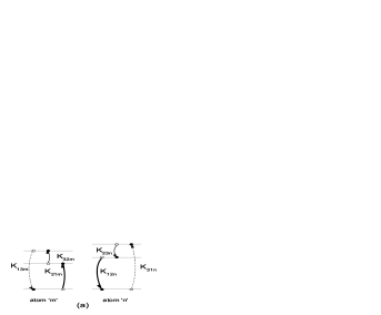
Figure 1: (a) Dipole-dipole transitions between atoms of type $m$ and $n$. (b) Pictorial representation of a highest weight state for atoms of type $m$.

We discuss now the meaning of the labels that characterize the SU(3) irreps (the set $(\Lambda_{m}^{1},\Lambda_{m}^{2})$ and $n_{m}$, or $[k_{1m},k_{2m},k_{3m}]$). Without loss of generality, we can consider $k_{1m}=\Omega_{m}$ ($\Omega_{m}-k_{1m}$ is the number of atoms without any particle in their levels, which are completely decoupled of the rest and do not contribute to the $r_{m}$ eigenvalues). The atoms of each type can be classified according to the number of particle in their levels: (a) unblocked atoms are those with only a particle in their levels. These atoms have all the dipole transition allowed. (b) semi-blocked atoms are those with two particles in their levels, the dipole transitions between the occupied levels are forbidden by Pauli blocking. (c) blocked atoms are those with all their levels occupied, these atoms have all the dipole transitions forbidden, and interact with the others only by the monopole interaction. The Dynkin labels of the irreps determine the number of atoms of each type in the previous situations: $\Lambda_{m}^{1}=k_{1m}-k_{2m}\leq\Omega_{m}$ indicates the number of type-$m$ unblocked atoms, $\Lambda_{m}^{2}=k_{2m}-k_{3m}$ is the number of semi-blocked atoms of type $m$, and the value $k_{3m}$ indicates the number of blocked atoms of type $m$. A representation of a highest weight state is depicted in figure 1. The case where all the atoms are in a unblocked situation corresponds to $\Lambda_{m}^{1}=\Omega_{m}$, $\Lambda_{m}^{2}=0$ and $k_{3m}=0$. Note that integrals of motion (35) guarantee that the total populations (irrespective on the type of atom) in each level ($N_{\alpha},\ \alpha=1,2,3$) are conserved quantities. The number of parameters $E_{k}$ and $\omega_{l}$ in the Richardson-Bethe equations (49) has a simple meaning: the number of $E_{k}$‘s ($M_{1}$) is equal to the number of atoms (of any type) with the first level unoccupied, whereas the number of $\omega_{l}$‘s ($M_{2}$) is the overall number of unblocked and semi-blocked atoms with the third level occupied.

4.2 Particle-particle representation

Another possible realization of the SU(3) algebra is:

$$\mathbf{K}_{21m}=\mathbf{c}_{\downarrow m}^{\dagger}\mathbf{c}_{0m}^{\dagger}\qquad \mathbf{K}_{12m}=\mathbf{c}_{0m}\mathbf{c}_{\downarrow m}\qquad \mathbf{K}_{11m}=1-\mathbf{n}_{0m}$$

$$\mathbf{K}_{31m}=\mathbf{c}_{\uparrow m}^{\dagger}\mathbf{c}_{0m}^{\dagger}\qquad \mathbf{K}_{13m}=\mathbf{c}_{0m}\mathbf{c}_{\uparrow m}\qquad \mathbf{K}_{22m}=\mathbf{n}_{\downarrow m}$$

$$\mathbf{K}_{32m}=\mathbf{c}_{\uparrow m}^{\dagger}\mathbf{c}_{\downarrow m}\qquad \mathbf{K}_{23m}=\mathbf{c}_{\downarrow m}^{\dagger}\mathbf{c}_{\uparrow m}\qquad \mathbf{K}_{33m}=\mathbf{n}_{\uparrow m},$$ (51)

where $\mathbf{c}_{\sigma m}^{\dagger}$ and $\mathbf{c}_{\sigma m}$ are, respectively, fermionic creation and annihilation operators, and $\mathbf{n}_{\sigma m}$ are the number operators $\mathbf{c}_{\sigma m}^{\dagger}\mathbf{c}_{\sigma m}$. The two lowering operators $\mathbf{K}_{21}$ and $\mathbf{K}_{31}$ create a pair of particles and thus form a spinorial pair:

$$\mathbf{P}_{m}=\left(\begin{array}[]{c}\mathbf{P}_{\uparrow m}^{\dagger}\\ \\ \mathbf{P}_{\downarrow m}^{\dagger}\\ \end{array}\right)\equiv\left(\begin{array}[]{c}\mathbf{K}_{31m}\\ \\ \mathbf{K}_{21m}\end{array}\right).$$ (52)

The other lowering operator ($\mathbf{K}_{32m}\equiv\mathbf{T}_{+m}$) is the ladder operator of a $SU_{T}(2)$ subalgebra of SU(3):

$$[\mathbf{T}_{+m},\mathbf{P}_{\downarrow m}^{\dagger}]=\mathbf{P}_{\uparrow m}^{\dagger}.$$ (53)

It is well known that the particle-particle representation of the RG models associated with the SU(2) algebra describes the interaction between scalar pairs [12], whereas the SO(5) version describes the vectorial pairing, i.e., the interaction between pairs forming a triplet [15]. The SU(3) version presented here is associated with an interaction between pairs forming a doublet, we call it spinorial pairing or $T=1/2$ pairing. As it was done in [15] for the SO(5) algebra, from a linear combination of the rational integrals of motion (33), the following pairing Hamiltonian for spinorial pairs results:

$$\mathbf{H}_{T=1/2}=\sum_{m}z_{m}\left(\mathbf{n}_{\uparrow m}+\mathbf{n}_{\downarrow m}\right)+g\sum_{mn}\mathbf{P}_{m}^{\dagger}\cdot\mathbf{P}_{n},$$ (54)

where the scalar product is $\sum_{\sigma=\uparrow\downarrow}\mathbf{P}_{\sigma m}^{\dagger}\mathbf{P}_{\sigma n}$, and we have fixed the parameters $\xi^{1}=1/g$ and $\xi^{2}=0$. In this particle-particle representation of the SU(3) algebra, the Dynkin labels of the highest weight states are associated with the number of unpaired particles in each single particle level $m$ and their transformation properties under the subgroup $SU_{T}(2)$. The number of variables $E_{k}$ and $\omega_{l}$ is, respectively, the number of pairs and the number of $\uparrow$-particles in those pairs.

4.3 Tavis-Cummings models for three level systems and two bosons

In this section we derive another integrable model, which consists of $L$ copies of the SU(3) algebra interacting with two different bosons. This model is derived from the trigonometric version of the previous section in two steps: first we take the bosonic mapping of one copy of the SU(3) algebra (let us say the copy $0$), and then we let the degeneracy $\Omega_{0}$ of this bosonized copy go to infinite.

We assume the SU(3) irrep $(\Lambda_{0}^{1},\Lambda_{0}^{2})=(\Omega_{0},0)$ for the copy to be bosonized. In this case the bosonic mapping for the SU(3) algebra is [23]:

$$\mathbf{K}_{11}\rightarrow\Omega_{0}-\mathbf{a}^{\dagger}\mathbf{a}-\mathbf{b}^{\dagger}\mathbf{b}\qquad \mathbf{K}_{22}\rightarrow\mathbf{a}^{\dagger}\mathbf{a}\qquad \mathbf{K}_{33}\rightarrow\mathbf{b}^{\dagger}\mathbf{b}$$ (55)

$$\mathbf{K}_{31}\rightarrow\mathbf{b}^{\dagger}\sqrt{\Omega_{0}-\mathbf{a}^{\dagger}\mathbf{a}-\mathbf{b}^{\dagger}\mathbf{b}}\qquad \mathbf{K}_{32}\rightarrow\mathbf{b}^{\dagger}\mathbf{a}\qquad \mathbf{K}_{21}\rightarrow\mathbf{a}^{\dagger}\sqrt{\Omega_{0}-\mathbf{a}^{\dagger}\mathbf{a}-\mathbf{b}^{\dagger}\mathbf{b}},$$

where $\mathbf{a}^{\dagger}$ and $\mathbf{b}^{\dagger}$ are boson operators. This mapping is hermitic, therefore the mapping of the operators $\mathbf{K}_{\alpha\beta}$ with $\beta>\alpha$ can be obtained by conjugating the previous ones. In the limit $\Omega_{0}\rightarrow\infty$ the previous mapping is reduced to:

$$\mathbf{K}_{11}\rightarrow\Omega_{0}-\mathbf{a}^{\dagger}\mathbf{a}-\mathbf{b}^{\dagger}\mathbf{b}\qquad \mathbf{K}_{22}\rightarrow\mathbf{a}^{\dagger}\mathbf{a}\qquad \mathbf{K}_{33}\rightarrow\mathbf{b}^{\dagger}\mathbf{b}$$

$$\mathbf{K}_{31}\rightarrow\mathbf{i}\sqrt{\Omega_{0}}\mathbf{b}^{\dagger}\qquad \mathbf{K}_{32}\rightarrow\mathbf{b}^{\dagger}\mathbf{a}\qquad \mathbf{K}_{21}\rightarrow\mathbf{i}\sqrt{\Omega_{0}}\mathbf{a}^{\dagger},$$ (56)

where the imaginary factor $\mathbf{i}$ is introduced for future convenience. We consider now the trigonometric integrals of the RG model (3.1) for a system of $L+1$ copies of the Lie Algebra: $m=0,1,...,L$. Then we bosonize the copy with the ”0” label using (56). In order to avoid divergences in taking the limit $\Omega_{0}\rightarrow\infty$, we define a new set of variables $\epsilon_{m}$ by using the freedom we have to choose the parameters $z_{m}$. These new variables are defined through:

$$\cot(z_{m}-z_{0})=\frac{\epsilon_{m}}{\sqrt{\Omega_{0}}}\qquad m=1,...,L$$ (57)

From this definition and the trigonometric identity ($\cot(A-B)=(\cot(A)\cot(B)+1)/(\cot(B)-\cot(A))$, it is easy to show that in the limit $\Omega_{0}\rightarrow\infty$:

$$\cot(z_{m}-z_{n})\rightarrow\frac{\sqrt{\Omega_{0}}}{\epsilon_{n}-\epsilon_{m}}.$$ (58)

By substituting these results in the trigonometric integrals $\mathbf{R}_{0}$ and $\mathbf{R}_{m}$(3.1), we obtain:

$$\hat{\mathcal{R}}_{0}= -\zeta^{1}\mathbf{a}^{\dagger}\mathbf{a}-(\zeta^{1}+\zeta^{2})\mathbf{b}^{\dagger}\mathbf{b}+\mathcal{C}_{0}\mathbf{1}$$ (59)

$$+\sum_{n=1}^{L}\left(\mathbf{a}^{\dagger}\mathbf{K}_{12n}+\mathbf{a}\mathbf{K}_{21n}+\mathbf{b}\mathbf{K}_{31n}+\mathbf{b}^{\dagger}\mathbf{K}_{13n}+\epsilon_{n}\mathbf{K}_{11n}\right)$$

$$\hat{\mathcal{R}}_{m}= -\zeta^{1}\mathbf{K}_{22m}-(\zeta^{1}+\zeta^{2})\mathbf{K}_{33m}+\mathcal{C}_{m}\mathbf{1}+\sum_{n(n\neq m)}^{L}\frac{\sum_{\alpha\beta}\mathbf{K}_{\alpha\beta m}\mathbf{K}_{\beta\alpha n}}{\epsilon_{m}-\epsilon_{n}}$$

$$-\left(\mathbf{a}^{\dagger}\mathbf{K}_{12m}+\mathbf{a}\mathbf{K}_{21m}+\mathbf{b}\mathbf{K}_{31m}+\mathbf{b}^{\dagger}\mathbf{K}_{13m}+\epsilon_{m}\mathbf{K}_{11m}\right),$$

where we have rescaled the operators $\mathbf{R}_{0}$ and $\mathbf{R}_{m}$ ($\hat{\mathcal{R}}_{0}$ $\equiv$ $\mathbf{R}_{0}/\sqrt{\Omega_{0}}$ and $\hat{\mathcal{R}}_{m}$ $\equiv$ $\mathbf{R}_{m}/\sqrt{\Omega_{0}}$), dropped the terms with inverse powers of $\sqrt{\Omega_{0}}$, and defined new variables:

$$\zeta^{a}=\frac{\xi^{a}}{\sqrt{\Omega_{0}}}.$$ (60)

The constants in the integrals of motion (59) are $\mathcal{C}_{0}=-(1/3)\sum_{l}\epsilon_{l}n_{l}+(2\zeta^{1}+\zeta^{2})(\Omega_{0}/3)$ and $\mathcal{C}_{m}=(\epsilon_{m}n_{m})/3+\sum_{l}^{\prime}n_{l}/(\epsilon_{l}-\epsilon_{m})+(2\zeta^{1}+\zeta^{2})n_{m}/3$.

To obtain the eigenvalues of the previous operators, we take the eigenvalues (46), with $Z(z_{j}-z_{i})$ and $Z(E_{k}-z_{i})$ substituted by cotangent functions, and then the limit $\Omega_{0}\rightarrow\infty$. Before performing this limit we introduce, as we did in (57), two new sets of variables associated with the parameters $E_{k}$ and $\omega_{k}$:

$$\cot(z_{0}-E_{k})=-\frac{x_{k}}{\sqrt{\Omega_{0}}}\qquad\cot(z_{0}-\omega_{l})=-\frac{y_{l}}{\sqrt{\Omega_{0}}}.$$ (61)

The same trigonometric identity that yields (58) allows us to write the limit $\Omega_{0}\rightarrow\infty$ of the following functions:

$$\cot(z_{m}-E_{k})\rightarrow\frac{\sqrt{\Omega_{0}}}{x_{k}-\epsilon_{m}}\qquad\cot(z_{m}-\omega_{l})\rightarrow\frac{\sqrt{\Omega_{0}}}{y_{l}-\epsilon_{m}}\qquad\cot(\omega_{l^{\prime}}-\omega_{l})\rightarrow\frac{\sqrt{\Omega_{0}}}{y_{l}-y_{l^{\prime}}}$$

$$\cot(E_{k}-E_{l})\rightarrow\frac{\sqrt{\Omega_{0}}}{x_{l}-x_{k}}\qquad\cot(E_{k}-\omega_{l})\rightarrow\frac{\sqrt{\Omega_{0}}}{y_{l}-x_{k}},$$ (62)

where we have used the definition (57). With the limit values of the previous cotangent functions, the eigenvalues (46) become:

$$\mathrm{r}_{0}= \sum_{n=1}^{L}k_{1n}\epsilon_{n}+\mathcal{C}_{0}-\sum_{k=1}^{M_{1}}x_{k}$$ (63)

$$\mathrm{r}_{m}= -\zeta^{1}k_{2m}-(\zeta^{1}+\zeta^{2})k_{3m}+\mathcal{C}_{m}+\sum_{n=1(n\neq m)}^{L}\frac{\sum_{\alpha=1}^{3}k_{\alpha m}k_{\alpha n}}{\epsilon_{m}-\epsilon_{n}}-k_{1m}\epsilon_{m}$$ (64)

$$+(k_{1m}-k_{2m})\sum_{k=1}^{M_{1}}\frac{1}{x_{k}-\epsilon_{m}}+(k_{2m}-k_{3m})\sum_{l=1}^{M_{2}}\frac{1}{y_{l}-\epsilon_{m}},$$

which are the eigenvalues of the operators (59). Note that the term $\mathcal{C}_{0}$, that diverges in the limit $\Omega_{0}\rightarrow\infty$, appears explicitly both in the operator and its eigenvalue, then we can easily get rid of it. $\epsilon_{m}$ are free parameters and the variables $x_{k}$ and $y_{l}$ are solutions of the Richardson-Bethe equations in the limit $\Omega_{0}\rightarrow\infty$. To derive them, we consider the Richardson-Bethe equations in the trigonometric case, which can be read from equations (3.4) and (3.4) with $Z$ substituted by cotangent functions. Then, using (62) we obtain:

$$\sum_{k^{\prime}(k^{\prime}\neq k)}^{M_{1}}\frac{2}{x_{k^{\prime}}-x_{k}}-\sum_{l=1}^{M_{2}}\frac{1}{y_{l}-x_{k}}-\sum_{m=1}^{L}\frac{k_{1m}-k_{2m}}{\epsilon_{m}-x_{k}}-x_{k}=-\zeta^{1}\quad (k=1,..,M_{1})$$

$$-\sum_{k=1}^{M_{1}}\frac{1}{x_{k}-y_{l}}+\sum_{l^{\prime}(l^{\prime}\neq l)}^{M_{2}}\frac{2}{y_{l^{\prime}}-y_{l}}-\sum_{m=1}^{L}\frac{k_{2m}-k_{3m}}{\epsilon_{m}-\omega_{l}}=-\zeta^{2}\quad (l=1,..,M_{2}).$$ (65)

Note that the resulting Richardson-Bethe equations are identical to those in the rational case except by the linear term in the first line. The integrals of motion (35) are now:

$$\mathbf{N}_{3}=\sum_{m=1}^{L}\mathbf{K}_{33m}+\mathbf{n}_{b}\qquad\mathbf{N}_{2}=\sum_{m=1}^{L}\mathbf{K}_{22m}+\mathbf{n}_{a}$$

$$\mathbf{N}_{1}=\sum_{m=1}^{L}\mathbf{K}_{11m}+\Omega_{0}-\mathbf{n}_{a}-\mathbf{n}_{b}.$$ (66)

The physical meaning of the Dynking labels $(\Lambda_{m}^{1},\Lambda_{m}^{2})$ and $n_{m}$ is not modified by the introduction of the bosons, and it is the same already discussed above. The number of parameters $x_{k}$ and $y_{l}$ ($M_{1}$ and $M_{2}$) in the Richardson-Bethe equations (65) can be obtained from the general formula (49), by extending the sum to the bosonized copy, and noting that the Young labels associated with it are $[k_{10},k_{20},k_{30}]=[\Omega_{0},0,0]$.

One of the simplest Hamiltonian that can be derived from the previous integrals of motion, is obtained by considering just one non-bosonized copy of the SU(3) algebra. Therefore $L=1$ and we have 2 integrals of motion: $\mathbf{R}_{0}$ and $\mathbf{R}_{1}$. By taking a linear combination of these integrals we arrive to:

$$\mathbf{H} = z_{0}\left(\hat{\mathcal{R}}_{0}-\mathcal{C}_{0}\mathbf{1}\right)+z_{1}\left(\hat{\mathcal{R}}_{1}-\mathcal{C}_{1}\mathbf{1}\right)$$ (67)

$$= \omega_{a}\mathbf{n}_{a}+\omega_{b}\mathbf{n}_{b}+\eta_{2}\mathbf{K}_{22}+\eta_{3}\mathbf{K}_{33}+g\left(\mathbf{a}^{\dagger}\mathbf{K}_{12}+\mathbf{a}\mathbf{K}_{21}+\mathbf{b}\mathbf{K}_{31}+\mathbf{b}^{\dagger}\mathbf{K}_{13}\right),$$

where $\mathbf{K}_{\alpha\beta}$ are the generators of the non-bosonized copy. The parameters of the Hamiltonian are related to the RG parameters by:

$$\zeta^{1}=\frac{\omega_{a}(\Delta_{\eta}-\Delta_{\omega})}{g\Delta_{\omega}}\qquad\zeta^{2}=\frac{\Delta_{\eta}-\Delta_{\omega}}{g}\qquad\epsilon_{1}=\frac{\omega_{a}\Delta_{\eta}-\Delta_{\omega}\eta_{2}}{g\Delta_{\omega}},$$ (68)

and the constants $z_{0}$ and $z_{1}$ are:

$$z_{0}=-g\frac{\Delta_{\omega}}{\Delta_{\eta}-\Delta_{\omega}}\qquad z_{1}=-g\frac{\Delta_{\eta}}{\Delta_{\eta}-\Delta_{\omega}},$$ (69)

with $\Delta_{\omega}\equiv\omega_{b}-\omega_{a}$, and $\Delta_{\eta}\equiv\eta_{3}-\eta_{2}$. The previous Hamiltonian describes the interaction between a set of $\Omega_{1}$ identical three level atoms and two modes of the electric field in the so called Rotating-Wave-Approximation [17], and is a generalized version of the Tavis-Cummings model for three level atoms.

If we write the Hamiltonian (67) in the particle-particle representation, we obtain the interaction between a doublet of pairs and a doublet of bosons:

$$\mathbf{H}=\omega_{+}\mathbf{n}_{+}+\omega_{-}\mathbf{n}_{-}+\epsilon_{\uparrow}\mathbf{n}_{\uparrow}+\epsilon_{\downarrow}\mathbf{n}_{\downarrow}+g\left(\mathbf{P}^{\dagger}\cdot\mathbf{b}+\mathbf{P}\cdot\mathbf{b}^{\dagger}\ \right),$$ (70)

where we have redefined the bosons $\mathbf{a}^{\dagger}\rightarrow\mathbf{b}_{-}^{\dagger}$, $\mathbf{b}^{\dagger}\rightarrow\mathbf{b}_{+}^{\dagger}$, and the scalar product, $\mathbf{P}^{\dagger}\cdot\mathbf{b}$, is $\mathbf{P}^{\dagger}_{\uparrow}\mathbf{b}_{+}+\mathbf{P}^{\dagger}_{\downarrow}\mathbf{b}_{-}$. More complex Hamiltonians can be derived from the integrals (59), but we will not discuss them here.

5 Conclusions

In this contribution we introduced a Gaudin algebra valid for any simple Lie algebra in the rational, trigonometric, and hyperbolic cases. With this algebra, we derived the complete set of quadratic RG integrals of motion, and found their respective eigenvalues. Focusing this formalism on the rank-two SU(3) algebra, we worked out in detail the RG models. For the rational case, expressions for the integrals of motion of degree three were obtained, and it was verified that their number is the necessary to match the number of integrals of motion with the number of degrees of freedom of the quantum model. Some physical applications of the SU(3) models were discussed. The physical meaning of the variables in the RG formalism were discussed for two different representations of the SU(3) algebra, namely, the particle-hole representation and the particle-particle one. By taking the trigonometric version of the models, we derived a new family of integrable models which are related to a generalization of the Tavis-Cummings model to three level atoms and two bosons. It was out of the scope of this contribution to explore all the possible physical applications of the SU(3) RG models, some examples were given and others are expected to come. We think that we have put the ground for more detailed studies, such as numerical studies of the solutions and comparison with approximative techniques in physical scenarios beyond the limits of traditional diagonalization methods. The formalism presented here can be easily applied to other Lie algebras. Some physically relevant examples are the SU(4) and SO(5) versions in the description of High temperature superconductors [24], the SO(8) version for isovector-isoscalar pairing [25], and the SU(n) versions which include generalized Tavis-Cummings models for $n$-levels atoms interacting with $n-1$ different bosonic modes. The formalism can likewise be extended to the elliptic RG models, where no linear term in the quadratic integrals of motion is allowed. Another interesting extension of the present contribution is to derive more general solutions to the Gaudin conditions (10), using the very well studied solutions to the Classical Yang-Baxter Equations [26]. Finally, the higher rank RG models can be useful to shed some light in the non completely well established definition of number of degrees of freedom in finite Quantum systems. In this contribution, the definition of integrability coming from the Yang-Baxter Equation was linked to the one coming from the equality between the number of quantum degrees of freedom and the number of independent integrals of motion. This latter definition, initially supposed to be exclusively related to dynamical symmetric models, can be extended, as shown in this contribution, to the RG models, which are not necessarily dynamical symmetric.

References

References

- [1] Dukelsky J, Pittel S and Sierra G 2004 Rev. Mod. Phys. 76 643
- [2] Links J, Zhou H-Q, McKenzie R H and Gould M D 2003 J. Phys. A 36 R63-R104
- [3] Richardson R W 1963 Phys. Lett. 3 277; Richardson R W 1966 Phys. Rev. 141 949
- [4] Gaudin M 1976 J. Phys. (Paris) 37 1087
- [5] von Delft J and Poghossian R 2002 Phys. Rev. B 66 134502
- [6] Jurco B 1989 J. Math. Phys. 30 1289
- [7] Guan X-W, Foerster A, Links J and Zhou H-Q 2002 Nucl. Phys. B 642 501
- [8] Asorey M, Falceto F and Sierra G 2002 Nucl. Phys. B 622 593
- [9] Ushveridze A G 1994 Quasi-exactly solvable models in quantum mechanics (Bristol: Institute of Physics) p 357
- [10] Ortiz G, Somma R, Dukelsky J and Rombouts S 2005 Nucl. Phys. B 707 421
- [11] Amico L, Di Lorenzo A and Osterloch A 2001 Phys. Rev. Lett. 86 5759
- [12] Dukelsky J, Esebbag C and Schuck P 2001 Phys. Rev. Lett. 87 066403
- [13] Dukelsky J, Dussel G G, Esebbag C and Pittel S 2004 Phys. Rev. Lett. 93 050403
- [14] Links J, Zhou H-Q, Gould M D and McKenzie R H 2002 J. Phys. A 35 6459
- [15] Dukelsky J, Gueorguiev V, Van Isacker P, Dimitrova S, Errea B and Lerma H S 2006 Phys. Rev. Lett. 96 072503
- [16] Lerma H S, Errea B, Dukelsky J, Pittel S and Van Isacker P 2006 Phys. Rev C 74 024314
- [17] Yoo H I and Eberly J H 1985 Phys. Rep. 118 239
- [18] Chervov A, Rybnikov L and Talalaev D 2004 Rational Lax operators and their quantization Preprint hep-th/0404106
- [19] Talalaev D 2006 Funct. Anal. Appl. 40 73
- [20] Zhang W M and Feng D H 1995 Phys. Rep. 252 1
- [21] Di Francesco P, Mathieu P and Sénéchal D 1997 Conformal Field Theory (New York: Springer) p 489
- [22] Wybourne B G 1974 Classical Groups for Physicists (New York: Wiley-Interscience)
- [23] Klein A and Marshalek E R 1991 Rev. Mod. Phys. 63 2
- [24] Guidry M, Wu L-A, Sun Y and Wu C-L 2001 Phys. Rev. B 63 134516
- [25] Evans J A, Dussel G G, Maqueda E E and Perazzo P J 1981 Nucl. Phys. A 367 77
- [26] Belavin A A and Drinfel’d V G 1982 Funct. Anal. Appl. 16 159