An ultradiscrete matrix version of the fourth Painlevé equation

Abstract

We establish a matrix generalization of the ultradiscrete fourth Painlevé equation ($\mathrm{ud}$-$\mathrm{P}_{\mathrm{IV}}$). Well-defined multicomponent systems that permit ultradiscretization are obtained using an approach that relies on a group defined by constraints imposed by the requirement of a consistent evolution of the systems. The ultradiscrete limit of these systems yields coupled multicomponent ultradiscrete systems that generalize $\mathrm{ud}$-$\mathrm{P}_{\mathrm{IV}}$. The dynamics, irreducibility, and integrability of the matrix valued ultradiscrete systems are studied.

${\dagger}$ cmfield@maths.usyd.edu.au      ${\ddagger}$ chriso@maths.usyd.edu.au

1 Introduction

Discrete Painlevé equations are difference equation analogs of classical Painlevé equations [17] and have been extensively studied recently (see the review article [6]). The ultradiscrete Painlevé equations are discrete equations considered to be extended cellular automata (they may also be considered as piecewise linear systems) that are derived by applying the ultradiscretization process [24] to discrete Painlevé equations. This process has been accepted as one that preserves integrability [7]. Particular indicators of integrability in the ultradiscrete setting include the existence of a Lax pair [19], an analog of singularity confinement [9], and special solutions [16].

All of the preceding examples arising from ultradiscretization are one-component (that is, scalar) systems. Generalizations of integrable systems to associative algebras have been considered for many years (see [15], and references therein). However, the general methods and results previously obtained are inapplicable in the ultradiscrete setting, due to the requirement of a subtraction free setting. We present for the first time a matrix generalization of an ultradiscrete system.

The constraints related to the subtraction free setting and consistent evolution are studied in a group theoretic approach, in which one may also describe the nature of the irreducible subsystems. As an application of this method, we introduce a matrix version of the $\mathrm{ud}$-$\mathrm{P}_{\mathrm{IV}}$ of [11] which is derived by applying the ultradiscretization procedure to $q$-$\mathrm{P}_{\mathrm{IV}}$,

$$\begin{array}[]{c c c}f_{0}(qt)&=&a_{0}a_{1}f_{1}(t)\frac{1+a_{2}f_{2}(t)+a_{2}a_{0}f_{2}(t)f_{0}(t)}{1+a_{0}f_{0}(t)+a_{0}a_{1}f_{0}(t)f_{1}(t)}\\ f_{1}(qt)&=&a_{1}a_{2}f_{2}(t)\frac{1+a_{0}f_{0}(t)+a_{0}a_{1}f_{0}(t)f_{1}(t)}{1+a_{1}f_{1}(t)+a_{1}a_{2}f_{1}(t)f_{2}(t)}\\ f_{2}(qt)&=&a_{1}a_{2}f_{0}(t)\frac{1+a_{1}f_{1}(t)+a_{1}a_{2}f_{1}(t)f_{2}(t)}{1+a_{2}f_{2}(t)+a_{0}a_{2}f_{0}(t)f_{2}(t)}.\end{array}$$ (1.1)

With the explicit form of the matrices derived, the new systems can be considered as coupled multicomponent generalizations. It should be stressed that the approach of this paper gives all possible ultradiscretizable matrix valued versions of (1.1).

The reason for choosing $q$-$\mathrm{P}_{\mathrm{IV}}$ is that it has already been thoroughly and expertly investigated in the scalar case (i.e., when $f_{i}$ and $a_{i}$ are scalar) [11]. In [11], $q$-$\mathrm{P}_{\mathrm{IV}}$ was shown to admit the action of the affine Weyl group of type $A_{2}^{(1)}$ as a group of Bäcklund transformations, to have classical solutions expressible in terms of $q$-Hermite-Weber functions, to have rational solutions, and its connection with the classification of Sakai [23] was also investigated. Furthermore, the ultradiscrete limit was taken in [11], and was shown to also admit affine Weyl group representations. As $q$-$\mathrm{P}_{\mathrm{IV}}$ is such a rich system, and has already been well-studied, this makes it a perfect system for the application of our approach of ultradiscrete matrix generalization.

Before turning to the derivation of matrix $\mathrm{ud}$-$\mathrm{P}_{\mathrm{IV}}$, ultradiscretization should be introduced in more detail, so that the reason for certain constraints given later will be clear.

The process is a way of bringing a rational expression, $f$, in variables (or parameters) $a_{1},\ldots,a_{n}$ to a new expression, $F$, in new ultradiscrete variables $A_{1},\ldots,A_{n}$, that are related to the old variables via the relation $a_{i}=e^{A_{i}/\epsilon}$ and limiting process

$$F(A_{1},\ldots,A_{n})=\lim_{\epsilon\to 0}\epsilon\log f(a_{1},\ldots,a_{n}).$$ (1.2)

In general it is sufficient to make the following correspondences between binary operations

$$\begin{array}[]{c c c}a+b&\to&\max(A,B)\\ ab&\to&A+B\\ a/b&\to&A-B.\end{array}$$ (1.3)

This process is a way in which we may take an integrable mapping over the positive real numbers $\mathbb{R}^{+}$ to an integrable mapping over the max-plus semiring [5]. The requirement that the pre-ultradiscrete equations are subtraction free expressions of a definite sign is a more stringent restraint in the matrix setting than the one-component setting, and it is this requirement which motivates the particular form of our matrix system.

The outline of this paper is as follows. In section 2, a $q$-$\mathrm{P}_{\mathrm{IV}}$ is derived in the noncommutative setting, where the dependent variables take their values in an associative algebra. In section 3 conditions on the matrix forms of the dependent variables and parameters of $q$-$\mathrm{P}_{\mathrm{IV}}$ are derived such that it has a well-defined evolution and is ultradiscretizable. The group theoretic approach is adopted to describe the constraints on the system. In section 4 the ultradiscrete version of this system is derived, and some of the rich phenomenology of the derived matrix valued ultradiscrete $\mathrm{P}_{\mathrm{IV}}$ is displayed and analyzed in section 5.

2 Symmetric $q$-$\mathrm{P}_{\mathrm{IV}}$ on an associative algebra

In this section it is shown that the symmetric $q$-$\mathrm{P}_{\mathrm{IV}}$ of [11] can be derived from a Lax formalism in the noncommutative setting, where the dependent variables $\{f_{i}\}$ take values in an a priori arbitrary associative algebra, $\mathcal{A}$, with unit $I$ over a field $\mathbb{K}$ (when we turn to ultradiscretization, the requirement of a field will be modified, but not in such a way as to affect the derivation from a Lax pair). This puts the present work in the context of other recent work on integrable systems such as [14] and [15] where the structure of integrable ODEs and PDEs (respectively) was extended to the domain of associative algebras, and [1] where Painlevé equations were defined on an associative algebra (see also [15]). This trend has also been present in work on discrete integrable systems, such as [2] where the higher dimensional consistency (consistency around a cube) property was investigated for integrable partial difference equations defined on an associative algebra, and [4] where an initial value problem on the lattice KdV with dependent variables taking values in an associative algebra was studied, leading to exact solutions.

The auxiliary (spectral) parameter $x$, time variable $t$ and constant $q$ belong to the field $\mathbb{K}$. The dependent variables $\{f_{i}\}\in\mathcal{A}$, system parameters $\{b_{i}\}\in\mathcal{A}$ ($i\in\{0,1,2\}$), and we define

$$\Gamma_{i}:=I+b^{3}_{i}f_{i}+b^{3}_{i}b^{3}_{i+1}f_{i}f_{i+1},$$ (2.1)

up to an arbitrary ordering of the $b_{j}^{3}$ and $f_{j}$ factors. (It will be shown that the ordering of these factors within $\Gamma_{i}$ is of no consequence for either the integrability of the system or the existence of a well defined evolution in the ultradiscrete limit.) The invertibility of these expressions is assumed, that is $\Gamma_{i}^{-1}\in\mathcal{A}$.

We derive the system from a linear problem to settle other ordering issues in the noncommutative setting. The $q$-type Lax formalism is given by

$$\phi(qx,t)=L(x,t)\phi(x,t)\quad,\quad\phi(x,qt)=M(x,t)\phi(x,t)$$ (2.2)

where

$$L(x,t)\ =\ \left(\begin{array}[]{ccc}(1+x^{2})I&b_{0}f_{0}t^{-\frac{2}{3}}&0\\ 0&(1+x^{2})I&b_{1}f_{1}t^{-\frac{2}{3}}\\ b_{2}f_{2}t^{-\frac{2}{3}}&0&(1+x^{2})I\end{array}\right)\$$ (2.3d)

$$M(x,t)\ =\ \left(\begin{array}[]{ccc}0&b_{2}^{-2}\,\Gamma_{2}&0\\ 0&0&b_{0}^{-2}\,\Gamma_{0}\\ b_{1}^{-2}\,\Gamma_{1}&0&0\end{array}\right).$$ (2.3h)

The ultradiscrete version of this linear problem (for the usual commutative case) originally appeared in [10].

The compatibility condition for this linear problem reads

$$M(qx,t)L(x,t)=L(x,qt)M(x,t),$$ (2.3d)

and leads to

$$\begin{array}[]{c c c}b_{0}\,\overline{f}_{0}&=&q^{2/3}\,b_{2}^{-2}\>\Gamma_{2}\,b_{1}\,f_{1}\,\Gamma_{0}^{-1}\,b_{0}^{2},\\ b_{1}\,\overline{f}_{1}&=&q^{2/3}\,b_{0}^{-2}\>\Gamma_{0}\,b_{2}\,f_{2}\,\Gamma_{1}^{-1}\,b_{1}^{2},\\ b_{2}\,\overline{f}_{2}&=&q^{2/3}\,b_{1}^{-2}\>\Gamma_{1}\,b_{0}\,f_{0}\,\Gamma_{2}^{-1}\,b_{2}^{2},\end{array}$$ (2.3e)

where the overline denotes a time-update and $\overline{b}_{i}=b_{i}$.

Following [11], we show a product of the dependent variables can be regarded as the independent variable. With $\{f^{-1}_{i}\}\in\mathcal{A}$, $\{b^{-1}_{i}\}\in\mathcal{A}$ (i.e., we are working with a skew field) and specifying that the product $b_{0}f_{0}b_{1}f_{1}b_{2}f_{2}$ is proportional to $I$, it is seen that $b_{0}f_{0}b_{1}f_{1}b_{2}f_{2}=qc^{2}I$ where $c\in\mathbb{K}$ and $\overline{c}=qc$. Without loss of generality we set $c=t$. From now on

$$b_{0}f_{0}b_{1}f_{1}b_{2}f_{2}=qt^{2}I$$ (2.3f)

will be imposed (so the algebra generated by all three $\{f_{i}\}$ and $I$ is not free). The invertibility of the algebra elements $\{f_{i}\}$ and $\{b_{i}\}$ is a consequence of the explicit matrix representation of these objects for the well-defined matrix systems studied in the next sections.

With the restriction

$$b_{0}^{3}\,b_{1}^{3}\,b_{2}^{3}=qI$$ (2.3g)

imposed, the map (2.3e) is a noncommuting generalization of $q$-$\mathrm{P}_{\mathrm{IV}}$. If we specify that $b_{i}$ and $f_{i}$ be matrix valued, the only requirement for a consistent evolution is that the $\Gamma_{i}$ are invertible. This however is too general a system to be ultradiscretized, since in general we require the inverse to be subtraction free.

If all variables commute, then after the change of variables $a_{i}:=b_{i}^{3}$ the map reduces to $q$-$\mathrm{P}_{\mathrm{IV}}$, (1.1), as presented in [11].

3 Ultradiscretizable matrix structure

The conditions (2.3f) and (2.3g) can be used in conjunction with (2.3e) to define constraints that lead to a consistent evolution on $\mathcal{A}$ as a free algebra with two constant (say $b_{1}$ and $b_{2}$) and two variable (say $f_{1}$ and $f_{2}$) generators. Regarding these as $n\times n$ (or even infinite dimensional) matrices leads to multicomponent systems. However, the aim of the present work is to derive matrix (or multicomponent) ultradiscrete systems, and hence, as we require the expressions to be subtraction free, we have considerably less freedom than this general setting.

Due to this restriction, we restrict $\mathcal{A}$ to be the group of invertible non-negative matrices, that is we set

$$\mathcal{A}=S_{n}\ltimes\mathbb{K}^{n}$$ (2.3a)

where $S_{n}$ is the symmetric group and $\mathbb{K}$ will further be restricted to be $\mathbb{R}^{+}$ in models where we wish to perform ultradiscretization. For our purposes $S_{n}$ is realized as $n\times n$ matrices of the form $\delta_{i\sigma(j)}$ for $\sigma\in S_{n}$. (This group decomposition result can been seen in [3].) We define the homomorphism $\pi:\mathcal{A}\to\mathcal{A}/\mathbb{K}^{n}=S_{n}$ to be the homomorphism obtained as a result of the above semidirect product. This allows us to more easily deduce the form of the matrices $\{f_{i}\}$, $\{b_{i}\}$, that give a well-defined evolution.

Since $\mathcal{A}$ is a semidirect product, the elements $b_{i}$ and $f_{i}$ can be uniquely written in the form

$$\begin{array}[]{c c c}b_{i}&=&\beta_{i}\,s_{i}\\ f_{i}(t)&=&\digamma_{i}(t)\,z_{i},\end{array}$$ (2.3b)

where $\pi(b_{i})=s_{i}\in S_{n}$, $\pi(f_{i}(t))=z_{i}\in S_{n}$, and $\beta_{i}$ and $\digamma_{i}(t)$ are diagonal matrices containing the $n$ components of $b_{i}$ and $f_{i}(t)$ respectively (we leave the matrix representation implicit).

We now derive further restrictions on $\{s_{i}\}$ and $\{z_{i}\}$ such that the evolution is consistent, and all terms in the map (such as the $\Gamma_{i}$) remain in $\mathcal{A}$, (2.3a).

Consider the following form of $\Gamma_{i}$,

$$\Gamma_{i}:=I+b^{3}_{i}f_{i}+b^{3}_{i}b^{3}_{i+1}f_{i+1}f_{i}.$$ (2.3c)

As $\pi(I)=I$, $\pi(\Gamma_{i})=I$ and this implies

$$s_{i}^{3}z_{i}=I\qquad i\in\{0,1,2\}.$$ (2.3d)

This is the only condition that arises from the requirement that $\Gamma_{i}\in\mathcal{A}$, where $\mathcal{A}$ is given by (2.3a). It is immediately seen that condition (2.3d) is independent of the ordering of the $b_{i}^{3}f_{i}$ term in $\Gamma_{i}$. There are 24 possible orderings of $b_{i}^{3}b_{i+1}^{3}f_{i+1}f_{i}$ (we do not consider the possibility of splitting up the $b_{i}$ factors, as $b_{i}^{3}=:a_{i}$ is the parameter in the commutative case [11]). Of these 24 possibilities, 8 also require the commutativity of $s_{1}^{3}$ and $s_{j}^{3}$ (equivalently $z_{i}$ and $z_{i+1}$). It is shown in A that these additional commutativity relations do not change the restrictions on $\{s_{i}\}$ and $\{z_{i}\}$. (That is, commutativity of $s_{i}^{3}$ and $s_{j}^{3}$ is a consequence of the full set of relations.)

Requiring the preservation of (2.3b) as the variables evolve, the projection of (2.3e) onto $S_{n}$, with (2.3d), gives

$$s_{i}^{4}=s_{i+1}^{2}s_{i-1}^{2}\qquad i\in\{0,1,2\}.$$ (2.3e)

The projection of the constraints (2.3f) and (2.3g) onto $S_{n}$, with (2.3d), gives

$$s_{2}^{2}s_{1}^{2}s_{0}^{2}=I$$ (2.3f)

and

$$s_{0}^{3}s_{1}^{3}s_{2}^{3}=I$$ (2.3g)

respectively.

Therefore, to give a consistent evolution that permits ultradiscretization, $\{s_{i}\}$ are homomorphic images of the group generators of

$$G=\langle g_{0},g_{1},g_{2}\,|\,g_{0}^{4}=g_{1}^{2}g_{2}^{2},\,g_{1}^{4}=g_{2}^{2}g_{0}^{2},\,g_{2}^{4}=g_{0}^{2}g_{1}^{2},\,g_{2}^{2}g_{1}^{2}g_{0}^{2}=1,\,g_{0}^{3}g_{1}^{3}g_{2}^{3}=1\rangle$$ (2.3h)

in $S_{n}$; $\{z_{i}\}$ are given by (2.3d). The group $G$ has order 108. The order of the generators of $G$ is shown to be 18 in A.

4 Ultradiscretization

We now consider the ultradiscretization of the matrix valued systems derived in the previous section. The components of the ultradiscretized systems belong to the max-plus semiring, $S$, which is the set $\mathbb{R}\cup\{-\infty\}$ adjoined with the binary operations of $\max$ and $+$ (often called tropical addition and tropical multiplication). To map the pre-ultradiscrete expression to the max-plus semiring, we may simply make the correspondences (1.3) on the level of the components. (So $-\infty$ becomes the additive identity and $0$ becomes the multiplicative identity.) By ultradiscretizing matrix operations, we arrive at the following definitions of matrix operations over $S$. If $A=(a_{ij})$ and $B=(b_{ij})$, then following [19], we define tropical matrix addition and multiplication, $\oplus$ and $\otimes$, by the equations

$$(A\oplus B)_{ij}:=\max(a_{ij},b_{ij})$$

$$(A\otimes B)_{ij}:=\max_{k}(a_{ik}+b_{kj})$$

along with a scalar operation given by

$$(\lambda\otimes A)_{ij}:=(\lambda+a_{ij})$$

for all $\lambda\in S$. In the ultradiscrete limit $0$ is mapped to $-\infty$, and $1$ is mapped to $0$; hence the identity matrix, $I$, is the matrix with $0$s along the diagonal and $-\infty$ in every other entry. In the same way it is clear what happens to matrix realizations of members of $S_{n}$ in the ultradiscrete limit.

An ultradiscretized member of the group $\mathcal{A}$, (2.3a), has a decomposition of the form

$$D=\Delta\otimes T$$

(cf. equation (2.3b)) where $\Delta$ has $-\infty$ for all off-diagonal entries and $T$ is an ultradiscretization of an element of $S_{n}$. Its inverse is given by

$$D^{-1}=T^{-1}\otimes\Delta^{-1},$$

where $(\Delta^{-1})_{ii}\equiv-(\Delta)_{ii}$ and all off-diagonal entries are $-\infty$.

As well as the matrix map, the correspondence also allows us to easily write the Lax pair over the semialgebra.

$$\mathcal{L}(X,T)\ =\ \left(\begin{array}[]{ccc}\max(0,2X)\otimes I&B_{0}\otimes F_{0}\otimes-\frac{2T}{3}&-\infty\\ -\infty&\max(0,2X)\otimes I&B_{1}\otimes F_{1}\otimes-\frac{2T}{3}\\ B_{2}\otimes F_{2}\otimes-\frac{2T}{3}&-\infty&\max(0,2X)\otimes I\end{array}\right)\$$ (2.3ad)

$$\ \mathcal{M}(X,T)\ =\ \left(\begin{array}[]{ccc}-\infty&B_{2}^{-2}\,\otimes\,\Gamma_{2}&-\infty\\ -\infty&-\infty&B_{0}^{-2}\,\otimes\,\Gamma_{0}\\ B_{1}^{-2}\,\otimes\,\Gamma_{1}&-\infty&-\infty\end{array}\right).$$ (2.3ah)

Where the ultradiscretization of $\Gamma_{i}$, as given in (2.1), is the matrix

$$\Gamma_{i}=I\oplus\left(B_{i}^{3}\otimes F_{i}^{3}\right)\oplus\left(B_{i}^{3}\otimes B_{i+1}^{3}\otimes F_{i}\otimes F_{i+1}\right).$$ (2.3ab)

The compatibility condition reads

$$\mathcal{M}(X+Q,T)\otimes\mathcal{L}(X,T)=\mathcal{L}(X,T+Q)\otimes\mathcal{M}(X,T),$$ (2.3ac)

and gives the ultradiscrete equation over an associative $S$-algebra

$$\begin{array}[]{c c c}B_{0}\otimes\overline{F}_{0}&=&\frac{2}{3}Q\otimes B_{2}^{-2}\otimes\Gamma_{2}\otimes B_{1}\otimes F_{1}\otimes\Gamma_{0}^{-1}\otimes B_{0}^{2},\\ B_{1}\otimes\overline{F}_{1}&=&\frac{2}{3}Q\otimes B_{0}^{-2}\otimes\Gamma_{0}\otimes B_{2}\otimes F_{2}\otimes\Gamma_{1}^{-1}\otimes B_{1}^{2},\\ B_{2}\otimes\overline{F}_{2}&=&\frac{2}{3}Q\otimes B_{1}^{-2}\otimes\Gamma_{1}\otimes B_{0}\otimes F_{0}\otimes\Gamma_{2}^{-1}\otimes B_{2}^{2}.\end{array}$$ (2.3ad)

The ultradiscrete version of the restrictions (2.3f) and (2.3g) are

$$B_{0}\otimes F_{0}\otimes B_{1}\otimes F_{1}\otimes B_{2}\otimes F_{2}=(Q+2T)\otimes I$$ (2.3ae)

and

$$B_{0}^{3}\otimes B_{1}^{3}\otimes B_{2}^{3}=Q\otimes I.$$ (2.3af)

(Of course, it would have been equally legitimate to apply the correspondence on the level of the map (2.3e) without starting from a derivation from the ultradiscretized Lax pair.)

It is easily seen that if $2Q/3$, the parameter $T$, and all components of the map belong to $\mathbb{Z}$ then at all time-steps all components (not formally equal to $-\infty$) belong to $\mathbb{Z}$. It is this property which motivates the term ‘extended cellular automata’.

5 Phenomenology

As mentioned in the above discussion, we are required to find homomorphic images of the group $G$ in $S_{n}$. To do this, we use the computer algebra package Magma. The homomorphic images of $G$ in $S_{n}$ give rise to reducible and irreducible subgroups, which in turn translate to reducible and irreducible matrix valued systems. By definition, the reducible systems are decomposable into irreducible systems, and hence we restrict our attention to the irreducible cases.

We may use any homomorphism to induce a group action of $G$ onto a set of $n$ objects. In this manner, we may state by the orbit stabilizer theorem that the size of any orbit of $G$ must divide the order of the group. Since the group has order 108, this implies the irreducible images of $G$ be of sizes that divide 108. In terms of matrix valued systems, the implication is that any irreducible matrix valued systems are of sizes that divide 108.

The lowest rank cases of the homomorphic images of the generators of $G$ in $S_{n}$ are given in table 1 using the standard cycle notation for the symmetric group. The rank 1 case is well understood [11]; hence we turn to the rank 2 case. For the examples presented here, we restrict our attention to the ordering within the $\{\Gamma_{i}\}$, (2.3ab).

Rank	$g_{0}$	$g_{1}$	$g_{2}$
$1$	$1$	$1$	$1$
$2$	$(1,2)$	$(1,2)$	$1$
$3$	$(1,2,3)$	$(1,2,3)$	(1,2,3)
	$(1,2,3)$	$(1,3,2)$	$1$
$4$	$(1,2)(3,4)$	$(1,3)(2,4)$	$(1,4)(2,3)$
$6$	$(1,2,3,4,5,6)$	$(1,6,5,4,3,2)$	$1$
	$(1,2)(3,4)(5,6)$	$(1,3,6)(2,4,5)$	$(1,5,3,2,6,4)$
	$(1,2,3)(4,5,6)$	$(1,4,3,6,2,5)$	$(1,4,3,6,2,5)$

Table 1: Lowest rank cases of homomorphic images of the generators of $G$ in $S_{n}$.

Typical behavior of the rank 2 map is shown in figure 1. The initial conditions and parameter values in this case are

$$B_{0}=\left(\begin{array}[]{ c c }-\infty&0\\ 0&-\infty\end{array}\right)\qquad\,B_{1}=\left(\begin{array}[]{ c c }-\infty&0\\ \frac{4}{5}&-\infty\end{array}\right)$$

$$F_{0}=\left(\begin{array}[]{ c c }-\infty&0\\ 0&-\infty\end{array}\right)\qquad\,F_{1}=\left(\begin{array}[]{ c c }-\infty&0\\ 0&-\infty\end{array}\right)$$

where $B_{2}$ and $F_{2}$ are determined by the constraints, and $Q=1$. For most initial conditions and parameter values, the behavior has a similar level of visual complexity.

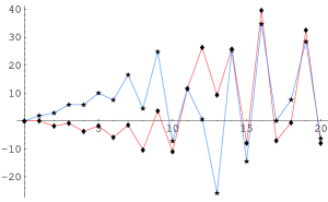
(a) $F_{0}$: both components

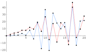
(b) $F_{1}$: both components

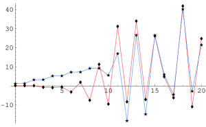
(c) $F_{2}$: both components

Figure 1: Generic behavior of the rank 2 case. Component values are plotted against time step values.

It is a hallmark of the integrability of Painlevé systems that they possess special solutions such as rational and hypergeometric functions [21]. A remarkable discovery of our numerical investigations is that (2.3ad) displays special solution type behavior. These solutions only occur for specific parameter values and initial conditions. One example of this comes at a surprisingly close set of parameters and initial conditions to those displayed by figure 1. By setting the parameters to be

$$B_{0}=\left(\begin{array}[]{ c c }-\infty&0\\ 0&-\infty\end{array}\right)\qquad\,B_{1}=\left(\begin{array}[]{ c c }-\infty&0\\ \frac{3}{5}&-\infty\end{array}\right)$$

with the same set of initial conditions, the behavior coalesces down to the much simpler form shown in figure 2.

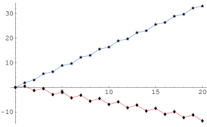
(a) $F_{0}$: both components

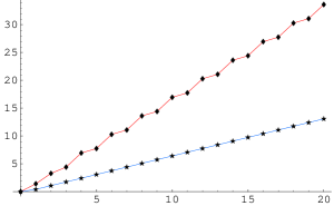
(b) $F_{1}$: both components

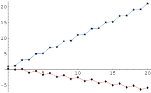
(c) $F_{2}$: both components

Figure 2: Some special behavior of the rank 2 case.

The graphs of the single components in figure 2 strongly resemble the recently discovered ultradiscrete hypergeometric functions of [16]. This implies that the special solution behavior shown here may be parameterized by a higher-dimensional generalization of the ultradiscrete hypergeometric functions of [16]. We discuss this possibility further in section 6. Behavior resembling rational solutions has also been observed in our computational investigations.

The typical behavior of the rank 3 map is shown in figure 3. The initial conditions and parameter values are

$$B_{0}=\left(\begin{array}[]{ c c c }-\infty&\frac{1}{5}&-\infty\\ -\infty&-\infty&\frac{1}{4}\\ -3&-\infty&-\infty\end{array}\right)\,\qquad B_{1}=\left(\begin{array}[]{ c c c }-\infty&-\infty&\frac{1}{7}\\ \frac{3}{5}&-\infty&-\infty\\ -\infty&-\frac{1}{2}&-\infty\end{array}\right)$$

$$F_{0}=\left(\begin{array}[]{ c c c }-2&-\infty&-\infty\\ -\infty&1&-\infty\\ -\infty&-\infty&3\end{array}\right)\,\qquad F_{1}=\left(\begin{array}[]{ c c c }-\frac{1}{4}&-\infty&-\infty\\ -\infty&-5&-\infty\\ -\infty&-\infty&1\end{array}\right)$$

where the coupling comes from the forms of the parameters.

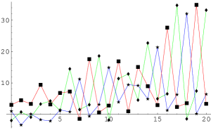
(a) $F_{0}$: all 3 components

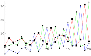
(b) $F_{1}$: all 3 components

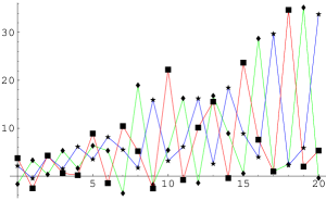
(c) $F_{2}$: all 3 components

Figure 3: Generic behavior of the rank 3 case .

We also find behavior which we conjecture to be parameterized by higher-dimensional ultradiscrete hypergeometric functions. For initial conditions and parameters

$$B_{0}=\left(\begin{array}[]{ c c c }-\infty&0&-\infty\\ -\infty&-\infty&0\\ 0&-\infty&-\infty\end{array}\right)\,\qquad B_{1}=\left(\begin{array}[]{ c c c }-\infty&-\infty&0\\ \frac{3}{5}&-\infty&-\infty\\ -\infty&0&-\infty\end{array}\right)$$

$$F_{0}=\left(\begin{array}[]{ c c c }0&-\infty&-\infty\\ -\infty&0&-\infty\\ -\infty&-\infty&0\end{array}\right)\,\qquad F_{1}=\left(\begin{array}[]{ c c c }0&-\infty&-\infty\\ -\infty&0&-\infty\\ -\infty&-\infty&0\end{array}\right)$$

we obtain the behavior exhibited in figure 4.

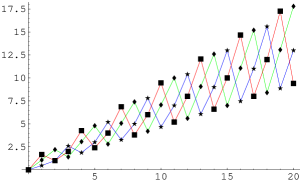
(a) $F_{0}$: all 3 components

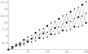
(b) $F_{1}$: all 3 components

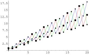
(c) $F_{2}$: all 3 components

Figure 4: Some special behavior of the rank 3 case .

6 Conclusions and discussion

We have presented a noncommutative generalization of $q$-$\mathrm{P}_{\mathrm{IV}}$. Conditions were derived such that the matrix valued systems could be ultradiscretized. In section 4, the matrix generalization of ultradiscrete $\mathrm{P}_{IV}$ was presented. In section 5, a small snapshot of the rich phenomenology was presented. Due to space restrictions, only certain aspects of this phenomenology was presented, yet our preliminary findings suggest many avenues for future research, including the generalization of the results in [16] to higher dimensional ultradiscrete hypergeometric functions.

It is worth noting that a different generalization of $q$-$\mathrm{P}_{\mathrm{IV}}$, has been studied by Kajiwara et al. [12], [13]. It would be interesting to know how both generalizations can be combined.

Appendix A Miscellaneous properties of the group $G$

By deducing properties of the group $G$ presented in (2.3h), we may deduce properties of our elements $\{s_{i}\}$ and $\{z_{i}\}$ since the $\{s_{i}\}$ must be homomorphic images of the generators of $G$, while the $\{z_{i}\}$ are determined by the $\{s_{i}\}$ via (2.3d).

Proposition 1

$$g_{0}^{6}=g_{1}^{6}=g_{2}^{6}.$$ (2.3aa)

Proof Constraint (2.3e) implies

$$g_{2}^{2}=g_{1}^{-2}g_{0}^{4}=g_{1}^{4}g_{0}^{-2}.$$

Therefore $g_{0}^{6}=g_{1}^{6}$, and similarly we have the full proof. $\square$

(Note that this implies $[g_{i},g_{j}^{6}]=0$.)

Proposition 2

Group elements $\{g_{i}\}$ have order 18.

Proof As $g_{1}^{6}=g_{0}^{6}$ it follows from constraints (2.3e) and (2.3f) that

$$g_{0}^{8}=g_{2}^{2}g_{0}^{2}g_{2}^{-2}.$$

Hence

$$g_{0}^{24}=g_{2}^{2}g_{0}^{6}g_{2}^{-2}=g_{0}^{6}$$

and therefore

$$g_{0}^{18}=I.$$ (2.3ab)

The proofs of

$$g_{1}^{18}=I\qquad,\qquad g_{2}^{18}=I$$

proceed in the same manner. $\square$

Proposition 3

$$[g_{i}^{3},g_{j}^{3}]=0.$$ (2.3ac)

Proof Using (2.3aa), equation (2.3g) shows us that

$$g_{0}^{6}=g_{1}^{-3}g_{0}^{-3}g_{1}^{-3}g_{0}^{-3},$$

further application of (2.3aa) reveals

$$g_{0}^{9}=g_{0}^{-6}g_{1}^{3}g_{0}^{-3}g_{1}^{-3},$$

hence, using (2.3ab),

$$g_{0}^{-3}g_{1}^{3}=g_{1}^{3}g_{0}^{-3}.$$

Therefore we have the commutativity of $g_{0}^{3}$ and $g_{1}^{3}$, and similarly we obtain (2.3ac). $\square$

References

References

- [1] Balandin S P and Sokolov V V 1998 On the Painlevé test for non-abelian equations. Phys. Lett. A 246 267–272
- [2] Bobenko A I and Suris Yu B 2002 Integrable non-commutative equations on quad-graphs. The consistency approach. Lett. Math. Phys. 6̱1(3) 241–254
- [3] Bunina E I and Mikhalëv A V 2005 Automorphisms of the semigroup of invertible matrices with nonnegative elements. Fundam. Prikl. Mat. 11 (2) 3–23.
- [4] Field C M, Nijhoff F W and Capel H W 2005 Exact solutions of quantum mappings from the lattice KdV as multi-dimensional operator difference equations. J. Phys. A 38 9503–9527
- [5] Grammaticos B, Ohta Y, Ramani A, Takahashi D and Tamizhmani K M 1997 Cellular automata and ultra-discrete Painlevé equations. Phys. Lett. A 226 53–58
- [6] Grammaticos B and Ramani A 2004 Discrete Painlevé equations: a review. Discrete integrable systems Lecture Notes in Phys. 644 Springer Berlin 245–321
- [7] Isojima S, Grammaticos B, Ramani A and Satsuma J 2006 Ultradiscretization without positivity J. Phys. A 39 3663 -3672
- [8] Joshi N, Nijhoff F W, and Ormerod C 2004 Lax pairs for ultra-discrete Painlevé cellular automata. J. Phys. A 37 L559–L565
- [9] Joshi N and Lafortune S 2005 How to detect integrability in cellular automata J. Phys. A 38 (28) L499–L504
- [10] Joshi N and Ormerod C 2007 The general theory of linear difference equations over the invertible max-plus algebra. Yet to appear
- [11] Kajiwara K, Noumi M, and Yamada Y 2001 A study on the fourth -Painlevé equation. J. Phys. A 34 8563–8581
- [12] Kajiwara K, Noumi M, and Yamada Y 2002 Discrete dynamical systems with symmetry. Lett. Math. Phys. 60 211–219
- [13] Kajiwara K, Noumi M, and Yamada Y 2002 -Painlevé systems arising from -KP hierarchy. Lett. Math. Phys. 62 259–268
- [14] Mikhailov A V and Sokolov V V 2000 Integrable odes on associative algebras. Comm. Math. Phys. 211 231–251
- [15] Olver P J and Sokolov V V 1998 Integrable evolution equations on associative algebras. Comm. Math. Phys. 193 245–268
- [16] Ormerod C 2006 Ultradiscrete hypergeometric solutions to Painlevé equations. Preprint nlin.SI/0610048
- [17] Painlevé P 1900 Mémoire sur les équations différentielles dont l’intégrale générale est uniforme. Bull. Soc. Math. France 28 201–261
- [18] Papageorgiou V G, Nijhoff F W, Grammaticos B and Ramani A 1992 Isomonodromic deformation problems for discrete analogues of Painlevé equations. Phys. Lett. A 164(1) 57–64
- [19] Quispel G R W, Capel H W, and Scully J 2001 Piecewise-linear soliton equations and piecewise-linear integrable maps. J. Phys. A 34 2491–2503
- [20] Ramani A, Grammaticos B and Hietarinta J 1991 Discrete versions of the Painlevé equations. Phys. Rev. Lett. 67 1829–1832
- [21] Ramani A, Grammaticos B, Tamizhmani T, and Tamizhmani K M 2001 Special function solutions of the discrete Painlevé equations. Comp. and Math. with App. 42 603–614
- [22] Ramani A, Takahashi D, Grammaticos B and Ohta Y 1998 The ultimate discretisation of the Painlevé equations Phys. D 114 (3-4) 185–196
- [23] Sakai H 2001 Rational surfaces associated with affine root systems and geometry of the Painlevé equations Comm. Math. Phys. 220 165–229
- [24] Tokihiro T, Takahashi D, Matsukidaira J and Satsuma J 1996 From soliton equations to integrable cellular automata through a limiting procedure. Phys. Rev. Lett. 76 3247–3250