Synchronization of mutually coupled chaotic lasers in the presence of a shutter

Abstract

Two mutually coupled chaotic diode lasers exhibit stable isochronal synchronization in the presence of self feedback. When the mutual communication between the lasers is discontinued by a shutter and the two uncoupled lasers are subject to self-feedback only, the desynchronization time is found to scale as $A_{d}\tau$ where $A_{d}>1$ and $\tau$ corresponds to the optical distance between the lasers. Prior to synchronization, when the two lasers are uncorrelated and the shutter between them is opened, the synchronization time is found to be much shorter, though still proportional to $\tau$. As a consequence of these results, the synchronization is not significantly altered if the shutter is opend/closed faster than the desynchronization time. Experiments in which the coupling between two chaotic-synchronized diode lasers is modulated with an electro-optic shutter are found to be consistent with the results of numerical simulations.

Chaotic systems are characterized by an irregular motion which is sensitive to initial conditions and tiny perturbations. Nevertheless, two chaotic systems can synchronize their irregular motion when they are coupled Pikovsky . When the coupling is switched off, any tiny perturbation drives the two trajectories apart. The separation is exponentially fast, and it is described by the largest Lyapunov exponents of a single system.

In this Letter we show that the trajectory dynamics of coupled chaotic systems which also poses time-delayed self-feedback, is different. In a system with self-feedback, which has also been investigated in the context of secure communication with chaotic lasers MCPF , the time scale for the separation of the trajectories is found to be much longer than the coupling time. On the other hand, when the coupling is switched on, resynchronization occurs on a faster time scale. We investigate this phenomenon numerically and show first experiments which support our numerical simulations. The demonstrated difference between de- and re-synchronization can be used to improve the security of public-channel communication with chaotic lasers MCPF .

Semiconductor (diode) lasers subjected to delayed optical feedback are known to displays chaotic oscillations. Two coupled semiconductor lasers exhibit chaos synchronization. Different coupling setups such as unidirectional or mutual coupling and variations of the strength of the self and coupling feedback result in different synchronization states: the two lasers can synchronize in a leader-laggard or anticipated mode shore99 ; locquet01 , as well as in two different synchronization states; achronal synchronization in which the lasers assume a fluctuating leading role, or isochronal synchronization where there is no time delay between the two lasers’ chaotic signals IsoPaper ; elsasser01 ; MCPF ; exception ; Liu1 .

In this Letter we focus on a symmetric setup, the time delay between the lasers is denoted by $\tau_{c}$ and the time delay of the self-feedback is denoted by $\tau_{d}$. In the event of $\tau_{c}=\tau_{d}=\tau$ and for a wide range of the mutual coupling strength, $\sigma$, and the strength of the self-feedback, $\kappa$, the stationary solution is isochronal synchronization IsoPaper ; MCPF ; Gross2006 . The quantity with which we measure the degree of synchronization between the two lasers is the time-dependent cross correlation, $\rho$, defined as

$$\rho(\Delta t)=\frac{\sum_{i}(I_{A}^{i}-<I_{A}^{i}>)\cdot{(I_{B}^{i+\Delta t}-<I_{B}^{i+\Delta t}>})}{\sqrt[]{\sum_{i}(I_{A}^{i}-<I_{A}^{i}>)^{2}\cdot\sum_{i}(I_{B}^{i+\Delta t}-<I_{B}^{i+\Delta t}>)^{2}}}$$

where $I_{A}$ and $I_{B}$ are the time dependent intensities of lasers A and B and the summation is over times indicated by $i$. Isochronal synchronization is defined by the cross correlation, $\rho$, having a dominant peak at $\Delta t=0$.

We control the mutual coupling between the lasers by a shutter, located at a distance $c\tau/2$ from each one of the lasers, where $c$ is the speed of light. When the shutter is open the two lasers are mutually coupled with strength $\sigma$ and with self-feedback $\kappa$. When the shutter is closed the self-feedback, $\kappa_{e}$, is increased to a value of $\sigma+\kappa$ so that the total feedback in the open/closed states remains a constant. This is required so as to prevent a sudden drop in the overall feedback, which would typically destroy the synchronization immediately alhers98 .

The two quantities of interest in this letter are the desynchronization time, $t_{d}$, and the resynchronization time, $t_{r}$. The desynchronization time is defined as the average required time for the correlation to decay to $C_{d}\rho(0)$ where $C_{d}<1$. The time is measured from the moment the shutter is closed and $\rho(0)$ is the average correlation in the isochronal phase. The resynchronization or recovery time is measured after the shutter has remained closed for a long period and the two chaotic lasers are uncorrelated, and $\kappa_{e}=\kappa+\sigma$. The shutter is then opened and the self-coupling strength is reduced to $\kappa$. The resynchronization time is defined as the average time required, from the shutter opening, for $\rho$ to increase from zero to $C_{r}\rho(0)$, where $C_{r}$ is a constant $\leq 1$.

To numerically simulate the system we use the Lang-Kobayashi equations Kobayashi that are known to describe a chaotic diode laser. The dynamics of laser $A$ are given by coupled differential equations for the optical field, $E$, the time dependent optical phase, $\Phi$, and the excited state population, $n$;

$$\frac{dE_{A}}{dt}=\frac{1}{2}G_{N}n_{A}E_{A}(t)+\frac{C_{sp}\gamma[N_{sol}+n_{A}(t)]}{2E_{A}(t)}~{}~{}~{}~{}~{}~{}~{}~{}~{}~{}~{}~{}~{}~{}~{}~{}~{}~{}~{}~{}~{}~{}~{}~{}~{}~{}~{}$$

$$+\kappa E_{A}(t-\tau_{d})cos[\omega_{0}\tau+\Phi_{A}(t)-\Phi_{A}(t-\tau_{d})]~{}~{}~{}~{}~{}~{}~{}~{}~{}~{}~{}~{}~{}~{}~{}~{}~{}$$

$$+\sigma E_{B}(t-\tau_{c})cos[\omega_{0}\tau_{c}+\Phi_{A}(t)-\Phi_{B}(t-\tau_{c})]~{}~{}~{}~{}~{}~{}~{}~{}~{}~{}~{}~{}~{}~{}$$

$$\frac{d\Phi_{A}}{dt}=\frac{1}{2}\alpha G_{N}n_{A}~{}~{}~{}~{}~{}~{}~{}~{}~{}~{}~{}~{}~{}~{}~{}~{}~{}~{}~{}~{}~{}~{}~{}~{}~{}~{}~{}~{}~{}~{}~{}~{}~{}~{}~{}~{}~{}~{}~{}~{}~{}~{}~{}~{}~{}~{}~{}~{}~{}~{}~{}~{}~{}~{}~{}~{}~{}~{}~{}~{}~{}~{}$$

$$-\kappa\frac{E_{A}(t-\tau_{c})}{E_{A}(t)}sin[\omega_{0}\tau+\Phi_{A}(t)-\Phi_{A}(t-\tau_{d})]~{}~{}~{}~{}~{}~{}~{}~{}~{}~{}~{}~{}~{}~{}~{}~{}~{}$$

$$-\sigma\frac{E_{B}(t-\tau_{c})}{E_{A}(t-\tau_{c})}sin[\omega_{0}\tau_{c}+\Phi_{A}(t)-\Phi_{B}(t-\tau_{c})]~{}~{}~{}~{}~{}~{}~{}~{}~{}~{}~{}~{}~{}~{}~{}$$

$$\frac{dn_{A}}{dt}=(p-1)J_{th}-\gamma n_{A}(t)-[\Gamma+G_{N}n_{A}(t)]E_{A}^{2}(t)~{}~{}~{}~{}~{}~{}~{}~{}~{}~{}~{}~{}~{}~{}~{}~{}~{}~{}~{}$$

and likewise for laser B. The values and meaning of the parameters are those used in Ref. alhers98 ; IsoPaper ; MCPF . The tunable parameters, both in the simulations and in the experiment, are $\kappa$, $\sigma$ and $p$ the pump parameter which is the ratio of the actual laser injection current to the threshold current.

Figure 1 displays the calculated desynchronization time as a function of $\tau$ for $\kappa=\sigma=50ns^{-1}$, $\rho(0)>0.99$, p=1.2, and $C_{d}=0.8$ and $0.9$. Each data point is averaged over $50$ samples, and $\rho(0)$ is measured by averaging a sliding window (sliding length is $1$ ns) over a length $\tau$, while the solid lines are obtained by a linear fit, $t_{d}=A_{d}\tau+constant$. The calculation shows that $t_{d}$ scales linearly with $\tau$ with a slope which increase as $C_{d}$ decreases, and is near $7$ and $9$ for $C_{d}=0.9$ and $0.8$, respectively. A similar linear scaling of the desynchronization time was obtained for all values of $p$ in the range from $1$ to $1.5$, where for a given $C_{d}$, $t_{d}$ decreases with $p$. The simulation assumes an ideal shutter with instantaneous closing and opening times, and also assumes a discontinuous decrease of $\sigma$ to zero while $\kappa$ increases to $\kappa+\sigma$. We find that the linear scaling as well as the slope is robust to the following two experimentally necessitated perturbations: (a) a non-ideal shutter which closes gradually over a period of $10-20$ nanoseconds; (b) an imperfectly closed shutter, allowing residual mutual coupling of a few percent of $\sigma$ while in the closed state.

In the inset of Figure 1, the average $\rho$ as a function of time for $\tau=50$ $ns$ is presented for a case where the shutter was closed at t=0. It is clear that the decay of $\rho$ does not consist of a typical exponential decay. The striking result is that the correlation coefficient is almost a constant for a long initial period (first $\sim 250$ $ns$ for the parameters of figure 1) and then crosses over to an exponential decay for very long times. Because the event of closing or opening the shutter takes a time $\tau/2$ to propagate to the lasers it is reasonable to expect that $t_{d}$ ¿ $\tau/2$. It is surprising, however, that $t_{d}$ scales linearly with $\tau$ with a prefactor which is significantly greater than $1$. It is also not obvious from the simulation (in which $\rho(0)>0.99$),if such behavior can be observed in an experiment where $\rho(0)\leq 0.9$.

The nearly constant value of $\rho$ after the coupling between the lasers is terminated calls for a theoretical explanation. Let us discuss the synchronization for the case $\kappa\sim\sigma$ where both lasers are driven by an almost identical delayed signal which is the sum of the self-feedback and the coupling beam. When the mutual coupling is switched off and replaced with stronger self-feedback, the system still feels its synchronized state for a period of length $\tau$, since the system is coupled to its history delayed by a time $\tau$. The only difference caused by the closing of the shutter is that the lasers no longer communicate with each other and each laser is coupled only to its own state. With time, a small difference in the driving signals develops. This small difference is amplified, since the system is chaotic, and this occurs stepwise in time intervals of length $\tau$. For each interval there is a constant distance between the two trajectories, which increases for the following interval. Only the envelope of these steps is described by the largest Lyapunov exponents, but not the dynamics itself. Hence desynchronization is very slow, and its time scale should be proportional to $\tau$. On the other hand, when the exchanged beam is switched on again, both lasers receive immediately an identical feedback signal (for $\kappa=\sigma$) and synchronize very fast, independent of $\tau$. We thus expect that the desynchronization time is insensitive to the values of $\kappa$ and $\sigma$ and should scale with $\tau$. In contrast the resynchronization time should be very sensitive to the difference, $\kappa-\sigma$.

Figure 1: $t_{d}$ as a function of $\tau$ for p=1.2, $\kappa=\sigma=50ns^{-1}$ and $C_{d}=0.9$ ($\blacksquare$) and $C_{d}=0.8$ ($\bullet$). The lines are a result of a linear fit and the error bars obtained from 50 independent calculations for each point. Inset: The average $\rho$ as a function of time for the same parameters as in the main figure and $\tau=50ns^{-1}$.

The experimental setup, which confirms many of these numerical perdictions, is shown schematically in Figure 2. We use two semiconductor lasers emitting at $660$ $nm$ and operated close to their threshold currents. The temperature of each laser is stabilized to better than $0.01K$. The lasers are subjected to similar optical feedback and are mutually coupled by injecting a fraction of each one’s output power to the other. A fast electro-optic modulator, with measured closing/opening time of 15 $ns$, is introduced in the middle of the coupling optical path to enable closing and reopening of the mutual coupling. The optical setup is designed so as to compensate the sudden drop in the overall feedback power when the shutter is closed and the mutual coupling feedback drops to near zero. We thus use the shutter as a polarization beam splitter which divides the output power of the laser into two parts: one used for the self-feedback and the other for the mutual coupling channels. The opening and closing of the shutter merely changes the ratio of powers in the channels, but maintains the overall feedback power at a constant level. Without this precaution the sudden drop in feedback power would destroy synchronization immediately. This setup, however, does not prevent the change in phase of the laser field when the shutter changes its state. This residual effect decreases the level of synchronization by a small amount (as can be seen in Figure 3). The shutter also does not close hermetically and the leakage power to the mutual coupling channel in the closed state is measured to be $\sim$ 7% of the shutter open value.

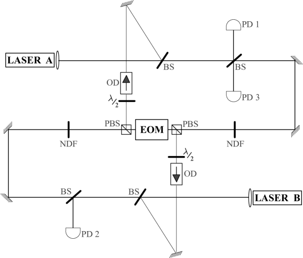
Figure 2: Schematic of the two mutually coupled lasers. EOM - Electro-optic modulator; BS - Beam Splitter; PBS - Polarizing Beam Splitter; OD - Optical Isolator; NDF - Neutral Density Filter; PD - Photodetector.

The feedback strength of each laser is adjusted using a $\lambda/$2 wave plate and an optical diode (see Figure 2) and is set to a value which leads to a reduction of about 5$\%$ in the solitary laser’s threshold current Gross2006 . The lengths of the self-feedback and coupling optical paths are set to be equal to obtain stable isochronal synchronization MCPF . Two sets of measurements are reported here, corresponding to two self-feedback optical paths with $\tau$ = $12.7$ $ns$ and $\tau$ = $23.6$ $ns$.

Two fast photodetectors (response time $<$ 500 $ps$) are used to monitor the laser intensities which are simultaneously recorded with a digital oscilloscope (500 MHz ,1 GS/sec). The correlation coefficient, $\rho$, is calculated by dividing the intensity traces into 10 $ns$ segments (each segment containing 10 points) and $\rho$ is calculated between matching segments and then averaged.

The measured correlation coefficient, $\rho$, is shown in Figure 3, in which the shutter is closed at t=0. The coupling power decays to its closed level in about 15 $ns$, limited by the speed of the shutter. The observed decay time is only slightly shorter than the decay time obtained in simulations for the same $\tau$, and as in the simulations, $\rho$ initially maintains a high and nearly constant value for $50-100$ $ns$, which is much longer than $\tau$. The four data curves shown in the figure correspond to different experimental parameters, indicated by the value of $p$ and to the two different values of $\tau$.

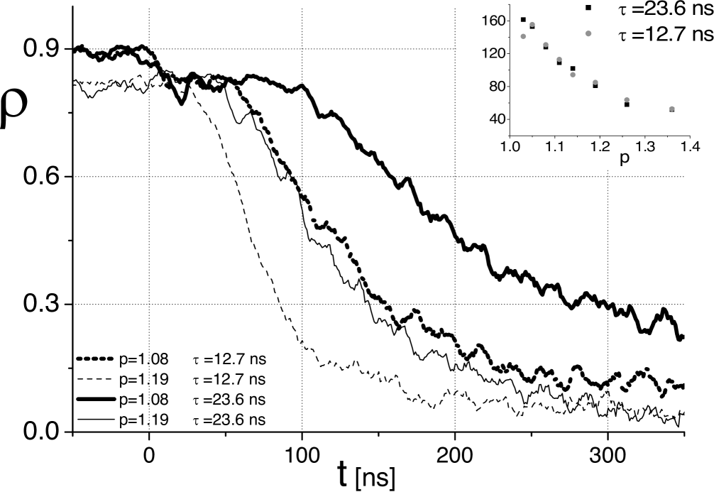
Figure 3: Experimental results for $\rho$ as function of $t$ for $p=1.08,~{}1.19$ and $\tau=12.7,~{}23.6$ $ns$ . Each data point was averaged over 500 measurements. Inset: Data collapse, $1.7\cdot t_{d}$ ($t_{d}$) measured in $ns$ as a function of $p$ for $\tau=12.7$ $ns$ ($23.6$ $ns$).

Figure 3 shows that $t_{d}$ increases with $\tau$ and the inset of Figure 3, depicting $t_{d}$ as a function $p$, indicates that $t_{d}$ is a decreasing function of $p$. The inset of Figure 3 also demonstrates that the different decay curves all collapse to a single decay curve, independent of $p$, when scaled by a factor of $1.7$ which is very close to the ratio of $\tau_{1}/\tau_{2}=23.6/12.7\sim 1.86$. The numerical simulations for larger $\tau$ also exhibit such data collapse when scaled by $\sim\tau_{1}/\tau_{2}$ resulting in scaled decay curves which are independent of $p$prep . This result and the linear scaling of $t_{d}$ for a given $p$ indicate

$$t_{d}(\tau,p)\propto\tau g(p)$$ (1)

where $g(p)$ is a function characteristic of the specific diode laser used. For small $\tau$ finite size effects are expected as a result of the positive constant in the linear scaling shown in Figure 1. Indeed, for $\tau=12.7$ and $23.6$ $ns$, the numerical results indicate that the average ratio $t_{d}(\tau_{1},p)/t_{d}(\tau_{2},p)\sim 1.75$, which is in surprisingly good agreement with the experimental result of $1.7$.

The simulations also indicate that a transition from the low frequency fluctuation (LFF) regime to the fully developed coherent collapse regime FCDC occurs at $p\sim 1.35$, which is close to the experimental value of $p$ (inset of Figure 3) where $t_{d}$ becomes almost independent of $p$prep . Though the decay time obtained from the simulations is longer that the decay time observed in the experiment, this is not surprising, since in the simulations the systems are initially correlated to a very high level ($\rho(0)>0.99$) while in the experiments the initial correlation is $\rho(0)\leq 0.9$

We now turn to examine the scaling of the resynchronization time or the recovery time as a function of $\tau$. In the simulations we start with two uncoupled systems with self-feedback $\kappa_{e}=\kappa+\sigma$. When the shutter is opened at $t=0$, $\kappa_{e}$ is reduced discontinuously to $\kappa$ and the mutual coupling is set to $\sigma$. For all examined cases, with $\kappa\neq\sigma$, our calculations indicate that the resynchronization time also scales linearly with $\tau$. This scaling is exemplified in Figure 4 for $C_{r}=0.9$, $\kappa=60ns^{-1}$ and $\sigma=40ns^{-1}$.

Figure 4: $t_{r}$ as a function of $\tau$ for $p=1.2$, $\kappa=60ns^{-1}$ and $\sigma=40ns^{-1}$. Inset: $t_{r}$ as a function of $\kappa-\sigma$ for $\tau=15$ $ns$.

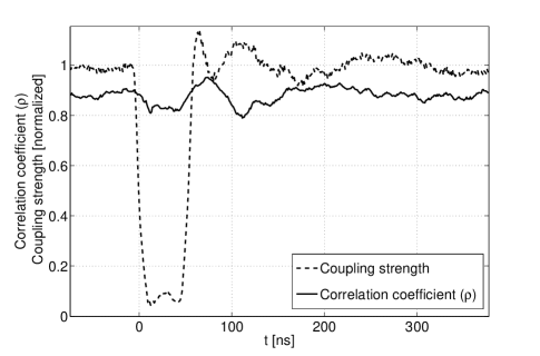
Figure 5: Normalized coupling strength, $\sigma$, (dashed line) and correlation strength, $\rho$, (black line) as a function of time.

The inset of Figure 4 displays the resynchronization time as a function of $\kappa-\sigma$ for a given $\tau$. It appears that this difference, rather than the coupling strength itself, is what controls the resynchronization time, and $t_{r}$ scales almost linearly and symmetrically with $\kappa-\sigma$. For $\kappa=\sigma$, $t_{r}$ is very fast and simulations indicate that it is independent of $\tau$ (limited by the fixed size of the sliding window) as expected. In all examined cases, the prefactor of the linear scaling of the resynchronization time was found to be $\ll A_{d}$, indicating $t_{r}<t_{d}$. We also observed similar behavior, i. e. $t_{r}<t_{d}$, in the experiment, though quantitative determination of the experimental resynchronization time is complicated by ringing in the high voltage electronics used to turn on the modulator and by the fact that the modulator response time is as long as 15 $ns$, which is comparable to $t_{r}$.

Although experimentally we cannot accurately measure the resynchronization time, we show, in Figure 5, a demonstration of the persistence of the synchronization between the lasers upon repeated closing-opening operations of the shutter. Shown is the typical behavior of $\rho$ while the shutter is closed for $\sim 40$ $ns$ and then reopened. The other parameters of the experiment are $\tau=12.6$ $ns$ and $p\sim 1.08$. The cross correlation coefficient $\rho$ is not affected, by the closing/reopening of the shutter and the changing of $\kappa_{e}$ and $\sigma$, since $t_{d}>40$ $ns$.

The results reported above for re/de-synchronization times, which were also obtained recently for chaotic maps prep , demonstrate the possibility of establishing a reliable chaos based communication channel even while the communication between the lasers is interrupted by relatively long intervals. We expect that these effects will play an important role in advanced secure communications using mutually chaotic lasers.

References

- (1) A. Pikovsky, M. Rosenblum and J. Kurths, Synchronization, Cambridge Univ. Press (2003).
- (2) E. Klein, N. Gross, E. Kopelowitz, M. Rosenbluh, L. Khaykovich, W. Kinzel and I. Kanter Phys. Rev. E. (in press) and cond-mat/0604569.
- (3) S. Sivaprakasam and K.A. Shore, Opt. Lett. 24, 466 (1999).
- (4) A. Locquet, F. Rogister, M. Sciamanna, P. Megret, and M. Blondel, Phys. Rev. E 64, 045203(R) (2001).
- (5) E. Klein, N. Gross, M. Rosenbluh, W. Kinzel, L. Khaykovich and I. Kanter. Phys. Rev. E. 73, 066214 (2006).
- (6) T. Heil ,I. Fischer, W. Elsässer, J. Mulet and C. Mirasso, Phys. Rev. Lett. 86, 795 (2001);
- (7) P. Rees, P.S. Spencer, I. Pierce, S. Sivaprakasam, and K.A. Shore, Phys. Rev. A 68, 033818 (2003).
- (8) R. Vicente, S. Tang, J. Mulet, C.R. Mirasso and J.M. Liu, Phys. Rev. E 70, 046216 (2004).
- (9) N. Gross, W. Kinzel, I. Kanter, M. Rosenbluh and L. Khaykovich, Opt. Comm. (in press) and nlin.CD/0604068.
- (10) V. Alhers, U. Parlitz, and W. Lauterborn, Phys. Rev. E 58, 7208 (1998);
- (11) R. Lang, and K. Kobayashi, IEEE J. Quantum Electron. QE-16, 347 (1980).
- (12) T. Heil, I. Fischer, and W. Elsasser, Phys. Rev. A 58, R2672 (1998)
- (13) W. Kinzel et. al. (unpublished).