Statistical Approach of Modulational Instability in the Class of Derivative Nonlinear Schrödinger Equations

Abstract

The modulational instability (MI) in the class of NLS equations is discussed using a statistical approach (SAMI). A kinetic equation for the two-point correlation function is studied in a linear approximation, and an integral stability equation is found. The modulational instability is associated with a positive imaginary part of the frequency. The integral equation is solved for different types of initial distributions ($\delta$- function, Lorentzian) and the results are compared with those obtained using a deterministic approach (DAMI). The differences between MI of the normal NLS equation and derivative NLS equations is emphasized.

Keywords:NLS equations, modulational instability

PACS: 05.45

1. Introduction

The modulational instability (MI - also known as Benjamin-Feir instability) is a well known phenomenon encountered, in quite general conditions, almost each time a quasi-monochromatic wave propagates in a weakly nonlinear medium (Dodd et al 1982, Remoissenet 1999, Scott 2003, Benjamin and Feir 1967, Bespalov et al 1966 and Abdullaev et al 2002). It is responsible for the generation of robust, localized excitations, the solitons in completely integrable systems, and solitary waves in non-integrable ones.

Two different ways to discuss this phenomenon are possible. The first one is a deterministic approach (DAMI) in which the amplitude of a plane wave, with an amplitude dependent dispersion relation (a Stokes wave), is slowly modulated

$$\Psi(x,t)=a\left(1+\varepsilon A(x,t)\right)\exp\left(\mathbf{i}(kx-\omega t)\right)$$ (1)

This approach is well known and can be found in any textbook on nonlinear physics (see Dodd et al 1982, Remoissenet 1999). The second approach is a statistical one (SAMI), and its aim is to see the influence of the statistical properties of the medium on the MI phenomenon. It is a less used approach, but in the last ten years was intensively applied to investigate different physical situations (Alber 1978, Janssen 1983, Fedele et al. 2000, Hall et al 2002, Lisak et al 2002, Fedele et al 2002, Onorato et al 2003), ranging from hydrodynamics (Janssen 1983, Fedele et al. 2000, Hall et al 2002, Lisak et al 2002, Fedele et al 2002), to plasma physics (Fedele 2002), large amplitude wave-envelope propagation in nonlinear media, high-energy accelerators, condensed matter. Recently it was extended also to discrete systems (Visinescu et al 2003, Grecu D. et al 2005) and to systems of coupled nonlinear equations (Manakov’s system) (Grecu D. et al 2004 and 2005).

In this approach a kinetic equation for the two-point correlation function

$$\rho(x_{1},x_{2})=\left<\Psi(x_{1})\,\Psi^{*}(x_{2})\right>$$ (2)

is written down and a linear stability analysis near an initial distribution

$$\rho_{0}(x_{1},x_{2})=\rho_{0}(\left|x_{1}-x_{2}\right|)$$ (3)

is performed. The initial state is assumed homogenous and consequently $\rho_{0}$ depends only on $|x_{1}-x_{2}|$. In the previous expression of $\rho(x_{1},x_{2})$ by $\left<\ldots\right>$ we understand a statistical average over the distribution function of the medium.

The aim of this paper is to investigate MI, especially using the statistical approach of the following equation

$$\mathbf{i}\frac{\partial\Psi}{\partial t}+{1\over 2}\frac{\partial^{2}\Psi}{\partial x^{2}}+\lambda|\Psi|^{2}\Psi+\mathbf{i}\mu|\Psi|^{2}\frac{\partial\Psi}{\partial x}+\mathbf{i}\nu\frac{\partial|\Psi|^{2}}{\partial x}\Psi=0$$ (4)

It is an extended NLS equation, and for different choises of the real parameters $\lambda,\mu,\nu$ several completely integrable equations are recovered. If $\mu=\nu=0$, we get the well known NLS equation

$$\mathbf{i}\frac{\partial\Psi}{\partial t}+{1\over 2}\frac{\partial^{2}\Psi}{\partial x^{2}}+\lambda|\Psi|^{2}\Psi=0$$ (5)

while for $\lambda=0,\mu=\nu$ one obtains the completely integrable derivative NLS-I equation (dNLS I) (Kaup 1978, Nakamura et al. 1980, Mio et al 1976, Mjølhus 1976)

$$\mathbf{i}\frac{\partial\Psi}{\partial t}+{1\over 2}\frac{\partial^{2}\Psi}{\partial x^{2}}+\mathbf{i}\mu\frac{\partial}{\partial x}\left(|\Psi|^{2}\Psi\right)=0$$ (6)

and for $\lambda=\nu=0$ we get another integrable derivative NLS II equation (dNLS II) (Chen, Lee 1979)

$$\mathbf{i}\frac{\partial\Psi}{\partial t}+{1\over 2}\frac{\partial^{2}\Psi}{\partial x^{2}}+\mathbf{i}\mu|\Psi|^{2}\frac{\partial\Psi}{\partial x}=0$$ (7)

Before starting the SAMI study of eq. (4), let us briefly recall the results of a DAMI analysis. Introducing (1) in (4) and keeping only the linear terms in $\varepsilon$ a linear evolution equation for $A(x,t)$ is found. Looking for plane wave solutions of it

$$A(x,t)=\alpha_{1}\mathrm{e}^{\mathbf{i}(Qx-\Omega t)}+\alpha_{2}^{*}\mathrm{e}^{-\mathbf{i}(Qx-\Omega^{*}t)}$$

the compatibility condition of the homogenous system leads us to

$$\Omega-Q\left[k+(\mu+\nu)|a|^{2}\right]=\mathbf{i}Q\sqrt{(\lambda-\nu|a|^{2}-\mu k)|a|^{2}-\frac{Q^{2}}{4}}$$ (8)

an the instability is related to $\mathrm{Im}\Omega>0$. For $\lambda\neq 0$ and denoting $\lambda_{1}=\lambda-\nu|a|^{2}$ we obtain

$$\mathrm{Im}\Omega=Q\sqrt{(\lambda_{1}-\mu k)|a|^{2}-\frac{Q^{2}}{4}}$$ (9)

and one sees that the instability regions depend on the sign of $\mu$. In a $(Q^{2},\,k)$ representation these are given in Fig. 1 (arbitrary units)

Figure 1: Instability regions $(\lambda\neq 0)$; (a) $\mu<0$, (b) $\mu>0$.

It is interesting to consider the instability regions for the two integrable dNLS equations. For dNLS I an instability arises only if $\mu<0$. We have

$$\mathrm{Im}\Omega=Q\sqrt{|\mu||a|^{2}(k-|\mu||a|^{2})-\frac{Q^{2}}{4}}$$ (10)

and in a $(Q^{2},\,k)$ representation the instability occurs only if $k>|\mu||a|^{2}$. For dNLS II the same condition, $\mu<0$, must be fulfilled and

$$\mathrm{Im}\Omega=Q\sqrt{|\mu||a|^{2}k-\frac{Q^{2}}{4}}$$ (11)

The instability regions in $(Q^{2},\,k)$ representation (arbitrary units) are presented in Fig. 2.

Figure 2: Instability regions of the integrable dNLS equations: (a) dNLS I, (b) dNLS II

These results have to be compared with the similar result obtained for NLS equation (5), which writes

$$\mathrm{Im}\Omega=Q\sqrt{\lambda|a|^{2}-\frac{Q^{2}}{4}}$$ (12)

We see that in the NLS case the instability region is independent on the wave vector $k$ of the carrying wave, and restricted to the long wave-length region ($Q^{2}<4\lambda|a|^{2}$), while for all the situations discussed above they are $k$-dependent, and more over they are not restricted to the long wavelength region (exception is the case (b) of Fig 1). Actually for the dNLS equations the long wavelength region is either forbidden, or highly unfavourable for the development of the MI.

In the next section the kinetic equation for the two-point correlation function (2) is obtained and its stability is studied in the linear approximation. An integral stability equation will be obtained and solved for different initial distributions in section 3 ($\delta$-distribution, Lorentzian). Few conclusions and comments are given in the last section. Preliminary results have been presented in Grecu, A.T. 2005.

2. Kinetic equation. Linear stability analysis

The kinetic equation for the two-point correlation function (2), is obtained easily in the following way:

1. write the equation (4) for $x=x_{1}$ and multiply by $\Psi^{*}(x_{2})$;

2. write the complex conjugated of (4) for $x=x_{2}$ and multiply by $\Psi(x_{1})$;

3. add the two equations and take the statistical average;

4. finally use a Gaussian approximation to decouple the four-point correlation functions.

As an illustration we give below two examples of such decouplings

$$\left<\Psi(x_{1})\Psi^{*}(x_{1})\Psi(x_{1})\Psi^{*}(x_{2})\right>=2\overline{a^{2}}(x_{1})\rho(x_{1},x_{2})$$

$$\left<\Psi(x_{1})\Psi^{*}(x_{1})\frac{\partial\Psi(x_{1})}{\partial x_{1}}\Psi^{*}(x_{2})\right>=$$

$$=\overline{a^{2}}(x_{1})\frac{\partial}{\partial x_{1}}\rho(x_{1},x_{2})+\rho(x_{1},x_{2})\lim_{x_{2}\to x_{1}}\frac{\partial}{\partial x_{1}}\rho(x_{1},x_{2})$$

where

$$\overline{a^{2}}(x_{1})=\left<\Psi(x_{1})\Psi^{*}(x_{1})\right>$$ (13)

The kinetic equation found in this way is

$$\mathbf{i}\frac{\partial\rho}{\partial t}+{1\over 2}\left(\frac{\partial^{2}}{\partial x_{1}^{2}}-\frac{\partial}{\partial x_{2}^{2}}\right)\rho+2\lambda\left[\overline{a^{2}}(x_{1})-\overline{a^{2}}(x_{2})\right]\rho$$

$$+\mathbf{i}(\mu+\nu)\left[\overline{a^{2}}(x_{1})\frac{\partial}{\partial x_{1}}+\overline{a^{2}}(x_{2})\frac{\partial}{\partial x_{2}}\right]\rho$$ (14)

$$+\mathbf{i}(\mu+\nu)\rho\left[\lim_{x_{2}\to x_{1}}\frac{\partial}{\partial x_{1}}+\lim_{x_{1}\to x_{2}}\frac{\partial}{\partial x_{2}}\right]\rho$$

$$+2\mathbf{i}\nu\rho\left[\lim_{x_{2}\to x_{1}}\frac{\partial}{\partial x_{1}}+\lim_{x_{1}\to x_{2}}\frac{\partial}{\partial x_{2}}\right]\rho^{*}=0$$

The next step is to introduce the new set of variables

$$x=x_{1}-x_{2}\;\;\;\mathrm{relative\>coordinate}$$ (15)

$$X={1\over 2}(x_{1}+x_{2})\;\;\mathrm{center\>of\>mass\>coordinate}$$

and make a Fourier transform with respect to the relative coordinate. This procedure is known as the Wigner-Moyal transform (Wigner 1932, Moyal 1949) (also known as Klimontovich’s statistical average method, Toda et al 1995), and is very useful to deal with non-homogenous evolution equations. The Fourier transform is defined as

$$F(k,X,t)={1\over{2\pi}}\int_{-\infty}^{+\infty}{\,\mathrm{d}x\,\mathrm{e}^{-\mathbf{i}kx}\rho(x,X,t)}$$ (16)

Using the definition (13) of $\overline{a^{2}}$, it is easily seen that

$$\overline{a^{2}}(X,t)=\int_{-\infty}^{+\infty}{\,\mathrm{d}k\,F(k,X,t)}$$ (17)

After straightforward calculations the Fourier transform of (2.) is given by

$$\frac{\partial F}{\partial t}+k\frac{\partial F}{\partial X}+4\lambda\sum_{j=0}^{\infty}\frac{(-1)^{j}}{(2j+1)\,!\,2^{2j+1}}\frac{\partial^{2j+1}\overline{a^{2}}(X)}{\partial X^{2j+1}}\frac{\partial^{2j+1}F(k,X)}{\partial k^{2j+1}}$$

$$+(\mu+\nu)\frac{\partial\overline{a^{2}}(X)}{\partial X}F(k,X)+2\nu\frac{\partial\left[\overline{a^{2}}(X)\right]^{*}}{\partial X}F(k,X)$$ (18)

$$+(\mu+\nu)\sum_{j=0}^{\infty}{\frac{(-1)^{j}}{2j\,!2^{2j}}\frac{\partial^{2j}\overline{a^{2}}(X)}{\partial X^{2j}}\frac{\partial}{\partial X}\frac{\partial^{2j}F(k,X)}{\partial k^{2j}}}$$

$$-2(\mu+\nu)\sum_{j=0}^{\infty}{\frac{(-1)^{j}}{(2j+1)\,!\,2^{2j+1}}\frac{\partial^{2j+1}\overline{a^{2}}(X)}{\partial X^{2j+1}}\frac{\partial^{2j+1}\left[kF(k,X)\right]}{\partial k^{2j+1}}}=0$$

In obtaining (2.) we have expanded $\overline{a^{2}}(x_{1})=\overline{a^{2}}(X+{x\over 2})$ and $\overline{a^{2}}(x_{2})=\overline{a^{2}}(X-{x\over 2})$ in power series around the point $X$, and we have used the relation

$$x^{j}\,\mathrm{e}^{-\mathbf{i}kx}=(i)^{j}\frac{\partial^{j}}{\partial k^{j}}\mathrm{e}^{-\mathbf{i}kx}$$

Also we used

$$\lim_{x_{2}\to x_{1}}\frac{\partial}{\partial x_{1}}\rho(x_{1},x_{2})=\lim_{x\to 0}\left({1\over 2}\frac{\partial}{\partial X}+\frac{\partial}{\partial x}\right)\int_{-\infty}^{+\infty}{\,\mathrm{d}k\,\mathrm{e}^{\mathbf{i}kx}F(k,X)}=$$

$$={1\over 2}\frac{\partial\overline{a^{2}}(X)}{\partial X}+\mathbf{i}k\overline{a^{2}}(X)$$

and similar expressions for the other limits which appear in (2.).

For a linear stability analysis we consider

$$F(k,X,t)=f(k)+\varepsilon\mathcal{F}(k,X,t)$$ (19)

and

$$\overline{a^{2}}(X,t)=\overline{a^{2}_{0}}+\varepsilon\overline{a^{2}_{1}}(X,t)$$ (20)

where

$$\overline{a^{2}_{0}}=\int_{-\infty}^{+\infty}{\,\mathrm{d}k\,f(k)},~{}~{}~{}~{}~{}\overline{a^{2}_{1}}(X,t)=\int_{-\infty}^{+\infty}{\,\mathrm{d}k\,\mathcal{F}(k,X,t)}$$ (21)

Here $f(k)$ is the Fourier transform of $\rho_{0}(|x|)$, which, due to the homogenous assumption of the initial state, depends only on $k$, and moreover is an even function of $k$.

The linearized kinetic equation in the $(k,X)$ representation is given by

$$\frac{\partial\mathcal{F}}{\partial t}+[k+(\mu+\nu)\overline{a^{2}_{0}}]\frac{\partial\mathcal{F}}{\partial X}+(\mu+\nu)f\frac{\partial\overline{a^{2}_{1}}}{\partial X}+2\nu f\left(\frac{\partial\overline{a^{2}_{1}}}{\partial X}\right)^{*}$$

$$+4\lambda\sum_{j=0}^{\infty}\frac{(-1)^{j}}{(2j+1)\,!\,2^{2j+1}}\frac{\partial^{2j+1}\overline{a^{2}_{1}}(X)}{\partial X^{2j+1}}\frac{\partial^{2j+1}f(k)}{\partial k^{2j+1}}$$ (22)

$$-2(\mu+\nu)\sum_{j=0}^{\infty}\frac{(-1)^{j}}{(2j+1)\,!\,2^{2j+1}}\frac{\partial^{2j+1}\overline{a^{2}_{1}}(X)}{\partial X^{2j+1}}\frac{\partial^{2j+1}(kf(k))}{\partial k^{2j+1}}=0$$

The last step is to look for a plane wave solution of (2.)

$$\mathcal{F}(k,X,t)=g_{1}(k)\mathrm{e}^{\mathbf{i}(QX-\Omega t)}+g_{2}^{*}(k)\mathrm{e}^{-\mathbf{i}(QX-\Omega^{*}t)}$$ (23)

$$\overline{a^{2}_{1}}(X,t)=G_{1}\mathrm{e}^{\mathbf{i}(QX-\Omega t)}+G_{2}^{*}\mathrm{e}^{-\mathbf{i}(QX-\Omega^{*}t)}$$

where

$$G_{i}=\int_{-\infty}^{+\infty}{g_{i}(k)}\,\mathrm{d}k\,,\;\;i=1,2$$ (24)

Introducing (23) into (2.) the following equation is found

$$(k-\omega)g_{1}+(\mu+\nu)fG_{1}+2\nu fG_{2}$$

$$+{{2\lambda}\over Q}\left[f(k+{Q\over 2})-f(k-{Q\over 2})\right]G_{1}$$ (25)

$$-\frac{\mu+\nu}{Q}\left[h(k+{Q\over 2})-h(k-{Q\over 2})\right]G_{1}=0$$

Here we denoted $\omega={\Omega\over Q}-(\mu+\nu)\overline{a^{2}_{0}}$ and $h(k)=kf(k)$. Also we used

$$2\sum_{j=0}^{\infty}\frac{1}{(2j+1)\,!}\left({Q\over 2}\right)^{2j+1}\frac{\partial^{2j+1}f(k)}{\partial k^{2j+1}}=f(k+{Q\over 2})-f(k-{Q\over 2})$$

and a similar relation for $h(k)$.

In (2.) we have to divide by $(k-\omega)$ and integrate over $k$. Introducing the notations

$$I=\int_{-\infty}^{+\infty}{\frac{f(k)}{k-\omega}\,\mathrm{d}k\,}$$

$$J=\int_{-\infty}^{+\infty}{\frac{f(k+{Q\over 2})-f(k-{Q\over 2})}{k-\omega}\,\mathrm{d}k\,}$$ (26)

$$K=\int_{-\infty}^{+\infty}{\frac{h(k+{Q\over 2})-h(k-{Q\over 2})}{k-\omega}\,\mathrm{d}k\,}$$

the following homogenous algebric linear equation in $G_{1}$ and $G_{2}$ is obtained

$$G_{1}+(\mu+\nu)IG_{1}+2\nu IG_{2}+{{2\lambda}\over Q}JG_{1}-\frac{\mu+\nu}{Q}KG_{1}=0$$ (27)

A second equation is found starting from the complex conjugated of (2.), namely

$$G_{2}+(\mu+\nu)IG_{2}+2\nu IG_{1}+\frac{2\lambda}{Q}JG_{2}-\frac{\mu+\nu}{Q}KG_{2}=0$$ (28)

The compatibility condition for the system (27),(28) leads us to the following integral stability equations

$$1+(\mu-\nu)I+\frac{2\lambda}{Q}J-\frac{\mu+\nu}{Q}K=0$$

or

$$1+(\mu+3\nu)I+\frac{2\lambda}{Q}J-\frac{\mu+\nu}{Q}K=0$$

In the next section these will be solved for different initial conditions $f(k)$.

3. Solution of the integral stability equation

The first distribution function we shall discuss is a $\delta$-spectrum

$$f(k)=\overline{a^{2}_{0}}\delta(k)$$ (29)

It doesn’t describe a realistic situation as it coresponds to a constant two-point correlation function in the initial state, $\rho_{0}=\overline{a^{2}_{0}}=const.$. But the calculations are easily done and can be considered as a limit case to which more realistic situations can be compared. The integrals $I,J,K$ are immediatly calculated

$$I=-\frac{\overline{a^{2}_{0}}}{\omega},\;J=\frac{\overline{a^{2}_{0}}Q}{\omega^{2}-{{Q^{2}}\over 4}},\;K=0$$ (30)

Then both integral equations (A) and (B) become an algebraic equation of third order in $\omega$

$$\omega^{3}-\bar{\mu}\overline{a^{2}_{0}}\omega^{2}+(2\lambda\overline{a^{2}_{0}}-{{Q^{2}}\over 4})\omega+\bar{\mu}\overline{a^{2}_{0}}{{Q^{2}}\over 4}=0$$ (31)

where $\bar{\mu}=\mu_{A}=\mu-\nu$ for A-equation and $\bar{\mu}=\mu_{B}=\mu+3\nu$ for B-equation. With $\omega=y+{1\over 3}\bar{\mu}\overline{a^{2}_{0}}$ it is reduced to the canonical form

$$y^{3}+py+q=0$$ (32)

where

$$p=2\lambda\overline{a^{2}_{0}}-{1\over 3}(\bar{\mu}\overline{a^{2}_{0}})^{2}-{{Q^{2}}\over 4}$$

$$q={2\over 3}\bar{\mu}\overline{a^{2}_{0}}\left[\lambda\overline{a^{2}_{0}}-{1\over 9}(\bar{\mu}\overline{a^{2}_{0}})^{2}+{{Q^{2}}\over 4}\right]$$ (33)

Complex solutions of (32) are obtained if the discriminant $\Delta=\left({p\over 3}\right)^{3}+\left({q\over 2}\right)^{2}$ is positive. The sign of $\Delta$ is controlled by the sign of $p$. For $\lambda\neq 0$ we have $p>0$ if $Q^{2}/4<2\lambda\overline{a^{2}_{0}}-{1\over 3}(\bar{\mu}\overline{a^{2}_{0}})^{2}$, corresponding to the long wavelength region. With the notations

$$\sqrt{\frac{p^{3}}{27}}={q\over 2}\tan\alpha,\;\;\tan\varphi=\sqrt[3]{\tan{\alpha\over 2}}$$ (34)

we have

$$\mathrm{Im}\,\omega=\frac{\sqrt{p}}{\sin 2\varphi}$$ (35)

But if $p<0$ we can still have $\Delta>0$. Writing

$${{Q^{2}}\over 4}=2\lambda\overline{a^{2}_{0}}-{1\over 3}(\bar{\mu}\overline{a^{2}_{0}})^{2}+3\tilde{Q}^{2}$$ (36)

the condition $\Delta>0$ leads us to the inequality

$$\tilde{Q}^{3}-\bar{\mu}\overline{a^{2}_{0}}\tilde{Q}^{2}<\bar{\mu}\overline{a^{2}_{0}}\left[\lambda\overline{a^{2}_{0}}-{4\over 27}(\bar{\mu}\overline{a^{2}_{0}})^{2}\right]$$ (37)

In this case ($\Delta>0$ and $p<0$) the usual notations are

$$\sqrt{-\frac{p^{3}}{27}}={q\over 2}\sin\alpha,\;\;\tan\varphi=\sqrt[3]{\tan{\alpha\over 2}}$$

and one obtaines

$$\mathrm{Im}\,\omega=\sqrt{-p}\cot 2\varphi$$

The instability remains in the long wavelength region.

When $\lambda=0$ the situation is completely changed. Then

$$p=-\left[{{Q^{2}}\over 4}+{1\over 3}(\bar{\mu}\overline{a^{2}_{0}})^{2}\right]$$

$$q={2\over 3}\mu\overline{a^{2}_{0}}\left[{{Q^{2}}\over 4}-{1\over 9}(\bar{\mu}\overline{a^{2}_{0}})^{2}\right]$$ (38)

and $\Delta>0$ can be realized only if $Q>{2\over 3}\bar{\mu}\overline{a^{2}_{0}}$. This means that the instability develops for higher wave vectors $Q$, a result in complete agreement to the conclusions of the DAMI analysis of the derivative NLS equations. Using the same notations ($34^{\prime}$) we get the same result ($35^{\prime}$), and the requirement $\Delta>0$ reduces to

$$\left({q\over 2}\right)^{2}>-\left({p\over 3}\right)^{3}$$ (39)

an inequality from which the limit value of ${{Q^{2}}\over 4}$ can be calculated.

A more realistic situation is a Lorentzian distribution

$$f(k)={\overline{a^{2}_{0}}\over\pi}\frac{\sigma}{k^{2}+\sigma^{2}}$$ (40)

which corresponds to an exponential decaying two-point correlation function in the initial state

$$\rho_{0}(x)=\overline{a^{2}_{0}}\mathrm{e}^{-\sigma x}\;x>0$$ (41)

The integrals I, J, K are easily calculated in the $k$-complex plane assuming $\omega$ complex with $\mathrm{Im}\,\omega>0$. We obtain

$$I=-\frac{\overline{a^{2}_{0}}}{\tilde{\omega}}$$

$$J=\frac{\overline{a^{2}_{0}}Q}{\tilde{\omega}^{2}-{Q^{2}\over 4}}$$ (42)

$$K=\frac{-\mathbf{i}\sigma\overline{a^{2}_{0}}Q}{\tilde{\omega}^{2}-{Q^{2}\over 4}}$$

where $\tilde{\omega}=\omega+\mathbf{i}\sigma$, and the instability condition $\mathrm{Im}\,\omega>0$ becomes for the new variable $\tilde{\omega}$, $\mathrm{Im}\,\tilde{\omega}>\sigma$.

To have a point of reference, let us recall the result for the usual NLS equation ($\mu=\nu=0$) (Visinescu et al 2003, Grecu D. et al (2004, 2005), Grecu A.T. 2005)

$$\mathrm{Im}\,\omega=\sqrt{2\lambda\overline{a^{2}_{0}}-{Q^{2}\over 4}}-\sigma$$ (43)

We get $\mathrm{Im}\,\omega>0$ if

$$Q<2\sqrt{2\lambda\overline{a^{2}_{0}}-\sigma^{2}}$$ (44)

which shows that the MI is restricted to the long wave-length region and is strongly dependent on the correlation length in the initial state; if $\sigma^{2}>2\lambda\overline{a^{2}_{0}}$, the initial state is stable to small modulations.

When (42) are introduced in (A) and (B), we get again an algebraic equation of third order in $\tilde{\omega}$, but now with complex coefficients. It can be reduced to the canonical form with

$$p=2\left(\lambda+{\mathbf{i}\over 2}\overline{\nu}\sigma\right)\overline{a^{2}_{0}}-{1\over 3}(\overline{\mu}\overline{a^{2}_{0}})^{2}-{Q^{2}\over 4}$$ (45)

$$q={2\over 3}\overline{\mu}\overline{a^{2}_{0}}\left[\left(\lambda+{\mathbf{i}\over 2}\overline{\nu}\sigma\right)\overline{a^{2}_{0}}-{1\over 9}(\overline{\mu}\overline{a^{2}_{0}})^{2}+{Q^{2}\over 4}\right]$$

where $\overline{\mu}$ has the same meaning as in the case of the $\delta$-spectrum, and $\overline{\nu}=\mu+\nu$. As mentioned before the MI region coresponds to $\mathrm{Im}\,\tilde{\omega}>\sigma$.

Instead of working on the general case let us consider only the situations of the dNLS equations. We shall start with the dNLS-II equation ($\lambda=\nu=0$). Then both equations (A) and (B) reduce to a single equation

$$1-\mu\overline{a^{2}_{0}}{1\over\tilde{\omega}}+\mathbf{i}\mu\overline{a^{2}_{0}}\frac{\sigma}{\tilde{\omega^{2}}-{Q^{2}\over 4}}=0$$ (46)

It is convenient to measure $\tilde{\omega},\,\sigma\,\mathrm{and}\,Q$ in units of $|\mu|\overline{a^{2}_{0}}$. If $\varepsilon=\mathrm{sgn}\,\mu$, the following algebraic equation of third order is found:

$$\tilde{\omega}^{3}-\varepsilon\tilde{\omega}^{2}-\left({Q^{2}\over 4}-\mathbf{i}\varepsilon\sigma\right)\tilde{\omega}+\varepsilon{Q^{2}\over 4}=0$$ (47)

It has a certain symmetry having solutions of the form $\tilde{\omega}=\varepsilon\tilde{\omega}_{r}+\mathbf{i}\tilde{\omega}_{i}$. As we are interested in the imaginary part of these solutions, the result is independent on the sign of $\mu$. The equation (47) is solved numerically. Measuring $\Omega$ in units of $(\mu\overline{a^{2}_{0}})^{2}$, one has $\mathrm{Im}\,\Omega=Q(\mathrm{Im}\,\tilde{\omega}-\sigma)$. A three dimensional plot , $\mathrm{Im}\,\Omega$ function of $\sigma$ and $Q^{2}/4$ is given in Fig. 3 As one sees, the neighbourhood of $Q=0$ is excluded from the instability region, which extends on a finite domain of $Q$ and $\sigma$. One can find a limit value for $\sigma\,(\sigma_{C}\simeq 0.194)$ and the MI exists only for $\sigma<\sigma_{C}$.

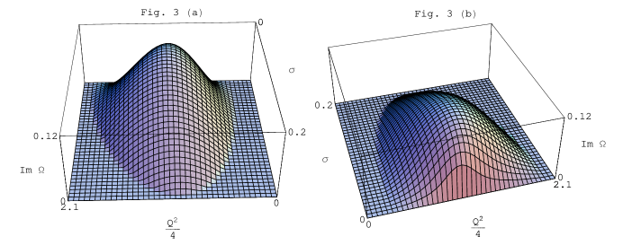
Figure 3: Instability region for dNLS I. Three dimensional plot of $\mathrm{Im}\,\Omega$ versus $Q^{2}/4$ and $\sigma$; Two different orientantions.

Now let us consider the case of dNLS-I equation ($\lambda=0,\,\mu=\nu$). The equation (A) becomes

$$1+2\mathbf{i}\frac{\mu\overline{a^{2}_{0}}}{\tilde{\omega}^{2}-{Q^{2}\over 4}}=0$$ (48)

which is easily solved giving

$$\mathrm{Im}\,\tilde{\omega}={1\over\sqrt{2}}\left[\sqrt{\left({Q^{2}\over 4}\right)^{2}+4(\mu\overline{a^{2}_{0}})^{2}}-{Q^{2}\over 4}\right]^{1/2}$$ (49)

and the MI region is determined by

$$Q^{2}<4\left[\left(\frac{\mu\overline{a^{2}_{0}}}{\sigma}\right)^{2}-\sigma^{2}\right],\;\sigma^{2}<\mu\overline{a^{2}_{0}}$$ (50)

This instability region is located near the origin in the plane $(Q,\,\sigma)$.

Another instability region results from (B), which writes

$$\tilde{\omega}^{3}-4\varepsilon\tilde{\omega}^{2}-\left({Q^{2}\over 4}-2\mathbf{i}\varepsilon\sigma\right)\tilde{\omega}+4\varepsilon{Q^{2}\over 4}=0$$ (51)

where as in the case of dNLS-II, we measure $\tilde{\omega},\,\sigma$ and $Q$ in units of $|\mu|\overline{a^{2}_{0}}$. This equation has the same form as (46). The instability region is obtained numerically and is represented in Fig. 4. Again the $Q\simeq 0$ region is excluded and one finds a critical value $\sigma_{c}\simeq 0.441$ for $\sigma$, which determines the superior limit of the MI region.

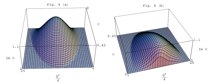
Figure 4: Instability region for dNLS II. Three dimensional plot of $\mathrm{Im}\,\Omega$ versus $Q^{2}/4$ and $\sigma$; Two different orientantions.

4. Conclusions

Several conclusions result from this analysis. For the extended NLS equation (4) the instability region in a DAMI analysis is dependent on the wave-vector $\vec{k}$ of the carrying wave. In the case of derivative NLS equations the long wave-length region is either forbidden, or highly unfavourable for the development of MI.

In the SAMI instead of the $k$-dependence the instability region is now dependent on the correlation length in the initial 2-point correlation function. Although we got explicit results only for a $\delta-$ and Lorentzian distribution function we conclude that the MI is possible only for long-range correlations in the initial state. In the case of a $\delta$-function initial distribution, in a limit situation corresponding to an infinite correlation length, the results are similar with those obtained from DAMI analysis; for the dNLS equations again the long wave-length region is highly unfavourable. The same conclusions can be drawn for the more realistic case of a Lorentzian initial distribution function, namely that the MI region is restricted to a finite region of ($Q,\;\sigma$) plane containing the axis $\sigma=0$. A critical value $\sigma_{c}$ is determined for both dNLS equations and again the $Q\simeq 0$ region is unfavourable for the instability development.
Another realistic initial condition is a Gaussian distribution function

$$f(k)=\overline{a^{2}}{0}{1\over\sqrt{2\pi}\sigma}\mathrm{e}^{-\frac{k^{2}}{2\sigma^{2}}}$$

Calculations done only for NLS eq. (see Alber 1978) reveal the same conclusions, namely the MI is possible only for long-range correlations in the initial state ($\sigma$ small) and in the long wave-length region. The result is more complicated, being expressed through some special functions (complex integral function $\omega(z)$, Abramowitz and Stegun 1965).

Such calculations for dNLS equations are not yet performed.

The influence of the statistical properties of the medium on the development of large amplitude waves, is a problem of special interest in hydrodynamics, especially for the generation of freak waves in the ocean. In a linear theory there is no interaction between ocean waves. A focusing phenomenon of wave energy may occur only when constructing interference takes place. The situation is competely different when nonlinear wave-wave interaction is present. Then a wave can borrow energy from its neighbours and due to this extra-focusing phenomenon, waves with very high amplitude can be generated. In this process the knowledge of the initial conditions of the oceanic waves is essential. Accordingly, many experimental works have been conducted. For a long time the Joint North Sea Wave Project (JONSWAP) has studied the power spectrum of the oceanic waves (Komen et al 1994), resulting a non-Gaussian expression. It was used to calculate the probability to generate large amplitude oceanic waves (analytically and numerically) in given realistic conditions (Janssen 1983, Onorato et al 2001, 2003, 2004).

Calculations using other initial distribution functions, reflecting different physical situations, would be of real interest for sure, even in the case of derivative NLS equations.

Acknowledgements

The present work was done under the contract CEX-D11-9 with the Ministry of Education and Research from Romania.

5. References

Abdulaev, F.Kh., Darmanyan, S.A., Garnier, J. (2002) in Progress in Optics 44, 303 (ed. E. Wolf, Elsevier)
Abramowitz, M., Stegun, I., (1965) Handbook of Mathematical Functions (National Bureau of Stand)
Alber, I.E. (1978) Proc. Roy. Soc. London A 363, 525
Benjamin, T.B., Feir, J.E., (1967) J. Fluid Mech. 27, 417
Bespalov, V. I., Talanov, V.I., (1966) Prisma JETP 3, 417
Chen, H.H., Lee, Y.C., (1979) Physica Scripta 20, 490
Dodd, R.K., Eilbeck, J.C., Gibbon, J.D., Morris, H.C., (1982) Solitons and Nonlinear Wave Equations (Acad. Press, New York)
Fedele, R., Anderson, D., (2000) J. Opt. B: Quantum Semiclassical Optics 2, 207
Fedele, R., Anderson, D., Lisak, M., (2000) Physica Scripta T 84, 27
Fedele, R., Shukla, P.K., Onorato, M., Anderson, D., Lisak, M., (2002) Phys. Rev. Lett. A 303, 61
Grecu, A.T., Grecu, D., Visinescu, A., (2005) Rom. J. Phys. 50, 127
Grecu, A.T., (2005) Ann. Univ. Craiova, Physics AUC 15 (part I), 177
Grecu, D., Visinescu, A., (2004) in Nonlinear Waves. Classical and Quantum Aspects, p. 151 (eds. F. Kh. Abdulaev, V. V. Konotop, Kluwer Acad. Publ.)
Grecu, D., Visinescu, A., (2005) Theor. Math. Phys. 144, 927
Grecu, D., Visinescu, A., (2005) Rom. J. Phys. 50, 137
Hall, B., Lisak, M., Anderson, D., Fedele, R., Semenov, V.E., (2002) Phys. Rev. E 65, 035602 R
Janssen, P.A.E.M., (1983) J. Fluid Mech. 133, 113
Kaup, D.J., Newell, A.C., (1978) J. Math. Phys. 19, 798
Komen, J.C., Cavaleri, L., Donelan, M., Hasselman, K., Hasselman, S., Jansen, P.A.E.M., (1994) Dynamics and Modelling of Ocean Waves (Cambridge Univ. Press)
Lisak, M., Hall, B., Anderson, D.. Fedele, R., Semenov, V.E., Shukla, P.K., Hasegawa, A., (2002) Physics Scripta T 98, 12
Mio, K., Ogino, T., Minami, K., Takeda, S., (1976) J. Phys. Soc. Japan 41, 265, 667
Mjølhus, E., (1976) J. Plasma Physics 16, 321
Moyal, J.E., (1949) Proc. Cambridge Phyl. Soc. 45, 99
Nakamura, A., Chen, H.H., (1980) J. Phys. Soc. Japan 49, 813
Onorato, M., Osborne, A.R., Serio, M., Bertone, S., (2001) Phys. Rev. Lett. 86, 5831
Onorato, M., Osborne, A., Fedele, R., Serio, M., (2003) Phys. Rev. E 67, 046305
Onorato, M., Osborne, A.R., Serio, M., Cavaleri, L., Brandini, C., Stansberg C.T., (2004) Phys. Rev. E 70, 067302
Remoissenet, M., (1999) Waves Called Solitons (Springer Verlag, Berlin)
Scott, A., (2003) Nonlinear Science. Emergence and Dynamics of Coherent Structures (Oxford Univ. Press)
Visinescu, A., Grecu, D., (2003) Eur. Phys. J. B 34, 225
Visinescu, A., Grecu, D., (2003) Rom. J. Phys. 48, 787
Toda, M., Kubo, R., Saito, N., (1995) Statistical Physics vol. 1 (Springer, Berlin)
Wigner, E., (1932) Phys. Rev. 40, 749