Dynamo effect in the Kraichnan magnetohydrodynamic turbulence

Abstract

The existence of a dynamo effect in a simplified magnetohydrodynamic model of turbulence is considered when the magnetic Prandtl number approaches zero or infinity. The magnetic field is interacting with an incompressible Kraichnan-Kasantzev model velocity field augmented with a viscous scale cutoff. An approximate system of equations in the different scaling ranges can be formulated and solved, so that the solution tends to the exact one when the viscous and magnetic-diffusive cutoffs approach zero. In this approximation we are able to determine analytically the conditions for the existence of a dynamo effect and give an estimate of the dynamo growth rate. Among other things we show that in the large Prandtl number case the dynamo effect is always present. Our analytical estimates are in good agreement with previous numerical studies of the Kraichnan-Kasantzev dynamo by Vincenzi [14].

1 Introduction

As we are lacking in the complete understanding of turbulence, it is useful to study simplified models which share many features of the full problem. One class of models are the passive advection models, where the velocity field is given some predetermined statistics. One then studies the effect of this velocity field on some other quantities such as the passive scalar, a temperature or a dye density in the fluid (see e.g. [4]). The term passive refers to the absence of backreaction to the velocity field. Naturally one would like to extend this study to passively advected vector fields. There exist physically realistic models such as the small resistivity magnetohydrodynamic equations for the magnetic field $\mathbf{B}\in\mathbb{R}^{d}$ interacting with a fluid (see e.g. [6, 14, 13, 1] and references therein)

$$\partial_{t}\mathbf{B}+\mathbf{v}\cdot\nabla\mathbf{B}-\mathbf{B}\cdot\nabla\mathbf{v}=\kappa\Delta\mathbf{B}.$$ (1.1)

We will derive an equation for the pair correlation function

$$\big{\langle}B_{i}(t,\mathbf{r})B_{j}(t,\mathbf{r}^{\prime})\big{\rangle}$$ (1.2)

averaged over the velocity statistics, and attempt to solve it using a certain approximation scheme, which will be explained at the end of this introduction. The $\mathbf{v}$ above is the velocity field of a conducting fluid. It is assumed to be incompressible as in the constant density Navier-Stokes equation, that is, $\nabla\cdot\mathbf{v}=0$. Naturally the magnetic field is also incompressible due to the absence of magnetic charges. $\kappa$ is the resistivity divided by the vacuum permeability. The “smallness” of $\kappa$ here means that the equation is a good approximation when the magnetic Reynolds number $R_{M}=VL/\kappa$ is very large. Here $L$ is the integral scale of the velocity field and $V$ is the r.m.s velocity at such a scale. Since we assume from the beginning that $L\to\infty$, the approximation holds. In reality we should also consider the backreaction of $\mathbf{B}$ on $\mathbf{v}$, but we will only consider the passive case and just assume $\mathbf{v}$ to be given by the Kraichnan statistics (see e.g. [4] for a definition). It is defined as a Gaussian, mean zero velocity field with pair correlation function

$$\big{\langle}v_{i}(t,\mathbf{r})v_{j}(t^{\prime},\mathbf{r}^{\prime})\big{\rangle}=\delta(t-t^{\prime})D_{0}\!\int\!\!d\mathbf{k}\frac{e^{i\mathbf{k}\cdot(\mathbf{r}-\mathbf{r}^{\prime})}}{|\mathbf{k}|^{d+\xi}}f(l_{\nu}|\mathbf{k}|)P_{ij}(\mathbf{k})=:\delta(t-t^{\prime})D_{ij}(\mathbf{r}-\mathbf{r}^{\prime};l_{\nu})$$ (1.3)

with $d\mathbf{k}:=\frac{d^{d}k}{(2\pi)^{3}}$ and

$$P_{ij}(\mathbf{k})=\delta_{ij}-\frac{k_{i}k_{j}}{k^{2}}$$ (1.4)

to guarantee incompressibility. It is evident that $D_{ij}$ is homogenous and isotropic. The parameter $\xi$ for $0\leq\xi\leq 2$ describes the roughness of the velocity field with $\xi=2/3$ corresponding to the Kolmogorov scaling. The function $f$ is an ultraviolet cutoff, which simulates the effects of viscosity. It decays faster than exponentially at large $k$, while $f(0)=1$ and $f^{\prime}(0)=0$. For example we could choose $f(l_{\nu}k)=\exp{(-l_{\nu}^{2}k^{2})}$, although the explicit form of the function is not needed below. In the usual case without the cutoff function $f$ the velocity correlation function behaves as a constant plus a term $\propto r^{\xi}$, but in this case we have an additional scaling range for $r\ll l_{\nu}$ where it scales as $\propto r^{2}$. The length scale $l_{\nu}$ can be used to define a viscosity $\nu$ or alternatively one can use $\kappa$ to define a length scale $l_{\kappa}$. We can then define the Prandtl number measuring the relative effects of viscosity and diffusivity as $P=\nu/\kappa$. Note that the integral scale was assumed to be infinite, i.e. there is no IR cutoff.

In addition to an advection term $\mathbf{v}\cdot\nabla\mathbf{B}$ in Eq. (1.1), familiar from the passive scalar problem, there is also a stretching term $\mathbf{B}\cdot\nabla\mathbf{v}$. This, and the fact that the magnetic field is a vector, will give rise to some interesting deviations from the passive scalar case. The most interesting one is probably the dynamo effect, an unbounded growth of the magnetic field depending on the roughness of the velocity field described by the parameter $\xi$, and the Prandtl number. This is in complete contrast to the passive scalar case, where in the absence of external forcing the dynamics is always dissipative [8].

The dynamo effect has been previously studied by e.g. Kazantsev [9], where he derived a Schrödinger equation for the pair correlation function. However, the equation was still quite difficult to analyze except in some special cases. Some analytical and numerical results have been obtained e.g. in [13] and [14] (see the latter for further references). The goal of the present paper is to extend these considerations by introducing a set of approximate equations, which admit an exact solution. The analysis proceeds along the same lines as in a previous paper for a different problem by one of us [5]. The problem in the analysis can be traced to existence of length scales dividing the equation in different scaling ranges. In our case there are two such length scales, one arising from the diffusivity $\kappa$ and the other from the UV cutoff in the velocity correlation function. As will be seen in appendix A, what one actually needs in the analysis is the velocity structure function defined as

$$\frac{1}{2}\big{\langle} (v_{i}(t,\mathbf{r})-v_{i}(t,\mathbf{r}^{\prime}))(v_{j}(t^{\prime},\mathbf{r})-v_{j}(t^{\prime},\mathbf{r}^{\prime}))\big{\rangle}$$

$$=\delta(t-t^{\prime})D_{0}\!\int\!\!\bar{d}\mathbf{k}\frac{1-e^{i\mathbf{k}\cdot(\mathbf{r}-\mathbf{r}^{\prime})}}{|\mathbf{k}|^{d+\xi}}f(l_{\nu}|\mathbf{k}|)P_{ij}(\mathbf{k})$$

$$=:\delta(t-t^{\prime})d_{ij}(\mathbf{r}-\mathbf{r}^{\prime};l_{\nu})$$ (1.5)

This is all one needs to derive a partial differential equation for the pair correlation function of $\mathbf{B}$, but it will still be very difficult to analyze. Hence the approximation, which proceeds as follows:

1) Consider the asymptotic cases where $r$ is far from the length scales $l_{\kappa}$ and $l_{\nu}$ with the separation of the length scales large as well. There are therefore three ranges where the equation is simplified into a much more manageable form. The equations are of the form $\partial_{t}H-\mathcal{M}H=0$, where $\mathcal{M}$ is a second order differential operator with respect to the radial variable. We then consider the eigenvalue problem $\mathcal{M}h=\lambda h$.

2) By a suitable choice of constant parameters in terms of the length scales, we can adjust the differential equations to match in different regions as closely as possible. Solving the equations, we obtain two independent solutions in all ranges.

3) We match the solutions by requiring continuity and differentiability at the scales $l_{\nu}$ and $l_{\kappa}$. Also appropriate boundary conditions are applied.

4) According to standard physical lore, the form of cutoffs do not affect the results when the cutoffs are removed. In addition to $l_{\nu}$, we can interpret $l_{\kappa}$ as a cutoff. Therefore we conjecture that the solution approaches the exact one for small cutoffs. We also expect the qualitative results, such as the existence of the dynamo effect, to apply for finite cutoffs as well.

For concreteness, suppose that $\mathcal{M}$ is of the form

$$\mathcal{M}=a(l_{\nu},l_{\kappa},r)\partial_{r}^{2}+b(l_{\nu},l_{\kappa},r)\partial_{r}+c(l_{\nu},l_{\kappa},r).$$ (1.6)

The coefficients are some functions of the length scales $l_{\nu}$ and $l_{\kappa}$ and the radial variable $r$. In general, solving the eigenvalue problem for such a differential equation is not possible except numerically. However, we can approximate the coefficients in the asymptotic regions when $r$ is far from the length scales. The asymptotic coefficients are all power laws and solving the equations becomes much easier. Figure 1 illustrates this procedure corresponding to steps $1)$ and $2)$ for any of the coefficients.

After some preparations, we begin by writing down the equation for the pair correlation function of the magnetic field using the Itô formula. The derivation can be found in appendix A. The equation is of third order in the radial variable, but it can be manipulated into a second order equation by using the incompressibility condition. In section 2 the approximate equations will be derived when $\nu\ll\kappa$ and $\kappa\ll\nu$, or Prandtl number small or large, respectively. We use adimensional variables for sake of convenience and clarity. The focus of the paper is mainly on the existence of the dynamo effect and its growth rate. Therefore we consider the spectrum of $\mathcal{M}$. By a spectral mapping theorem, we relate the spectra of $\mathcal{M}$ and the corresponding semigroup $e^{t\mathcal{M}}$. It is then evident that if the spectrum of $\mathcal{M}$ contains a positive part, there is exponential growth, i.e. a dynamo effect.

\psfrag{a}{a)}\psfrag{b}{b)}\psfrag{c}{c)}\psfrag{d}{d)}\psfrag{r}{r}\includegraphics[width=371.0254pt]{matching}

Figure 1: A sketch of the procedure of approximating the example equation. The dashed vertical lines correspond to either one of the length scales $l_{\nu}$ and $l_{\kappa}$ with pictures a) a plot of the “real” coefficient, which depends of the cutoff function (and is really unknown), b) an approximate form obtained by taking $r$ far from the length scales (dotted parts of the lines are dropped) c) the approximations extended to cover all $r\in\mathbb{R}$ and d) adjusting the coefficients to match at the scales $l_{\nu}$ and $l_{\kappa}$. For $r$ much larger than the cutoffs, the error due to the approximation is lost.

1.1 Structure function asymptotics

Due to the viscous scale $l_{\nu}$ in the structure function Eq. (1.5), there are two extreme scaling ranges $r\gg l_{\nu}$ (inertial range) and $r\ll l_{\nu}$. For $r\gg l_{\nu}$ we can set $l_{\nu}=0$ in Eq. (1.5) and obtain

$$d_{ij}^{>}(\mathbf{r}):=D_{1}r^{\xi}\left((d+\xi-1)\delta_{ij}-\xi\frac{r_{i}r_{j}}{r^{2}}\right),$$ (1.7)

where

$$D_{1}=\frac{D_{0}C_{\infty}}{(d-1)(d+2)},\ \ \ \ \ C_{\infty}=\frac{\Gamma(1-\xi/2)}{2^{d+\xi-2}\pi^{d/2}\Gamma(d/2+\xi/2)}.$$ (1.8)

The second case corresponds to the viscous range, which is to leading order in $r$:

$$d_{ij}^{<}(\mathbf{r}):=D_{2}l_{\nu}^{\xi-2}r^{2}\left((d+1)\delta_{ij}-2\frac{r_{i}r_{j}}{r^{2}}\right),$$ (1.9)

where

$$D_{2}=\frac{D_{0}C_{0}}{(d-1)(d+2)},\ \ \ \ \ C_{0}=\!\int\!\!\bar{d}\mathbf{k}\frac{f(k)}{k^{d+\xi-2}}.$$ (1.10)

We see that the viscous range form (1.9) can be obtained from (1.7) by a replacement $\xi\to 2$ and $D_{1}\to D_{2}l_{\nu}^{\xi-2}$. Note that by adjusting the cutoff function $f$ we can also adjust $D_{2}/D_{1}$.

1.2 Incompressibility condition

Due to rotation and translation invariance, the equal-time correlation function of $\mathbf{B}$ must be of the form

$$G_{ij}(t,|\mathbf{x}-\mathbf{x}^{\prime}|):=\langle B_{i}(t,\mathbf{x})B_{j}(t,\mathbf{x}^{\prime})\rangle=G_{1}(t,r)\delta_{ij}+G_{2}(t,r)\frac{r_{i}r_{j}}{r^{2}},$$ (1.11)

where $r=|\mathbf{x}-\mathbf{x}^{\prime}|$. Additional simplification arises from the incompressibility condition $\partial_{i}G_{ij}=0$:

$$\partial_{r}G_{1}=-\frac{1}{r^{d-1}}\partial_{r}(r^{d-1}G_{2}).$$ (1.12)

The general solution of the incompressibility condition can be written as

$$\left\{\begin{array}[]{ll}G_{1}&=rH^{\prime}(r)+(d-1)H(r)\\ G_{2}&=-rH^{\prime}(r)\end{array}\right.$$ (1.15)

In terms of a so far arbitrary function $H$. Alternatively, adding the above equations we may write

$$H(r)=\frac{1}{d-1}\left(G_{1}+G_{2}\right).$$ (1.16)

This observation leads to a considerable simplification in the differential equation for the correlation function: whereas the equations for $G_{1}$ and $G_{2}$ are of third order in $r$, we can use the above result to obtain a second order equation for $H$. Then we would get back to $G$ through Eqs. (1.15); for example we have for the trace of $G$:

$$G_{ii}=(d-1)\left(rH^{\prime}(r)+dH(r)\right),$$ (1.17)

although we refrain from doing this since $H$ has the same spectral properties as $G_{ii}$.

2 Equations of motion

The equation of motion for the pair correlation function is derived in appendix A:

$$\frac{d}{dt}G_{ij}(t,\mathbf{r})=2\kappa\Delta G_{ij}(t,\mathbf{r})+d_{\alpha\beta}G_{ij,\alpha\beta}-d_{\alpha j,\beta}G_{i\beta,\alpha}-d_{i\beta,\alpha}G_{\alpha j,\beta}+d_{ij,\alpha\beta}G_{\alpha\beta}.$$ (2.1)

The indices after commas are used to denote partial derivatives and we use the Einstein summation. By taking $r\gg l_{\nu}$ and $r\ll l_{\nu}$ we can use the approximations (1.7) and (1.9) to write the equation in the corresponding ranges. This is done for the quantity $H=(G_{1}+G_{2})/(d-1)$ in the Appendix A as well, resulting in the equations

$$\frac{dH}{dt} =\xi(d-1)(d+\xi)D_{1}r^{\xi-2}H+\left[2(d+1)\kappa+(d^{2}-1+2\xi)D_{1}r^{\xi}\right]\frac{1}{r}H^{\prime}$$

$$+\left[2\kappa+(d-1)D_{1}r^{\xi}\right]H^{\prime\prime},\ \ \ r\gg l_{\nu}.$$ (2.2)

and

$$\frac{dH}{dt} =2(d-1)(d+2)D_{2}l_{\nu}^{\xi-2}H+\left[2(d+1)\kappa+(d^{2}+3)D_{2}l_{\nu}^{\xi-2}r^{2}\right]\frac{1}{r}H^{\prime}$$

$$+\left[2\kappa+(d-1)D_{2}l_{\nu}^{\xi-2}r^{2}\right]H^{\prime\prime},\ \ \ r\ll l_{\nu}.$$ (2.3)

Simple dimensional analysis leads to the observation

$$[\kappa]=[D_{1}r^{\xi}]=[D_{2}l_{\nu}^{\xi-2}r^{2}],$$ (2.4)

where the brackets denote the scaling dimension of the quantities. We define the length scale $l_{\kappa}$ as the scale below which the diffusive effects of $\kappa$ become important. This will be done explicitly below for different Prandtl number cases. In general, one can write $\kappa=D_{1}l_{\nu}^{\xi-p}l_{\kappa}^{p}$ for some $p\in(0,2]$. Now one just needs to identify the dominant terms in the three scales divided by $l_{\nu}$ and $l_{\kappa}$. For sake of clarity, we choose to write these equations in adimensional variables. This can be done for example by defining $r=l\rho$ and $t=l^{2-\xi}\tau/D_{1}$ with $l$ being a length scale. It turns out to be convenient to choose the larger of $l_{\kappa}$ and $l_{\nu}$ as $l$. Since we deal with a stochastic velocity field with no intrinsic dynamics, we cannot, in principle, talk about viscosity. However, it is convenient to define a viscosity $\nu$ (of dimension length squared divided by time) by dimensional analysis from the length scale $l_{\nu}$ and the dimensional velocity magnitude $D_{1}$, giving a relationship between $\nu$, $l_{\nu}$ and $D_{1}$ similar to what we would get in a dynamical model. We therefore define

$$\nu:=D_{1}l_{\nu}^{\xi}.$$ (2.5)

This permits us to define the Prandtl number in the standard manner as $P=\nu/\kappa$. We then consider the cases $P\ll 1$ and $P\gg 1$.

2.1 Small Prandtl number

\psfrag{a}{$l_{\nu}$}\psfrag{b}{$l_{\kappa}$}\psfrag{c}{$l_{\nu}/l_{\kappa}$}\psfrag{d}{1}\psfrag{r}{$r$}\psfrag{o}{$\rho$}\psfrag{S}{S}\psfrag{M}{M}\psfrag{L}{L}\includegraphics[width=231.89pt]{prline}

Figure 2: Sketch of the scaling ranges at small Prandtl number.

Now $\nu\ll\kappa$, and we choose as adimensional variables

$$\left\{\begin{array}[]{ll}r&=l_{\kappa}\rho\\ t&=\frac{l_{\kappa}^{2-\xi}}{D_{1}}\tau.\end{array}\right.$$ (2.8)

Note that the relation between $l_{\kappa}$ and $\kappa$ has not yet been determined. In these variables the equations (2.2) and (2.3) become

$$\partial_{\tau}H =\xi(d-1)(d+\xi)\rho^{-2+\xi}H+\left[2(d+1)\frac{\kappa}{D_{1}l_{\kappa}^{\xi}}+(d^{2}-1+2\xi)\rho^{\xi}\right]\frac{1}{\rho}\partial_{\rho}H$$

$$+\left[2\frac{\kappa}{D_{1}l_{\kappa}^{\xi}}+(d-1)\rho^{\xi}\right]\partial_{\rho}^{2}H,\ \ \rho\gg l_{\nu}/l_{\kappa}$$ (2.9)

and

$$\partial_{\tau}H =2(d-1)(d+2)\frac{D_{2}}{D_{1}}\left(\frac{l_{\nu}}{l_{\kappa}}\right)^{\xi-2}H+\left[2(d+1)\frac{\kappa}{D_{1}l_{\kappa}^{\xi}}+(d^{2}+3)\frac{D_{2}}{D_{1}}\left(\frac{l_{\nu}}{l_{\kappa}}\right)^{\xi-2}\rho^{2}\right]\frac{1}{\rho}\partial_{\rho}H$$

$$+\left[2\frac{\kappa}{D_{1}l_{\kappa}^{\xi}}+(d-1)\frac{D_{2}}{D_{1}}\left(\frac{l_{\nu}}{l_{\kappa}}\right)^{\xi-2}\rho^{2}\right]\partial_{\rho}^{2}H,\ \ \rho\ll l_{\nu}/l_{\kappa}.$$ (2.10)

As mentioned above, we also consider $r\ll l_{\kappa}$ and $r\gg l_{\kappa}$, that is $\rho\ll 1$ and $\rho\gg 1$, respectively. There are now three regions in $\rho$, divided by $l_{\nu}/l_{\kappa}$ and $1$, with $l_{\nu}/l_{\kappa}\ll 1$. The regions, solutions and various other quantities will be labelled by $S$, $M$ and $L$, corresponding to $\rho\ll l_{\nu}/l_{\kappa}$, $l_{\nu}/l_{\kappa}\ll\rho\ll 1$ and $1\ll\rho$. See Fig. 2 for quick reference. Therefore the short range equation will be derived from Eq. (2.10) and the two others from (2.9). Consider for example explicitly the coefficients of $\partial_{\rho}^{2}H$:

$$L:\ \ \ 2\frac{\kappa}{D_{1}l_{\kappa}^{\xi}}+(d-1)\rho^{\xi}$$

$$M:\ \ \ 2\frac{\kappa}{D_{1}l_{\kappa}^{\xi}}+(d-1)\rho^{\xi}$$ (2.11)

$$S:\ \ \ 2\frac{\kappa}{D_{1}l_{\kappa}^{\xi}}+(d-1)\frac{D_{2}}{D_{1}}\left(\frac{l_{\nu}}{l_{\kappa}}\right)^{\xi-2}\rho^{2}.$$

By definition of the length scale $l_{\kappa}$, in the region $L$ the diffusivity is negligible and in the region $M$ it is dominant, as it is in the region $S$ since in there $\rho$ approaches zero. The coefficients are then approximately

$$L:\ \ \ (d-1)\rho^{\xi}$$

$$M:\ \ \ 2\frac{\kappa}{D_{1}l_{\kappa}^{\xi}}$$ (2.12)

$$S:\ \ \ 2\frac{\kappa}{D_{1}l_{\kappa}^{\xi}}.$$

Matching the coefficients of $L$, $M$ at $\rho=1$ provides us with a condition (matching between $S$ and $M$ gives nothing new)

$$d-1=2\frac{\kappa}{D_{1}l_{\kappa}^{\xi}}.$$ (2.13)

This is used as a definition of $\kappa$ as $\kappa=\frac{1}{2}(d-1)D_{1}l_{\kappa}^{\xi}$. Writing down the short range equation with the above approximations,

$$\partial_{\tau}H_{S}=2(d-1)(d+2)\frac{D_{2}}{D_{1}}\left(\frac{l_{\nu}}{l_{\kappa}}\right)^{\xi-2}H_{S}+(d^{2}-1)\frac{1}{\rho}\partial_{\rho}H_{S}+(d-1)\partial_{\rho}^{2}H_{S},$$ (2.14)

by using the derived expression for the Prandtl number,

$$P=\frac{\nu}{\kappa}=\frac{2}{d-1}\left(\frac{l_{\nu}}{l_{\kappa}}\right)^{\xi},$$ (2.15)

and by defining

$$\frac{D_{2}}{D_{1}}=\left(\frac{2}{d-1}\right)^{1-2/\xi}$$ (2.16)

(remember that $D_{2}$ could be adjusted by a choice of the cutoff function $f$, see Eq. (1.9) and below) a more neat expression is obtained for the short range equation. We can now write down all the equations:

$$\partial_{\tau}H_{S} =\ 2(d-1)(d+2)P^{1-2/\xi}H_{S}+(d^{2}-1)\frac{1}{\rho}\partial_{\rho}H_{S}+(d-1)\partial_{\rho}^{2}H_{S}$$ (2.17a)

$$\partial_{\tau}H_{M} =\ \xi(d-1)(d+\xi)\rho^{-2+\xi}H_{M}+(d^{2}-1)\frac{1}{\rho}\partial_{\rho}H_{M}+(d-1)\partial_{\rho}^{2}H_{M}$$ (2.17b)

$$\partial_{\tau}H_{L} =\ \xi(d-1)(d+\xi)\rho^{-2+\xi}H_{L}+(d^{2}-1+2\xi)\rho^{\xi-1}\partial_{\rho}H_{L}+(d-1)\rho^{\xi}\partial_{\rho}^{2}H_{L}$$ . (2.17c)

2.2 Large Prandtl number

\psfrag{a}{$l_{\kappa}$}\psfrag{b}{$l_{\nu}$}\psfrag{c}{$l_{\kappa}/l_{\nu}$}\psfrag{d}{1}\psfrag{r}{$r$}\psfrag{o}{$\rho$}\psfrag{S}{S}\psfrag{M}{M}\psfrag{L}{L}\includegraphics[width=231.89pt]{prline}

Figure 3: Sketch of the scaling ranges at large Prandtl number.

Now $\nu\gg\kappa$, and we choose

$$\left\{\begin{array}[]{ll}r&=l_{\nu}\rho\\ t&=\frac{l_{\nu}^{2-\xi}}{D_{1}}\tau.\end{array}\right.$$ (2.20)

Then the equations (2.2) and (2.3) for $r\gg l_{\nu}$ and $r\ll l_{\nu}$ become in the new variables

$$\partial_{\tau}H =\xi(d-1)(d+\xi)\rho^{-2+\xi}H+\left[2(d+1)\frac{\kappa}{D_{1}l_{\nu}^{\xi}}+(d^{2}-1+2\xi)\rho^{\xi}\right]\frac{1}{\rho}\partial_{\rho}H$$

$$+\left[2\frac{\kappa}{D_{1}l_{\nu}^{\xi}}+(d-1)\rho^{\xi}\right]\partial_{\rho}^{2}H,\ \ \rho\gg 1$$ (2.21)

and

$$\partial_{\tau}H =2(d-1)(d+2)\frac{D_{2}}{D_{1}}H+\left[2(d+1)\frac{\kappa}{D_{1}l_{\nu}^{\xi}}+(d^{2}+3)\frac{D_{2}}{D_{1}}\rho^{2}\right]\frac{1}{\rho}\partial_{\rho}H$$

$$+\left[2\frac{\kappa}{D_{1}l_{\nu}^{\xi}}+(d-1)\frac{D_{2}}{D_{1}}\rho^{2}\right]\partial_{\rho}^{2}H,\ \ \rho\ll 1.$$ (2.22)

The ranges $S$, $M$ and $L$ now correspond to $\rho\ll l_{\kappa}/l_{\nu}$, $l_{\kappa}/l_{\nu}\ll\rho\ll 1$ and $1\ll\rho$, see Fig. 3. Note that equations in both $S$ and $M$ are now derived from Eq. (2.22). As before, we consider again the coefficients of $\partial_{\rho}^{2}H$ and drop the terms $\propto\kappa$ in $L$ and $\propto\rho^{2}$ in $S$. The diffusive effects are not dominant in the region $M$ since $r\gg l_{\kappa}$, so we drop the $\propto\kappa$ term in $M$ too. The approximative coefficients are then

$$L:\ \ \ (d-1)\rho^{\xi}$$

$$M:\ \ \ (d-1)\frac{D_{2}}{D_{1}}\rho^{2}$$ (2.23)

$$S:\ \ \ 2\frac{\kappa}{D_{1}l_{\nu}^{\xi}}.$$ (2.24)

We then obtain two equations by matching the coefficient of $L$ with $M$ at $\rho=1$ and of $M$ with $S$ at $l_{\kappa}/l_{\nu}$:

$$\frac{D_{2}}{D_{1}}(d-1) =(d-1),$$

$$(d-1)\frac{D_{2}}{D_{1}}\left(\frac{l_{\kappa}}{l_{\nu}}\right)^{2} =2\frac{\kappa}{D_{1}l_{\nu}^{\xi}}$$ (2.25)

with solutions

$$D_{2} =D_{1}$$

$$\kappa =\frac{d-1}{2}D_{1}l_{\kappa}^{2}l_{\nu}^{\xi-2}.$$ (2.26)

The Prandtl number is in this case

$$P=\frac{2}{d-1}\left(\frac{l_{\nu}}{l_{\kappa}}\right)^{2}.$$ (2.27)

Note that one can obtain this from the small Prandtl number equation (2.15) by replacing $\xi\to 2$. This is a reflection of a more subtle observation that the large Prandtl number case for any $\xi$ is similar to the small Prandtl number case with $\xi=2$. We collect the equations using the above approximations,

$$\partial_{\tau}H_{S} =\ 2(d-1)(d+2)H_{S}+2\frac{d+1}{P}\frac{1}{\rho}\partial_{\rho}H_{S}+\frac{2}{P}\partial_{\rho}^{2}H_{S}$$ (2.28a)

$$\partial_{\tau}H_{M} =\ 2(d-1)(d+2)H_{M}+(d^{2}+3)\rho\partial_{\rho}H_{M}+(d-1)\rho^{2}\partial_{\rho}^{2}H_{M}$$ (2.28b)

$$\partial_{\tau}H_{L} =\ \xi(d-1)(d+\xi)\rho^{-2+\xi}H_{L}+(d^{2}-1+2\xi)\rho^{\xi-1}\partial_{\rho}H_{L}+(d-1)\rho^{\xi}\partial_{\rho}^{2}H_{L}$$ . (2.28c)

Note that the short and long range equations are somewhat similar to the respective small Prandtl number ones, Eqs. (2.17a,2.17b,2.17c). However, the equation in the medium range above is scale invariant in $\rho$, unlike the corresponding small Prandtl number one.

3 Resolvent

Given a differential operator $\mathcal{M}$ with a domain $D(\mathcal{M})$, we define the resolvent

$$R(z,\mathcal{M}):=(z-\mathcal{M})^{-1}$$ (3.1)

and the resolvent set as

$$\rho(\mathcal{M}):=\left\{z\in\mathbb{C}|z-\mathcal{M}:D(\mathcal{M})\to\textnormal{X is bijective}\right\}.$$ (3.2)

The complement of the resolvent set, denoted by $\sigma(\mathcal{M})$, is the spectrum of $\mathcal{M}$. According to the Hille-Yosida theorems (see e.g. [2]), if $(\mathcal{M},D(\mathcal{M}))$ is closed and densely defined and if there exists $z_{0}\in\mathbb{R}$ such that for each $z\in\mathbb{C}$ with $\Re{z}>z_{0}$ we have $z\in\rho(\mathcal{M})$, and

$$\parallel R(z,\mathcal{M})\parallel\leq\frac{1}{\Re{z}-z_{0}},$$ (3.3)

then $\mathcal{M}$ is the generator of a strongly continuous semigroup $T(t)$ satisfying

$$\parallel T(t)\parallel\leq e^{z_{0}t}$$ (3.4)

and vice versa. If in addition $\mathcal{M}$ is a so called sectorial operator, meaning that its spectrum is contained in some angular sector $\{z\in\mathbb{C}:|\arg(z-z_{0})|>\alpha>\pi/2\}$ and that outside this sector the resolvent satisfies the (stronger) estimate

$$\parallel R(z,\mathcal{M})\parallel\leq\frac{C}{|z-z_{0}|},$$ (3.5)

then $\mathcal{M}$ generates an analytical semigroup, for which the spectral mapping theorem

$$\sigma\left(T(t)\right)=\{0\}\cup e^{t\sigma(\mathcal{M})}.$$ (3.6)

holds, relating the spectrum of the generator to that of the semigroup. One can also use the Cauchy integral formula

$$T(t):=e^{t\mathcal{M}}=\frac{1}{2\pi i}\int\limits_{\mathcal{C}}dze^{zt}R(z,\mathcal{M}),$$ (3.7)

where the contour surrounds the spectrum $\sigma(\mathcal{M})$.

We do not prove here that $\mathcal{M}$ is sectorial, however we refer the interested reader to the general mathematical theory in [11] where it is explained and substantiated that strongly elliptic operators are, under quite general assumption, sectorial generators, on a wide range of Banach spaces (e.g. $L^{p}$ and $C^{1}$ spaces to name but a few).

According to the above discussion, in order to explain the existence of the dynamo effect and its growth rate, we only need to find the spectrum of $\mathcal{M}$ via the resolvent set $\rho(\mathcal{M})$. Note that we are interested only in the positive part of the spectrum, since we want to determine the existence of the dynamo effect only.

The operator $\mathcal{M}$ in our case is cut up as the operators $\mathcal{M}_{L}$, $\mathcal{M}_{M}$ and $\mathcal{M}_{S}$ in the corresponding ranges, obtained from the equations (2.17a, 2.17b, 2.17c) and (2.28a, 2.28b, 2.28c). The resolvent is found from the equation

$$\left(z-\mathcal{M}\right)R(z,\mathcal{M})(\rho,\rho^{\prime})=\delta(\rho,\rho^{\prime}).$$ (3.8)

Since we are primarily interested in the long range ($L$) behavior $\rho>1$, we let $\rho^{\prime}$ stay in the region $L$ at all times. This results in three equations

$$\left\{\begin{array}[]{ll}\left(z-\mathcal{M}_{L}\right)R_{L}(\rho,\rho^{\prime})&=\delta(\rho-\rho^{\prime})\\ \left(z-\mathcal{M}_{M}\right)R_{M}(\rho,\rho^{\prime})&=0\\ \left(z-\mathcal{M}_{S}\right)R_{S}(\rho,\rho^{\prime})&=0\end{array}\right.$$ (3.12)

where $R_{L}(\rho,\rho^{\prime})$ is the expression of the resolvent for $\rho\in L$ (the large scale range) and $\rho^{\prime}\in\mathbb{R}_{+}$ and similarly $R_{M}$ and $R_{S}$ are valid when $\rho$ is in the middle and small scale ranges respectively. We require the following boundary conditions from the resolvents: for small $\rho$ we are in the diffusion dominated range, so we require smooth behavior at $\rho\to 0$. For large $\rho$ we eventually cross the integral scale (although we haven’t defined it explicitly) above which the velocity field behaves like the $\xi=0$ Kraichnan model, leading to diffusive behavior at the largest scales for which the appropriate condition on the resolvent is exponential decay at infinity.

3.1 Solutions

Assuming $\rho\neq\rho^{\prime}$, we solve the equations (3.12) with the corrsponding operators $\mathcal{M}$.

The operator ${\mathcal{M}}_{L}$ does not depend on the Prandtl number. So in the region $L$, we get from e.g. Eq. (2.28c) (we use lowercase letters $h^{\pm}$ to denote the independent solutions)

$$h_{L}^{\pm}(\rho)=\rho^{-d/2-\frac{\xi}{d-1}}\tilde{Z}_{\lambda}^{\pm}\left(w\rho^{1-\xi/2}\right),$$ (3.13)

where $\tilde{Z}_{\lambda}^{+}\equiv I_{\lambda}$ and $\tilde{Z}_{\lambda}^{-}\equiv K_{\lambda}$ are modified Bessel functions of the first and second kind respectively, and we have introduced

$$w=\frac{2}{2-\xi}\sqrt{\frac{z}{(d-1)}}.$$ (3.14)

and the order parameter $\lambda$ is

$$\lambda=\frac{\sqrt{d[2(d-1)^{3}-(d-2)(2\xi+d-1)^{2}]}}{(2-\xi)(d-1)}.$$ (3.15)

Because the range $S$ is always in the diffusive region, we require smoothness of the solution at zero. Only one of the solutions satisfies this, so we get from Eqs. (2.17a) and (2.28a)

$$h_{S,1}(\rho)=\rho^{-d/2}\ I_{d/2}\left(\sqrt{\frac{z}{d-1}-2(d+2)P^{1-2/\xi}}\rho\right)$$ (3.16)

and

$$h_{S,2}(\rho)=\rho^{-d/2}\ I_{d/2}\left(\sqrt{\frac{z}{2}-(d-1)(d+2)}\sqrt{P}\ \rho\right),$$ (3.17)

where the subindex $1$ refers to $P\ll 1$ (small Prandtl number) and $2$ to $P\gg 1$. We will use this notation in other objects as well.

In the range M, when $P\gg 1$ we have the scale invariant equation in (2.28b) with power law solutions

$$h_{M,2}^{\pm}(\rho)=\rho^{-d/2-\frac{2}{d-1}\pm\zeta},$$ (3.18)

where

$$\zeta=\sqrt{\frac{z-z_{2}}{d-1}}$$ (3.19)

with

$$z_{2}=-\frac{d-1}{4}[(2-\xi)\lambda]^{2}|_{\xi=2}=-\frac{d}{4(d-1)}(d^{3}-10d^{2}+9d+16)\,.$$ (3.20)

The medium range equation for $P\ll 1$ cannot be solved exactly, but we can consider it in two different asymptotic cases. From Eq. (2.17b) we get

$$\left(\xi(d+\xi)\rho^{-2+\xi}-\frac{z}{d-1}\right)R_{M}+(d+1)\frac{1}{\rho}\partial_{\rho}R_{M}+\partial_{\rho}^{2}R_{M}=0$$ (3.21)

and note that since by definition of the medium range $l_{\nu}/l_{\kappa}\ll\rho\ll 1$, i.e. $1<\rho^{-2+\xi}<(l_{\kappa}/l_{\nu})^{2-\xi}$ (the $\ll$ was replaced by $<$, so that things remain valid even as $\xi\to 2$), the term $\propto\rho^{-2+\xi}$ can be dropped if we assume that

$$|z|>(l_{\kappa}/l_{\nu})^{2-\xi}\approx P^{-\frac{2-\xi}{\xi}}\,.$$ (3.22)

If on the other hand we have

$$|z|<1\,,$$ (3.23)

then $z$ can be neglected in the equation.

The solution for large $z$ is similar to the short range solutions,

$$h_{M,1}^{\pm}(\rho)=\rho^{-d/2}\tilde{Z}^{\pm}_{d/2}\left(\sqrt{\frac{z}{d-1}}\rho\right),\ \ \ \ |z|>(l_{\kappa}/l_{\nu})^{2-\xi},$$ (3.24)

where we denoted the $P\ll 1$ case by a subscript $1$. For small $z$ we have instead

$$h_{M,1}^{\pm}=\rho^{-d/2}Z^{\pm}_{d/\xi}\left(2\sqrt{d/\xi+1}\rho^{\xi/2}\right),\ \ \ \ |z|<1.$$ (3.25)

where $Z_{d/\xi}^{+}\equiv J_{d/\xi}$ and $Z_{d/\xi}^{-}\equiv Y_{d/\xi}$ are Bessel functions of the first and second kind respectively. It turns out however that the explicit form of the above solutions affects only a specific numerical multiplier and has no effect on the presence of the dynamo. Because of this we in fact derive a lower bound for the growth rate which in view of the present approximation provides a more reliable result.

3.2 Matching of solutions

Consider equations (3.12). We denote the long range regions $\rho<\rho^{\prime}$ and $\rho>\rho^{\prime}$ as $L_{<}$ and $L_{>}$. The boundary conditions for the resolvent demanded finiteness at $\rho=0$, but in general the resolvent must be in $L_{2}(\mathbb{R}_{+})$. We therefore have in the region $L_{>}$ only the $h_{L}^{-}$ solution, since it decays as a stretched exponential at infinity (the other one grows as a stretched exponential). We also drop the subscripts labelling the different Prandtl number cases for now. The full solutions are written as follows:

$$\left\{\begin{array}[]{ll}R_{S}(z|\rho,\rho^{\prime})&=\alpha h_{S}(\rho)\\ R_{M}(z|\rho,\rho^{\prime})&=C_{M}^{+}h_{M}^{+}(\rho)+C_{M}^{-}h_{M}^{-}(\rho)\\ R_{L_{<}}(z|\rho,\rho^{\prime})&=C_{L}^{+}h_{L}^{+}(\rho)+C_{L}^{-}h_{L}^{-}(\rho)\\ R_{L_{>}}(z|\rho,\rho^{\prime})&=\beta h_{L}^{-}(\rho),\end{array}\right.$$ (3.30)

We denote the matching point between the short and medium ranges by $a_{i}$, i.e.

$$\left\{\begin{array}[]{ll}a_{1}&=l_{\nu}/l_{\kappa}\\ a_{2}&=l_{\kappa}/l_{\nu}\end{array}\right.$$ (3.33)

The other matching points are $\rho=1$ and $\rho=\rho^{\prime}$ in both cases. There are six coefficients to be determined, $\alpha,C_{M}^{\pm},C_{L}^{\pm}$ and $\beta$, and in total six conditions, four from the continuity and differentiability at $\rho=a_{i}$ and $\rho=1$ and two conditions at $\rho=\rho^{\prime}$ around the delta function, so all coefficients will be determined from these. They will then depend on the variables $z$ and $\rho^{\prime}$. The $\mathrm{C}^{1}$ conditions at $\rho=1$ are

$$C_{L}^{+}h_{L}^{+}(1)+C_{L}^{-}h_{L}^{-}(1)=C_{M}^{+}h_{M}^{+}(1)+C_{M}^{-}h_{M}^{-}(1)$$ (3.34)

and

$$C_{L}^{+}\partial h_{L}^{+}(1)+C_{L}^{-}\partial h_{L}^{-}(1)=C_{M}^{+}\partial h_{M}^{+}(1)+C_{M}^{-}\partial h_{M}^{-}(1),$$ (3.35)

where we denoted $\partial h(1)=\partial_{\rho}h(\rho)|_{\rho=1}$. This can be expressed conveniently as

$$\begin{pmatrix}h_{L}^{+}&\!\!\!h_{L}^{-}\\ \partial h_{L}^{+}&\!\!\!\partial h_{L}^{-}\end{pmatrix}_{1}\begin{pmatrix}C_{L}^{+}\\ C_{L}^{-}\end{pmatrix}=\begin{pmatrix}h_{M}^{+}&\!\!\!h_{M}^{-}\\ \partial h_{M}^{+}&\!\!\!\partial h_{M}^{-}\end{pmatrix}_{1}\begin{pmatrix}C_{M}^{+}\\ C_{M}^{-}\end{pmatrix}$$ (3.36)

where the matrix subindex refers to evaluation of the matrix elements at $\rho=1$. Since we have only one solution at short range, we get similarly at $a_{i}$

$$\begin{pmatrix}h_{M}^{+}&\!\!\!h_{M}^{-}\\ \partial h_{M}^{+}&\!\!\!\partial h_{M}^{-}\end{pmatrix}_{a_{i}}\begin{pmatrix}C_{M}^{+}\\ C_{M}^{-}\end{pmatrix}=\alpha\begin{pmatrix}h_{S}\\ \partial h_{S}\end{pmatrix}_{a_{i}}.$$ (3.37)

where again the matrix subindex indicates the point where matrix elements are to be evaluated. We can solve these for $C_{L}^{\pm}$,

$$\begin{pmatrix}C_{L}^{+}\\ C_{L}^{-}\end{pmatrix}=\mathcal{J}^{\prime}\begin{pmatrix}\partial h_{L}^{-}&\!\!\!-h_{L}^{-}\\ -\partial h_{L}^{+}&\!\!\!h_{L}^{+}\end{pmatrix}_{1}\begin{pmatrix}h_{M}^{+}&\!\!\!h_{M}^{-}\\ \partial h_{M}^{+}&\!\!\!\partial h_{M}^{-}\end{pmatrix}_{1}\begin{pmatrix}\partial h_{M}^{-}&\!\!\!-h_{M}^{-}\\ -\partial h_{M}^{+}&\!\!\!h_{M}^{+}\end{pmatrix}_{a_{i}}\begin{pmatrix}h_{S}\\ \partial h_{S}\end{pmatrix}_{a_{i}}.$$ (3.38)

The numeric constant $\mathcal{J}^{\prime}$ above contains the determinants of the inverted matrices and $\alpha$. It is certainly nonsingular due to the linear independence of the solutions. We have decided not to explicitly write it down since, as we will see below, we only need the fraction $C_{L}^{-}/C_{L}^{+}$. Now we have piecewise the resolvents

$$\left\{\begin{array}[]{ll}R_{L_{<}}(z|\rho,\rho^{\prime})&=C_{L}^{+}\left(h_{L}^{+}(\rho)+\frac{C_{L}^{-}}{C_{L}^{+}}h_{L}^{-}(\rho)\right)\\ R_{L_{>}}(z|\rho,\rho^{\prime})&=\beta h_{L}^{-}(\rho),\end{array}\right.$$ (3.41)

and we still need to use the first equation of (3.12) for $C_{L}^{+}$ and $\beta$. The continuity condition is

$$C_{L}^{+}\left(h_{L}^{+}(z,\rho^{\prime})+\frac{C_{L}^{-}}{C_{L}^{+}}h_{L}^{-}(z,\rho^{\prime})\right)=\beta h_{L}^{-}(z,\rho^{\prime}).$$ (3.42)

The other condition is obtained by integrating the equation with respect to $\rho$ over a small interval and then shrinking the interval to zero:

$$C_{L}^{+}\left(\partial h_{L}^{+}(\rho^{\prime})+\frac{C_{L}^{-}}{C_{L}^{+}}\partial h_{L}^{-}(\rho^{\prime})\right)-\beta\partial h_{L}^{-}(\rho^{\prime})=1.$$ (3.43)

These can be solved to yield

$$C_{L}^{+}=\frac{h_{L}^{-}(\rho^{\prime})}{\mathcal{W}(h_{L}^{+},h_{L}^{-})(\rho^{\prime})}$$ (3.44)

and

$$\beta=\frac{C_{L}^{+}h_{L}^{+}(\rho^{\prime})+C_{L}^{-}h_{L}^{-}(\rho^{\prime})}{C_{L}^{+}\mathcal{W}(h_{L}^{+},h_{L}^{-})(\rho^{\prime})},$$ (3.45)

where $\mathcal{W}$ is the Wronskian, $\mathcal{W}(f,g)=fg^{\prime}-f^{\prime}g$. Explicitly from Eq. (3.13),

$$\mathcal{W}(h_{L}^{+},h_{L}^{-})(z,\rho^{\prime})=(\rho^{\prime})^{-d-\frac{2\xi}{d-1}}\mathcal{W}(I_{\lambda},K_{\lambda})=-(1-\xi/2)(\rho^{\prime})^{-d-1-\frac{2\xi}{d-1}}.$$ (3.46)

Using the above obtained expressions of $C_{L}^{+}$, $\beta$ and $\mathcal{W}$ in Eq. (3.41) we thus have the solutions

$$\left\{\begin{array}[]{ll}R_{L_{<}}(z|\rho,\rho^{\prime})&=-\frac{(\rho^{\prime})^{d+1+2\xi/(d-1)}}{1-\xi/2}\left(h_{L}^{+}(\rho)h_{L}^{-}(\rho^{\prime})+\left(\frac{C_{L}^{-}}{C_{L}^{+}}\right)h_{L}^{-}(\rho)h_{L}^{-}(\rho^{\prime})\right)\\ \\ R_{L_{>}}(z|\rho,\rho^{\prime})&=-\frac{(\rho^{\prime})^{d+1+2\xi/(d-1)}}{1-\xi/2}\left(h_{L}^{-}(\rho)h_{L}^{+}(\rho^{\prime})+\left(\frac{C_{L}^{-}}{C_{L}^{+}}\right)h_{L}^{-}(\rho)h_{L}^{-}(\rho^{\prime})\right)\end{array}\right.$$ (3.50)

with $C_{L}^{-}/C_{L}^{+}$ obtained from Eq. (3.38). We have calculated in appendix B the asymptotic expression for $C_{L}^{-}/C_{L}^{+}$ for the two Prandtl number cases $P\ll 1$ and $P\gg 1$,

$$\frac{C_{L}^{-}}{C_{L}^{+}}=-\frac{\partial h_{L}^{+}(1)-\Lambda_{L}h_{L}^{+}(1)}{\partial h_{L}^{-}(1)-\Lambda_{L}h_{L}^{-}(1)}$$ (3.51)

with leading order contribution to $\Lambda_{L}$ as

$$\Lambda_{L}=\frac{\partial h_{M}^{\pm}(1)}{h_{M}^{\pm}(1)}\$$ (3.52)

with either the $+$ or the $-$ solution understood, the choice depending on the Prandtl number.

4 Dynamo effect

The mean field dynamo effect for the 2-point function of the magnetic field corresponds to the case when the evolution operator $\mathcal{M}$ has positive (possibly generalized) eigenvalues. Eigenvalues correspond to poles, in $z$, of the resolvent given in Eq. (3.50) and generalized eigenvalues to branch cuts. The $z$ dependence is not seen explicitly in Eq. (3.50), but recall from Eq. (3.13) that the $h_{L}^{\pm}$ depend on $z$, and we see from Eq. (3.51) and matter in Appendix B that there is further dependence through $C_{L}^{-}/C_{L}^{+}$.

The $h_{L}^{\pm}$ (see Eq. (3.13)) depend on the square root of $z$, and since the Bessel functions are analytic on the complex right half-plane, this square root dependence leads directly to a branch cut along the negative real axis in the $z$ dependence of the resolvent. This corresponds to a heat equation like continuum spectrum of decaying modes, these modes don’t contribute to the dynamo effect.

Any other possible contributions to the spectrum come from the fraction $C_{L}^{-}/C_{L}^{+}$. An expression for the latter is given in Eq. (3.51), with $\Lambda_{L}$ computed in Appendix B. Equation (3.51) can be simplified by noting that (using Eqs. (3.13) and (3.14))

$$\partial h_{L}^{\pm}(1)=-\left(\frac{d}{2}+\frac{\xi}{d-1}\right)\tilde{Z}_{\lambda}^{\pm}(w)+(1-\xi/2)\partial_{w}\tilde{Z}_{\lambda}^{\pm}(w).$$ (4.1)

Then we can write

$$\frac{C_{L}^{-}}{C_{L}^{+}}=-\frac{(1-\xi/2)wI_{\lambda}^{\prime}(w)-\left[\frac{d}{2}+\frac{\xi}{d-1}+\Lambda_{L}\right]I_{\lambda}(w)}{(1-\xi/2)wK_{\lambda}^{\prime}(w)-\left[\frac{d}{2}+\frac{\xi}{d-1}+\Lambda_{L}\right]K_{\lambda}(w)}\ ,$$ (4.2)

where we have replaced the partial derivative symbols with primes. We underline again that $w$ depends on the square root of $z$, so the complex plane minus the negative real line for $z$ corresponds to the $\Re w>0$ half-plane for $w$. Since Bessel functions are analytical on this half-plane, the new singularities introduced by $C_{L}^{-}/C_{L}^{+}$ may come either from singularities of $\Lambda_{L}$ or zeros of the denominator $C_{L}^{+}$. The latter (i.e. $C_{L}^{+}=0$) may be written more conveniently for future needs as

$$w\frac{K^{\prime}_{\lambda}(w)}{K_{\lambda}(w)}=\frac{2}{2-\xi}\left[\frac{d}{2}+\frac{\xi}{d-1}+\Lambda_{L}\right]=:{\tilde{\Lambda}}_{L}\,,$$ (4.3)

where we define ${\tilde{\Lambda}}_{L}$.

Finally we remind the reader that $z$ corresponds to the growth rate with respect to the reduced time $\tau$ rather than real time $t$, and the real growth rate is thus $(\tau/t)z$, where for the $P\to 0$ case from Eq. (2.8) we have $\tau/t=D_{1}l_{\kappa}^{\xi-2}$ and for the $P\to\infty$ case from Eq. (2.20) we have $\tau/t=D_{1}l_{\nu}^{\xi-2}$.

4.1 Prandtl number $P\to 0$

Based on asymptotics in Appendix B.1, we expect that $\Lambda_{L}$ does not introduce new singularities in the small Prandtl case, so we only need to deal with Eq. (4.3).

Let us first study the large $w$ asymptotics of the two sides of Eq. (4.3). As shown in Appendix B.1, Eq. (B.27), in the limit of vanishing Prandtl number and for large $z$, – or equivalently large $w$,– from the medium range solutions of Eq. (3.24) we get

$$\Lambda_{L}=(1-\xi/2)w\frac{I_{1+d/2}\left((1-\xi/2)w\right)}{I_{d/2}\left((1-\xi/2)w\right)}.$$ (4.4)

For large $w$ we deduce from the asymptotic properties of Bessel functions [7] that $\Lambda_{L}\sim(1-\xi/2)w$. In the same manner we deduce that the left hand side of Eq. (4.3) is $wK^{\prime}_{\lambda}(w)/K_{\lambda}(w)\sim-w$.

Next we remark that if $\lambda$ is pure imaginary, which based on the definition of $\lambda$, Eq. (3.15), happens for

$$\xi>\xi^{*}:=(d-1)\left(\sqrt{\frac{d-1}{2(d-2)}}-\frac{1}{2}\right)\,,$$ (4.5)

then $K_{\lambda}(w)$ has an infinity of positive zeros (may be seen from its small $w$ development), accumulating at $w=0$, and more importantly it has a largest zero (may be seen from its large $w$ asymptotics), which we shall denote by $w_{0}$. At each zero of $K_{\lambda}(w)$, the l.h.s. of Eq. (4.3) has a pole.

Since for large $w$, asymptotically $K_{\lambda}(w)\sim(\pi/2w)^{1/2}\exp(-w)>0$, we must have $K^{\prime}_{\lambda}(w_{0})>0$ (note that we can exclude $K_{\lambda}(w_{0})=K^{\prime}_{\lambda}(w_{0})=0$, since the Bessel function is the solution of a second order homogeneous differential equation). Hence the pole of $wK^{\prime}_{\lambda}(w)/K_{\lambda}(w)$ at $w_{0}$ has a positive coefficient.

From the above asymptotic properties of the two sides of Eq. (4.3), in conjunction with the positivity of the coefficient of the pole at $w_{0}$, using continuity of the two sides we deduce – see also Fig. 4 – that Eq. (4.3) admits a solution which is at least as large as the largest zero $w_{0}$ of $K_{\lambda}(w)$.

As a convenient means of estimating the solution of Eq. (4.3), we may use the lower bound $w_{0}$. One should also be able to obtain an upper estimate, which we expect to be of the same order of magnitude as $w_{0}$, as argued below. For the $d=3$ dimensional case we plot $w_{0}$ in Fig. 5 and it indeed compares well with the numerical results of [14], the latter involving no approximations. This corroborates our approach.

First we note that, as shown in Appendix C.1, $\Lambda_{L}$ is increasing. The small $z$ asymptotics of $\Lambda_{L}$ is given in Eq. (4.6). Two cases are distinguished, depending on wether ${\tilde{\Lambda}}_{L}(z=0)\geq 0$ or not. If it is then we have the upper bound $w_{0}^{\prime}$, where $w_{0}^{\prime}$ is the largest zero of $K_{\lambda}^{\prime}$. Otherwise we use $(wK_{\lambda}^{\prime}(w)/K_{\lambda}(w))^{\prime}<-1$ from Appendix C.2 and get the upper bound $w_{1}=w_{0}^{\prime}+|{\tilde{\Lambda}}_{L}(z=0)|$. Fortunately for $\xi$ near $\xi^{*}$ we have ${\tilde{\Lambda}}_{L}(z=0)>0$ (can be seen by numerical computation for relevant values of $d$), which means that the $\xi\to\xi^{*}$ asymptotics computed in Sect. 4.2 is valid. The situation for the $\xi\to 2$ asymptotics is more complicated, at the end of Appendix B.1 it is explained why near $\xi=2$ we may use the upper bound $w_{0}^{\prime}$: although ${\tilde{\Lambda}}_{L}(z=0)<0$, we can justify ${\tilde{\Lambda}}_{L}(z)>0$ for $z$ the dynamo growth rate.

\psfrag{w}{$w_{0}$}\includegraphics[width=324.64458pt]{bound.eps}

Figure 4: Based on the asymptotic properties of the left and right hand sides of Eq. (4.3), when $\lambda$ is pure imaginary and $K_{\lambda}(w)$ has a largest zero $w_{0}$, the latter has to be a lower bound on the largest solution of Eq. (4.3). The dashed line depicts the right hand side of the equation.

We can also study the small $w$ asymptotics of the two sides of Eq. (4.3). As shown in Appendix B.1, Eq. (B.36), in the limit of vanishing Prandtl number and for small $z$, – or equivalently small $w$,– from the medium range solutions of Eq. (3.25) we get

$$\Lambda_{L}=-\xi\sqrt{d/\xi+1}\frac{J_{d/\xi+1}(2\sqrt{d/\xi+1})}{J_{d/\xi}(2\sqrt{d/\xi+1})}.$$ (4.6)

which is obviously independent of $w$, so it is in fact the $w\to 0$ limit of $\Lambda_{L}$. Finally we deduce from the asymptotic properties of Bessel functions [7] that, as $w\to 0$, if $\lambda$ is real then the left hand side of Eq. (4.3) goes to $-\lambda$, and if $\lambda$ is pure imaginary then it has an infinite number of poles at the positive zeros of $K_{\lambda}$.

So far we have dealt with the case when $\xi^{*}<\xi\leq 2$, and we were able to show the existence of a dynamo effect and give a lower bound on the dynamo growth rate. We are now going to argue that in all other situations there is no dynamo effect.

Using the integral representation of the modified Bessel function of the second kind,

$$K_{\lambda}(w)=\int\limits_{0}^{\infty}\!\!dt\,e^{-w\cosh(t)}\cosh(\lambda t),$$ (4.7)

we see that when $\lambda\in\mathbb{R}$ (equivalently when $0\leq\xi\leq\xi^{*}$) and $w>0$, then $K_{\lambda}(w)>0$. On the other hand using the recurrence relation $K_{\lambda}^{\prime}(w)=-K_{\lambda-1}(w)-\lambda K_{\lambda}(w)/w$ we get $wK_{\lambda}^{\prime}(w)/K_{\lambda}(w)=-\lambda-wK_{\lambda-1}(w)/K_{\lambda}(w)\leq-\lambda$, where the last inequality follows from the positivity of $K_{\lambda-1}(w)$ and $K_{\lambda}(w)$. Using the power series development of Bessel functions we also get that $wK_{\lambda}^{\prime}(w)/K_{\lambda}(w)\to-\lambda$ as $w\to 0$.

For $3\leq d\leq 8$ the critical $\xi^{*}$ takes values between $1$ and $2$, in particular for $d=3$ we get $\xi^{*}=1$ as expected [14, 9, 13]. In this case for $\xi$ such that $0\leq\xi\leq\xi^{*}<2$, the right hand side of Eq. (4.3) is always positive (can be seen numerically/graphically), so there can be no solutions of Eq. (4.3), hence no dynamo.

For $d=2$ one readily verifies that $\xi^{*}=+\infty$ so there is no “normal” dynamo (i.e. one with $\xi^{*}<\xi\leq 2$), and one further checks that there isn’t any “exceptional” solution with $\xi<\xi^{*}$ (cf. Sect. 5.3), by showing that the left hand side of (4.3) starts from $-\lambda$ at $w=0$ and is decreasing, while the right hand side starts from a larger value and is increasing.

Finally, for $d\geq 9$ we get $\xi^{*}>2$ so there is no “normal” dynamo either, and plots indicate that the left hand side of Eq. (4.3) is always negative while its right hand side is always positive, so again there is no dynamo at all.

We have thus found that in dimensions $3\leq d\leq 8$ a critical value $1\leq\xi^{*}<2$ exists above which the dynamo is present and below which we don’t expect it to be present. In other dimensions we expect no dynamo for any value of $\xi$.

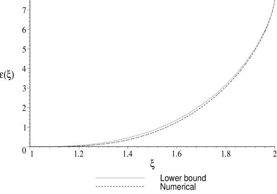
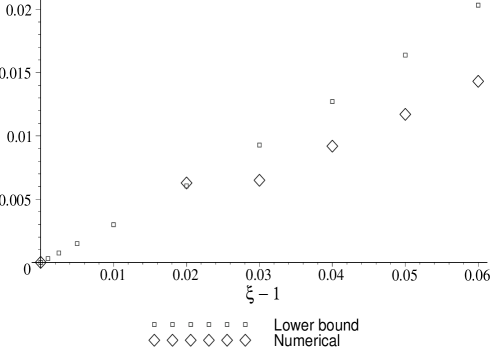
Figure 5: In the above figure we have plotted the lower bound $w_{0}$ with the numerical results of [14]. The middle figure shows plots of both data with $1/\log(\epsilon(\xi))^{2}$ on the y-axis. The lower bound data shows linear behavior consistent with the asymptotics in eq. (4.8). We note that there seems to be a numerical error in the data of [14] for $\xi=1.02$. In the lowest figure we have also plotted the numerical data in [14] near $\xi=2$ for $(15/2-\epsilon(\xi))^{3/2}$ showing linear behavior as expected in eq. 4.9. The plots in other dimensions look similar, except that they begin from the critical value $\xi^{*}>1$.

4.2 Asymptotics for $\xi$ near $\xi^{*}$ and 2

In this subsection we give estimates of the growth rate of the dynamo in the cases when $\xi$ is near the critical value $\xi^{*}$ above which dynamo is present, and when $\xi$ is near its maximum possible value 2. What we need is an estimate of the largest solution $w$ of Eq. (4.3), from which the corresponding growth rate $z$ is immediately deduced through Eq. (3.14). As an order of magnitude estimate for the solution, the simplest is to take the largest zero $w$ of $K_{\lambda}(w)$, as can be seen by inspecting Figure 4.

The case $\xi\searrow\xi^{*}$, corresponding to $\lambda\to 0$ along the imaginary axis, is somewhat simpler, it can be dealt with starting from the integral representation (4.7). Since $\xi>\xi^{*}$, the parameter $\lambda$ is imaginary and we write $\lambda=i\tilde{\lambda}$ with $\tilde{\lambda}\in\mathbb{R}$, hence $K_{i\tilde{\lambda}}(w)=\int_{0}^{\infty}dt\exp(-w\cosh(t))\cos(\tilde{\lambda}t)$. Now $\cos(\tilde{\lambda}t)$ is positive near $t=0$ and it becomes negative for the first time only for $t>\pi/(2\tilde{\lambda})$. On the other hand the term $\exp(-w\cosh(t))$ is basically a double exponential and decays very fast for $w\cosh(t)>1$. So in order to get for the previous integral a non-positive result, we need $w_{0}\cosh(\pi/(2\tilde{\lambda}))\sim 1$ implying $w_{0}\sim\exp(-\pi/(2\tilde{\lambda}))$. Through Eq. (3.14) one deduces the behaviour $\ln z\sim c/\tilde{\lambda}$, and since $\tilde{\lambda}\propto(\xi-\xi^{*})^{1/2}$ near $\xi^{*}$ (the term under the square root in Eq. (3.15) is expected to have a simple root at $\xi=\xi^{*}$), we finally have

$$\ln z\propto(\xi-\xi^{*})^{-1/2}$$ (4.8)

near $\xi^{*}$.

We now pass to the asymptotics of the case $\xi\to 2$. Under this limit $\lambda$ diverges as $(2-\xi)^{-1}$, along the complex axis. From plots or asymptotical formulae we can convience ourselves that the largest zero of $K_{\lambda}(w)$ occurs at $w\sim|\lambda|$, so that is the region where we are going to look for it. We write $K$ in terms of the Hankel function of first kind $K_{\lambda}(w)=\frac{i\pi}{2}e^{i\pi\lambda/2}H^{(1)}_{\lambda}(iw)$ and use the approximation formula in the transitory region (i.e. when parameter and argument of the Bessel function are of same order):

$$H^{(1)}_{\lambda}(\lambda+t\lambda^{1/3})\sim\frac{\sqrt{2}e^{i\pi/6}}{3\lambda^{1/3}t}H^{(1)}_{1/3}(\frac{\sqrt{8}}{3}t^{3/2})\,.$$

We deduce that there is some $t_{0}>0$ such that $w_{0}\sim|\lambda|-t_{0}|\lambda|^{1/3}=|\lambda|(1-t_{0}|\lambda|^{-2/3})$. Combining Eqs. (3.14) and (3.15) we get

$$z\approx z_{2}-c(2-\xi)^{2/3}\,,$$ (4.9)

valid for $\xi$ near 2, where $c>0$ is some constant of order unity and $z_{2}$ was introduced in Eq. (3.20).

4.3 Prandtl number $P\to\infty$

For large Prandtl number the analysis proceeds exactly as in the previous section, except that we have a different $\Lambda_{L}$. From Eqs. (B.47) and (B.44) we have, using the definition of $\zeta$ from Eq. (3.19),

$$\Lambda_{L} =\zeta-\frac{2}{d-1}-\frac{d}{2}\,.$$ (4.10)

There is now a branch cut originating from $z_{2}$ (defined in Eq. (3.20)) extending to infinity along the negative real axis. When $3\leq d\leq 8$, $z_{2}$ is positive and the branch cut extends up to the positive value $z_{2}$ along the positive real axis, i.e. the spectrum has a continuous positive part for all $\xi\in[0,2]$. Another major difference when comparing to the small Prandtl number case is that the spectrum is continuous also in the positive part.

We conclude that the dynamo is present for all $\xi$ for large Prandtl numbers.

5 Some remarks

5.1 Schrödinger operator formalism

We have performed our analysis in the diffusion process setting, but it could have equally well been done in the Schrödinger operator formalism (e.q. [14]), basically with the same kind of cutting up and piecing together technique.

Consider the zero energy Schrödinger equation

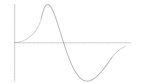
Figure 6: Sketchy plot of the medium range zero energy solution $\sin(\sqrt{1}5/2\log(r))$ crossing zero, implying the existence of a negative energy state. The dashed lines correspond to regions where the middle range approximation is no longer valid. As the range grows when increasing the Prandtl number, more zeros will emerge.

$$\psi^{\prime\prime}(r)=V(r)\psi(r),$$ (5.1)

where $V(r)=m(r)U(r)$ is the effective potential. The potential $V$ behaves as $2/r^{2}$ at very short and long scales, but as $-4/r^{2}$ at the medium range. The medium range solutions are $\sin(\sqrt{1}5/2\log(r))$ and $\cos(\sqrt{1}5/2\log(r))$. When the Prandtl number is increased, the medium range region is stretched, and it is clear that for sufficiently large Prandtl numbers the solutions cross zero an increasing number of times (see Fig. 6). According to a well known theorem, such a solution cannot be a ground state (see e.g. [12] pp. 90). In fact, the number of zeros of the solution (with nonzero derivative and excluding the zero at $r=0$) is the number of negative energy states, which implies the existence of unbounded growth.

5.2 Finite magnetic Reynolds number effects

Let us finally touch upon some questions not discussed in the text. Our method allows us in principle, without further complications, to estimate the critical magnetic Reynolds number (dependent on velocity roughness exponent $\xi$ and space dimension $d$) at which dynamo effect sets in, and the growth of the dynamo exponent with Reynolds number. However we get only a logarithmic estimate whose uncertainty is at least an order of magnitude or even two, which makes it not too useful. Notwithstanding, we would like to mention that the estimates we would obtain this way are hardly compatible with numerical results of [14], our thresholds being significantly lower. This issue is currently clarified with D. Vincenzi.

5.3 Exceptional solutions

An other issue is that of the existence of “exceptional” dynamos. It seems to us that the “typical” dynamo (note that we consider here only the infinte magnetic Reynolds number case) corresponds to the situation when our $\xi>\xi^{*}$, in which case there is an infinite discrete spectrum of growing modes. However our equations do not exclude a priori the possibility of a single growing mode at some $\xi<\xi^{*}$. In fact, if we take for example, at a formal level, $d=2.125$ then $\xi^{*}\approx 1.82$ and for $\xi^{\prime}\leq\xi<\xi^{*}$ (where $\xi^{\prime}$ is some value of which we only need to know here that $\xi^{\prime}<1.77$), Eq. (4.3) will have, in what we have called the small $z$ approximation (cf. Eq. (3.23)), a single solution $w_{0}>0$. If we take $\xi=1.77$ then $w_{0}\approx 0.077$ and $z\approx 8.8\cdot 10^{-5}\ll 1$ in a self-consistent manner. However it remains to be known if such a solution is not just an artefact of our resolution method, and if not, then to see if one can construct a model where such solutions occur for the more physical value of $d=3$.

6 Conclusions

The mean-field dynamo problem was considered in arbitrary space dimensions. We have shown that, to obtain the spectrum of the dynamo problem, the equation (4.3) has to be solved for $w$, from which the growth rate $z$ can be expressed through Eq. (3.14). The quantity $\Lambda_{L}$ appearing in Eq. (4.3) is given, for small magnetic Prandtl numbers, by either Eq. (4.4) or (4.6), depending on which of the self-consitent conditions (3.22) or (3.23) is verified (note that this leaves a gap between with no formula). For large magnetic Prandtl number we have to use Eq. (4.10) instead.

It was observed that, in our model, the dynamo can only exist when $3\leq d\leq 8$. The results for small Prandtl numbers were shown to confirm previous results [14, 9] obtained in three dimensions. For $d>3$ a critical value for $\xi$ was found, above which the dynamo is present, which is larger than the three dimensional critical value $\xi^{*}=1$. Furthermore, in the vanishing Prandlt number limit we have obtained the asymptotic estimates (4.8) and (4.9), which are in good qualitative agreement with numerical simulations of [14].

For large Prandtl numbers it was shown that the dynamo exists for all $\xi$ and that the spectrum is continuous. We hope our work will contribute to clarifying this somewhat controversial issue. The physical idea behind our explanations is that at large magnetic Prandtl number the magnetic field can feel the smooth scales of the fluid flow (they are not “wiped out” by magnetic diffusivity), and correlations in the velocity field above the magnetic diffusive scale $l_{\kappa}$ won’t do more harm to the dynamo than if we had a Batchelor type flow with no correlations of velocity at scales significantly larger than $l_{\kappa}$.

Our methods were based on approximating piecewise the evolution operator of the two point function of the magnetic field. This approximation introduces inaccuracies and one may ask how these influences the fine details of our reasoning, which relied on not so evident estimates. We think that the general picture sketched up should be valid for the exact problem also, based on the good agreement with available numerical data from the litterature. Since for $\xi=\xi^{*}$ and $\xi=2$ one can find the fastest growing mode explicitly, it should also be possible to do a perturbation theory around these points and place our results on a firmer ground. This is however left for future work.

7 Acknowledgements

H.A. would like to thank P. Muratore-Ginanneschi and A. Kupiainen for useful comments, suggestions and discussions related to the problem at hand. P.H. would like to thank A. Kupiainen for inviting him to work at the Mathematics Department of Helsinki University, where most of this work has been done. The work of H.A. was partly supported by the Vilho, Yrjö and Kalle Väisälä foundation. We would also like to thank Dario Vincenzi for discussing his results with us and providing data from his simulatons.

Appendix A PDE for the 2-point function of $\mathbf{B}$

We rewrite equation (1.1) as an Itô type SPDE (following the formalism of [10], sect. 5)

$$dB_{i}+d\mathbf{w}\cdot\nabla B_{i}-\mathbf{B}\cdot\nabla dw_{i}-\kappa^{\prime}\Delta B_{i}dt=0,$$ (A.1)

where $\kappa^{\prime}=\kappa+D/2$ with $D$ defined as

$$D_{ij}(0)=D\delta_{ij}.$$ (A.2)

The new diffusion term in $\kappa^{\prime}$ emerges by advecting the magnetic field along the particle trajectories similarly as in the passive scalar case by using the Itô formula. It will cancel out eventually, as it should. We can express the above equation more conveniently by defining

$$db_{i}(t,x)=-\mathcal{D}_{ijk}^{x}\left(B_{j}(t,x)dw_{k}(t,x)\right),$$ (A.3)

where $\mathcal{D}_{ijk}^{x}=\delta_{ij}\partial_{k}^{x}-\delta_{ik}\partial_{j}^{x}$ . The equation is then simply

$$dB_{i}-\kappa^{\prime}\Delta B_{i}dt=db_{i}.$$ (A.4)

For a function $F$ of fields $\mathbf{B}$, we have the (generalized) Itô formula,

$$dF\left(\mathbf{B}(t,\cdot)\right)=\!\int\!\!dx\frac{\delta F}{\delta B_{i}(x)}\left[\kappa^{\prime}\Delta B_{i}dt+db_{i}\right]+\frac{1}{2}\!\int\!\!dxdy\frac{\delta^{2}F}{\delta B_{i}(x)\delta B_{j}(y)}\mathbf{E}\left(db_{i}(t,x)db_{j}(t,y)\right).$$ (A.5)

The advecting velocity field is a time derivative of a Brownian motion on some state space, that is

$$\mathbf{E}dw_{i}(t,x)dw_{j}(t,y)=dtD_{ij}(x-y),$$ (A.6)

where $D_{ij}$ was defined in Eq. (1.3). This means that

$$\mathbf{E}db_{i}(t,x)db_{j}(t,y)=\mathcal{D}_{ikl}^{x}\mathcal{D}_{jmn}^{y}\left(u_{k}(t,x)u_{m}(t,y)D_{ln}(x-y)\right).$$ (A.7)

We apply this to $F=u_{i}(t,x)u_{j}(t,y)$, denote $G_{ij}(x-y)=\mathbf{E}u_{i}(t,x)u_{j}(t,y)$ and use the decomposition $D_{ij}(x-y)=D\delta_{ij}-d_{ij}(x-y)$ introduced in Eq. (1.5). Noting that terms proportional to $dw$ disappear, we obtain the equation for the two point function:

$$\frac{d}{dt}G_{ij}(t,\mathbf{r})=2\kappa\Delta G_{ij}(t,\mathbf{r})+\mathcal{F}_{ij},$$ (A.8)

where $\mathbf{r}=x-y$ and

$$\mathcal{F}_{ij}=d_{\alpha\beta}G_{ij,\alpha\beta}-d_{\alpha j,\beta}G_{i\beta,\alpha}-d_{i\beta,\alpha}G_{\alpha j,\beta}+d_{ij,\alpha\beta}G_{\alpha\beta}$$ (A.9)

where the indices after commas denote partial derivatives. Note that this depends only on $\kappa$, not $\kappa^{\prime}$, i.e. the constant part $D\delta_{ij}$ of the structure function is absent. Using the decomposition (1.11) and the explicit form of the long distance velocity structure function (1.7) we get from Eq. (A.8) two equations for $G_{1}$ and $G_{2}$,

$$\frac{dG_{1}}{dt}=\frac{2\kappa}{r^{2}}\left(2G_{2}+(d-1)rG_{1}^{\prime}+r^{2}G_{1}^{\prime\prime}\right)+\mathcal{A},$$ (A.10)

and

$$\frac{dG_{2}}{dt}=\frac{2\kappa}{r^{2}}\left(-2dG_{2}+(d-1)rG_{2}^{\prime}+r^{2}G_{2}^{\prime\prime}\right)+\mathcal{B}.$$ (A.11)

The symbols $\mathcal{A}$ and $\mathcal{B}$ are the terms arising from the interaction with the (long distance) velocity fields. Using the relations (1.15) for $G_{1}$ and $G_{2}$ in terms of $H$, their explicit form is as follows:

$$\frac{\mathcal{A}}{D_{1}r^{-2+\xi}} =\xi(d-1)(d-3+\xi)H(r)$$

$$\ldots +(2-d-2d^{2}+d^{3}+(-5+d+2d^{2})\xi+(1+d)\xi^{2})rH^{\prime}(r)$$

$$\ldots +(2d(d-1)+(d+1)\xi))r^{2}H^{\prime\prime}(r)+(d-1)r^{3}H^{\prime\prime\prime}(r),$$ (A.12)

$$-\frac{\mathcal{B}}{D_{1}r^{-2+\xi}} =-\xi(d-1)(2-\xi)H(r)$$

$$\ldots +((1-d^{2})+(d-5+2d^{2})\xi+4\xi^{2}-\xi^{3})rH^{\prime}(r)$$

$$\ldots +(d+1)(d-1+\xi)r^{2}H^{\prime\prime}(r)+(d-1)r^{3}H^{\prime\prime\prime}(r).$$ (A.13)

Now we can just add the equations (A.10) and (A.11), and by using $G_{1}+G_{2}=(d-1)H$ we get

$$\frac{dH}{dt} =\xi(d-1)(d+\xi)D_{1}r^{-2+\xi}H(r)$$

$$\ldots +\left(2(d+1)\kappa+(d^{2}-1+2\xi)D_{1}r^{\xi}\right)r^{-1}H^{\prime}(r)$$

$$\ldots +(2\kappa+(d-1)D_{1}r^{\xi})H^{\prime\prime}(r).$$ (A.14)

Appendix B Computation of the fraction $C_{L}^{-}/C_{L}^{+}$

By evaluating the matrix multiplications on the right hand side of Eq. (3.38), we can write the fraction $C_{L}^{-}/C_{L}^{+}$ as

$$\frac{C_{L}^{-}}{C_{L}^{+}}=-\frac{\partial h_{L}^{+}(1)-\Lambda_{L}h_{L}^{+}(1)}{\partial h_{L}^{-}(1)-\Lambda_{L}h_{L}^{-}(1)},$$ (B.1)

where $\Lambda_{L}$ can be written as the following nested expression:

$$\left\{\begin{array}[]{ll}\Lambda_{L}&=\frac{\partial h_{M}^{+}(1)+\Lambda_{M}\partial h_{M}^{-}(1)}{h_{M}^{+}(1)+\Lambda_{M}h_{M}^{-}(1)}\\ \Lambda_{M}&=-\frac{\partial h_{M}^{+}(a_{i})-\Lambda_{S}h_{M}^{+}(a_{i})}{\partial h_{M}^{-}(a_{i})-\Lambda_{S}h_{M}^{-}(a_{i})}\\ \Lambda_{S}&=\frac{\partial h_{S}(a_{i})}{h_{S}(a_{i})}.\end{array}\right.$$ (B.5)

This follows from defining

$$\begin{pmatrix}h_{S}\\ \partial h_{S}\end{pmatrix}_{a_{i}}=h_{S}(a_{i})\begin{pmatrix}1\\ \Lambda_{S}\end{pmatrix}$$ (B.6)

and writing equation (3.38) as

$$\begin{pmatrix}C_{L}^{+}\\ C_{L}^{-}\end{pmatrix}=c\begin{pmatrix}\partial h_{L}^{-}&\!\!\!-h_{L}^{-}\\ -\partial h_{L}^{+}&\!\!\!h_{L}^{+}\end{pmatrix}_{1}\begin{pmatrix}h_{M}^{+}&\!\!\!h_{M}^{-}\\ \partial h_{M}^{+}&\!\!\!\partial h_{M}^{-}\end{pmatrix}_{1}\begin{pmatrix}\partial h_{M}^{-}&\!\!\!-h_{M}^{-}\\ -\partial h_{M}^{+}&\!\!\!h_{M}^{+}\end{pmatrix}_{a_{i}}\begin{pmatrix}1\\ \Lambda_{S}\end{pmatrix},$$ (B.7)

where $h_{S}(a_{i})$ is absorbed in the coefficient. We have defined above a constant $c$ which gets cancelled in the end of computations. It will be used below as well as a generic constant that does not affect the final results. Multiplying the last matrix with the vector, we define similarly

$$\begin{pmatrix}\partial h_{M}^{-}&\!\!\!-h_{M}^{-}\\ -\partial h_{M}^{+}&\!\!\!h_{M}^{+}\end{pmatrix}_{a_{i}}\begin{pmatrix}1\\ \Lambda_{S}\end{pmatrix}=\begin{pmatrix}\partial h_{M}^{-}-\Lambda_{S}h_{M}^{-}\\ -\partial h_{M}^{+}+\Lambda_{S}h_{M}^{+}\end{pmatrix}_{a_{i}}=c\begin{pmatrix}1\\ \Lambda_{M}\end{pmatrix},$$ (B.8)

that is,

$$\Lambda_{M}=-\frac{\partial h_{M}^{+}(a_{i})-\Lambda_{S}h_{M}^{+}(a_{i})}{\partial h_{M}^{-}(a_{i})-\Lambda_{S}h_{M}^{-}(a_{i})}$$ (B.9)

Doing this again for the second matrix, we obtain similarly

$$\Lambda_{L}=\frac{\partial h_{M}^{+}(1)+\Lambda_{M}\partial h_{M}^{-}(1)}{h_{M}^{+}(1)+\Lambda_{M}h_{M}^{-}(1)}$$ (B.10)

and finally

$$\frac{C_{L}^{-}}{C_{L}^{+}}=-\frac{\partial h_{L}^{+}(1)-\Lambda_{L}h_{L}^{+}(1)}{\partial h_{L}^{-}(1)-\Lambda_{L}h_{L}^{-}(1)}.$$ (B.11)

We are interested in the leading order behavior of the fraction $C_{L}^{-}/C_{L}^{+}$ only, so we need to determine what happens to $\Lambda_{M}$ as $P$ approaches zero or infinity. It turns out that either $\Lambda_{M}\to 0$ or $\Lambda_{M}\to\pm\infty$, so to the leading order,

$$\Lambda_{L}=\frac{\partial h_{M}^{\pm}(1)}{h_{M}^{\pm}(1)}\ .$$ (B.12)

B.1 $P\ll 1$

Below the suspension dots denote higher order terms in powers of $P$ (or $P^{-1}$ for large Prandtl numbers). Recall from Eqs. (3.33) and (2.15) that

$$a_{1}=l_{\nu}/l_{\kappa}=\left(\frac{d-1}{2}P\right)^{1/\xi}.$$ (B.13)

The short range solution was

$$h_{S}(\rho)=\rho^{-d/2}\ I_{d/2}\left(\alpha\rho\right)$$ (B.14)

with a temporary notation $\alpha=\sqrt{(z+2P^{1-2/\xi}(2-d-d^{2}))/(d-1)}$ and note that $|\alpha|$ behaves as $P^{1/2-1/\xi}$. Using standard relations of Bessel functions [7] and using the definition for $\Lambda_{S}$ in Eq. (B.5), we have

$$\Lambda_{S}=\frac{\partial h_{S}(a_{1})}{h_{S}(a_{1})}=\alpha\frac{I_{1+d/2}\left(\left(\frac{d-1}{2}P\right)^{1/\xi}\alpha\right)}{I_{d/2}\left(\left(\frac{d-1}{2}P\right)^{1/\xi}\alpha\right)}.$$ (B.15)

Since $P$ is small and the arguments of the Bessel functions above scale as $P^{1/2}$, we can use the expansion

$$I_{d/2}(u)=u^{d/2}\left(\frac{2^{-{d/2}}}{\Gamma(1+d/2)}+\frac{2^{-2-d/2}}{\Gamma(2+d/2)}u^{2}+\mathcal{O}(u^{4})\right)$$ (B.16)

(and a corresponding one when the order parameter is $1+d/2$) to conclude that

$$\Lambda_{S}=cP^{1-1/\xi}+\ldots$$ (B.17)

The medium range solutions in the large $z$ case, Eq. (3.24), are

$$h_{M,1}^{\pm}(\rho)=\rho^{-d/2}\left\{\begin{array}[]{cc}I_{d/2}&\\ K_{d/2}&\end{array}\right.\!\!\!\!\!\!\!\!\!\left(\sqrt{\beta}\rho\right),$$ (B.20)

with $\beta=z/(d-1)$. The leading order behavior is

$$\left\{\begin{array}[]{ll}h_{M}^{+}(a_{1})&=c+\ldots\\ \partial h_{M}^{+}(a_{1})&=cP^{1/\xi}+\ldots\\ h_{M}^{-}(a_{1})&=cP^{-d/\xi}+\ldots\\ \partial h_{M}^{-}(a_{1})&=cP^{-1/\xi-d/\xi}+\ldots\end{array}\right.$$ (B.25)

Using these on $\Lambda_{M}$ as given by Eq. (B.9), we see that to leading order

$$\Lambda_{M}=cP^{d/\xi+1},$$ (B.26)

which goes to zero. Therefore we have

$$\Lambda_{L}\sim\frac{\partial h_{M}^{+}(1)}{h_{M}^{+}(1)}=\sqrt{\frac{z}{d-1}}\frac{I_{1+d/2}\left(\sqrt{\frac{z}{d-1}}\right)}{I_{d/2}\left(\sqrt{\frac{z}{d-1}}\right)}.$$ (B.27)

Note that, notwithstanding the fractional powers appearing above, $\Lambda_{L}$ is a single valued function, indeed near $z=0$ it behaves as $\Lambda_{L}\approx z/(d-1)$. One also notes that in the large $z$ case $\Lambda_{L}$ is always positive, since the Bessel functions $I$ are positive for positive parameter and argument.

We may perform a similar analysis for the small $z$ approximation, based on Eq. (3.25),

$$h_{M,1}^{\pm}(\rho)=\rho^{-d/2}\left\{\begin{array}[]{cc}J_{d/\xi}&\\ Y_{d/\xi}&\end{array}\right.\!\!\!\!\!\!\!\!\!\left(\gamma\rho^{\xi/2}\right),$$ (B.30)

with $\gamma=2\sqrt{d/\xi+1}$. The leading order behavior is

$$\left\{\begin{array}[]{ll}h_{M}^{+}(a_{1})&=c+\ldots\\ \partial h_{M}^{+}(a_{1})&=cP^{1-1/\xi}+\ldots\\ h_{M}^{-}(a_{1})&=cP^{-d/\xi}+\ldots\\ \partial h_{M}^{-}(a_{1})&=cP^{-1/\xi-d/\xi}+\ldots\end{array}\right.$$ (B.35)

Using these on $\Lambda_{M}$ (cf. Eq. (B.9)), we see that once again $\Lambda_{M}$ behaves at leading order as given in Eq. (B.26), meaning that it goes to zero as $P$ goes to zero. Therefore we have

$$\Lambda_{L}\sim\frac{\partial h_{M}^{+}(1)}{h_{M}^{+}(1)}=-\xi\sqrt{d/\xi+1}\frac{J_{d/\xi+1}(2\sqrt{d/\xi+1})}{J_{d/\xi}(2\sqrt{d/\xi+1})}\,.$$ (B.36)

In the particular case of $\xi=2$ the medium range solution can be explicitly calculated for any $z$, and we have

$$h_{M,1}^{\pm}(\rho)=\rho^{-d/2}\left\{\begin{array}[]{cc}J_{d/2}&\\ Y_{d/2}&\end{array}\right.\!\!\!\!\!\!\!\!\!\left(\sqrt{\beta}\rho\right)\,,$$ (B.39)

where now $\beta=2(d+2)-z/(d-1)$. The approximations in Eq. (B.25) or (B.35) (for $\xi=2$ those two coincide) are valid unfiromly as $\xi$ goes to 2, so when $\beta$ is of order unity, the leading order behaviour Eq. (B.26) is valid. Note that for $z=z_{2}$ we indeed have $\beta$ of order unity. Now one deduces that $\Lambda_{L}=-\sqrt{\beta}J_{d/2+1}(\sqrt{\beta})/J_{d/2}(\sqrt{\beta})$, and for $z=z_{2}$ one finds $\sqrt{\beta}=(d^{2}-d+4)/4/(d-1)$. One can then verify numerically that for $\xi=2$ and $z=z_{2}$ and relevant values of $d$ (between 3 and 8 inclusive) we have $\tilde{\Lambda}_{L}>0$. By continuity, positivity carries over to values of $\xi$ close to 2 and the corresponding dynamo growth rate $z$. This permits us to use near $\xi=2$ the upper bound $w_{0}^{\prime}$ on the largest solution of Eq. (4.3), and obtain the asymptotic behaviour of Sect. 4.2.

B.2 $P\gg 1$

Now we have $a_{2}=\left((d-1)P/2\right)^{-1/2}$. The short range solution is in this case

$$h_{S}(\rho)=\rho^{-d/2}\ I_{d/2}\left(\sqrt{P}\alpha^{\prime}\rho\right)$$ (B.40)

with

$$\alpha^{\prime}=\frac{1}{\sqrt{2}}\sqrt{z+2(2-d-d^{2})}.$$ (B.41)

Similarly to the $P\ll 1$ case,

$$\Lambda_{S}=\sqrt{P}\alpha^{\prime}\frac{I_{1+d/2}(\sqrt{\frac{2}{d-1}}\alpha^{\prime})}{I_{d/2}(\sqrt{\frac{2}{d-1}}\alpha^{\prime}))}=c\sqrt{P}+\ldots$$ (B.42)

The medium range solutions are now power laws,

$$h_{M}^{\pm}=\rho^{-d/2-2/(d-1)\pm\delta},$$ (B.43)

where

$$\delta=\frac{\sqrt{d(d^{3}-10d^{2}+9d+16)+4(d-1)z}}{2(d-1)}.$$ (B.44)

Since $\partial h_{M}^{\pm}(a_{2})\propto\sqrt{P}h_{M}^{\pm}(a_{2})$,

$$\partial h_{M}^{\pm}(a_{2})-\Lambda_{S}h_{M}^{\pm}(a_{2})=c\sqrt{P}h_{M}^{\pm}(a_{2})+\ldots,$$ (B.45)

that is,

$$\Lambda_{M}=c\frac{h_{M}^{+}(a_{2})}{h_{M}^{-}(a_{2})}+\ldots=c\frac{1}{P}+\ldots.$$ (B.46)

This goes to zero as $P\to\infty$, and we have

$$\Lambda_{L}\to\frac{\partial h_{M}^{+}(1)}{h_{M}^{+}(1)}=\zeta-\frac{2}{d-1}-\frac{d}{2}.$$ (B.47)

where $\zeta$ was defined in Eq. (3.19). In fact we wouldn’t have needed to worry if the limit of $\Lambda_{M}$ was infinite or zero. The difference would only be a different sign of $\zeta$, which doesn’t affect anything since it is the presence of the branch cut alone which determines the positive part of the spectrum.

Appendix C Some Sturm-Liouville theory

Consider the following general second order linear eigenvalue problem, where $a,b,c$ are positive functions and $z\in\mathbb{R}$:

$$a(\rho)h^{\prime\prime}(\rho)+b(\rho)h^{\prime}(\rho)+c(\rho)h(\rho)=zh(\rho)\,.$$ (C.1)

Introduce $g=h^{\prime}/h$, then $g$ verifies the first order non-linear (Riccati) differential equation

$$g^{\prime}=\frac{z-c-bg-ag^{2}}{a}\,.$$ (C.2)

Note that a zero of $h$ corresponds to a pole of $g$, and the pole is always such that as $\rho$ increases $g$ goes to $-\infty$ and comes back at $+\infty$ (since if $h$ is positive before crossing zero then its derivative must be negative and vice versa).

C.1 Montonicity of solutions in $z$

Consider for Eq. (C.1) the initial condition $h^{\prime}(0)=0$ and $h(0)>0$ which in particular implies $g(0)=0$. Now consider Eqs. (C.1) and (C.2) for two different values of $z$, say $z_{1}$ and $z_{2}$, and denote the corresponding solutions by $h_{1}$, $g_{1}$ and $h_{2}$, $g_{2}$ respectively. We show that if $z_{1}>z_{2}$, then $g_{1}(\rho)>g_{2}(\rho)$ for $\rho$ less than the first zero of $h_{2}$.

This can be seen as follows. First, the assertion is true near $\rho=0$ since $g_{1}^{\prime}(0)=(z_{1}-c(0))/a(0)>(z_{2}-c(0))/a(0)=g_{2}^{\prime}(0)$ while $g_{1}(0)=g_{2}(0)=0$. Now suppose that at some point the ordering of $g_{1}$ and $g_{2}$ changes, this means that the two have to cross, i.e. for some $\rho$ we have $g_{1}(\rho)=g_{2}(\rho)=G$. However at this point $g_{1}^{\prime}(\rho)=(z_{1}-c(\rho)-b(\rho)G-a(\rho)G^{2})/a(\rho)>(z_{2}-c(\rho)-b(\rho)G-a(\rho)G^{2})/a(\rho)=g_{2}^{\prime}(\rho)$, meaning that $g_{1}$ cannot cross $g_{2}$ downwards, which is a contradiction.

Application 1

From the above it also follows that the first zero of $h_{1}$ is larger than the first zero of $h_{2}$. Indeed $h_{2}$ has no zero before its first zero, so $g_{2}$ doesn’t go to $-\infty$ before that point, implying that $g_{1}$ neither since $g_{1}>g_{2}$, thus $h_{1}$ has no zero either before the first zero of $h_{2}$.

A particularly useful application of this is to use the position of the first zero of the solution with $z=0$ as a lower bound on the first zero of any solution for $z>0$.

Application 2

We may apply the above to the case when Eq. (C.1) is taken to be Eq. (2.17b). For $P\to 0$ the intial condition at $\rho=0$ becomes $h_{M}^{\prime}=0$. The case $z=0$ can be explicitly solved and we get $h_{M}(\rho)=\rho^{-d/2}J_{d/\xi}(2\sqrt{d/\xi+1}\,\rho^{\xi/2})$. What needs to be seen is that $h_{M}$ does not have zeros between 0 and 1, equivalent to $J_{d/\xi}$ not having zeros between 0 and $2\sqrt{d/\xi+1}$, which follows from the fact that $j_{\nu,1}>2\sqrt{\nu+1}$ for $\nu\geq 0$ (where $j_{\nu,1}$ is the first positive zero of the Bessel function of index $\nu$), which may be easily verified by a plot or by more serious analysis. We remark that $h_{M}^{\prime}$ does have zeros, as an effect of the term $\xi(d-1)(d+\xi)\rho^{\xi-2}h_{M}$ in Eq. (2.17b), and thus the fact that $\Lambda_{L}$ is indeed monotonously increasing is surprisingly non trivial because of this term.

All this allows us to conclude that $\Lambda_{L}=h_{M}^{\prime}(1)/h_{M}(1)$ grows with $z$ (equivalently with $w$).

Application 3

Along the same lines one can prove for our case the standard lore of Sturm-Liouville theory that if the zero mode ($z=0$ solution) has no zeros, then there is no eigenfunction with $z>0$.

The idea is that while the zero mode decays near infinity as a power law, any eigenfunction $h_{1}$ for $z>0$ has to decay exponentially, so it will be below the zero mode. On the other hand, from Eq. (C.1) on deduces that $h^{\prime\prime}(0)$ grows with $z$, so that $h_{1}$ has to be larger than the zero mode near $\rho=0$. This would imply that the two have to cross in the sense that $h_{2}$ comes from above and goes below the zero mode, but at the crossing point $g_{1}$ would be less than that of the zero mode, which contradicts the above said.

C.2 Consequences for modified Bessel function

We wish to prove here that, for pure imaginary $\lambda$, the slope of $\rho K^{\prime}_{\lambda}(\rho)/K_{\lambda}(\rho)$ is bounded from above by $-1$ for all $\rho>0$.

Using notation from the previous subsections, introduce $f(\rho)=\rho g(\rho)$. Then Eq. (C.2) translates to $f^{\prime}=[(z-c)\rho+(a/\rho-b)f-(a/\rho)f^{2}]/a$. Applied to the particular case of the modified Bessel equation with parameter $\lambda$

$$\rho^{2}h^{\prime\prime}+\rho h^{\prime}-\rho^{2}h=\lambda^{2}h\,,$$

i.e. when $a(\rho)=\rho^{2}$, $b(\rho)=\rho$, $c(\rho)=-\rho^{2}$ and $z=\lambda^{2}$, we obtain

$$f^{\prime}=(\rho^{2}+\lambda^{2}-f^{2})/\rho\,.$$ (C.3)

Solving Eq. (C.3) for $f^{\prime}=-1$ gives $f^{2}=s(\rho)^{2}$ where we define $s(\rho)=-[(\rho+1/2)^{2}+\lambda^{2}-1/4]^{1/2}$. Moreover when $f^{2}>s^{2}$ then $f^{\prime}<-1$.

We now take $f=\rho K^{\prime}_{\lambda}(\rho)/K_{\lambda}(\rho)$ in the case when $\lambda$ is pure imaginary. Then, for large $\rho$, asymptotically $f(\rho)-s(\rho)\sim-(1-4\lambda^{2})/(16\rho^{2})<0$, the last inequality being guaranteed by the fact that we consider the case when $\lambda$ is pure imaginary and hence $\lambda^{2}\leq 0$. This means that for large $\rho$ asymptotically $f<s$.

Using the fact that $f$ is continuous, if $f$ were to become larger than $s$ for some finite $\rho$, necessarily it would pass through $f=s$, but at that point we would have $f^{\prime}=-1>s^{\prime}$ (the inequality holding for $\lambda$ pure imaginary), which is a contradiction to the fact that for larger $\rho$ we should have $f<s$.

This proves that $f<s\leq 0$ when $s$ is real, and thus $f^{2}>s^{2}$ for all $\rho\geq 0$, whence $f^{\prime}<-1$ for $\rho\geq 0$.

C.3 Real spectrum

Though we do not consider $\mathcal{M}$ to be self-adjoint, its spectrum is always real, for the following reason.

Since $\mathcal{M}$ is a second order differential operator we may conjugate it by a multiplication operator (by a “function” which is known in the thory of diffusion processes as the speed measure) to get a symmetric operator $\tilde{\mathcal{M}}$, and taking into account the boundary conditions we have (we see that for any $z\in{\mathbb{C}}\setminus{\mathbb{R}}_{-}$ the solution of $\tilde{\mathcal{M}}h=zh$ which verifies the boundary conditions is a twice differentiable function with zero derivative at $\rho=0$ and exponentially decaying as $\rho\to\infty$, so $h$ is also in the domain of $\tilde{\mathcal{M}}^{\dagger}$), we can use the same trick as for self-adjoint operators: suppose $\tilde{\mathcal{M}}h=zh$ and write $\int\bar{h}\tilde{\mathcal{M}}h=z\int\bar{h}h$, now take the complex conjugate of both sides, and since $\tilde{\mathcal{M}}$ is real and symmetric, we have $\int\bar{h}\tilde{\mathcal{M}}h=\bar{z}\int\bar{h}h$, showing that $z=\bar{z}$, i.e. that $z$ is real.

Appendix D Exact results for $P=0$

Here we want to study more rigorously the case of $P=0$. In this case we can find exactly the zero mode of Eq. (2.9) and show that for $\lambda$ real (recall its definition from Eq. (3.15)) it has no nodes. On the other hand for $\lambda$ pure imaginary it has an infinity of nodes.

Recalling Eq. (2.13), first we have to solve the zero mode equation $[\xi(d-1)(d+\xi)\rho^{\xi-2}+(d^{2}-1+2\xi)\rho^{\xi-1}\partial_{\rho}+(d-1)\rho^{\xi}\partial_{\rho}^{2}]+[(d^{2}-1)\rho^{-1}\partial_{\rho}+(d-1)\partial_{\rho}^{2}]$. At 0 Prandtl number the boundary condition is to have finite limit at $\rho=0$. The appropriate solution is

$$(\rho^{\xi}+1)^{(d-3)/(d-1)}{}_{2}F_{1}\left(\begin{array}[]{c}\frac{2(d-2)\xi+d(d-1)+(2-\xi)(d-1)\lambda}{2\xi(d-1)},\frac{2(d-2)\xi+d(d-1)-(2-\xi)(d-1)\lambda}{2\xi(d-1)}\\[8.61108pt] \frac{d+\xi}{\xi}\end{array};-\rho^{\xi}\right)$$

where ${}_{2}F_{1}$ is the hypergeometric function, which we shall simply denote as ${}_{2}F_{1}(a,b;c;x)$, and $a,b,c,x$ are defined accordingly to the above displayed formula.

Let us start with the case of $\lambda$ real. Without loss of generality, we may suppose $\lambda>0$ (or otherwise exchange $a$ and $b$, since the hypergeometric function is symmetric in those arguments). Notice that $2(d-2)\xi+d(d-1)>0$ and $[2(d-2)\xi+d(d-1)]^{2}-[(2-\xi)(d-1)\lambda]^{2}=2d^{2}(d-1)^{2}-8\xi^{2}(d-2)\geq 2[d^{2}(d-1)^{2}-16(d-2)]>0$, implying $b>0$.

Notice also $2(d-1)(d+\xi)-[2(d-2)\xi+d(d-1)]=d(d-1)+2\xi>0$ implying $c-b>0$.

Now write the following integral representation of the hypergeometric function:

$${}_{2}F_{1}(a,b;c;x)=\frac{\Gamma(c)}{\Gamma(b)\Gamma(c-b)}\int_{0}^{1}\frac{t^{b-1}(1-t)^{c-b-1}}{(1-tx)^{a}}\,dt\qquad(c>b>0)$$

whence ${}_{2}F_{1}(a,b;c;x)>0$ for any $x<1$ and $c>b>0$.

Since we have shown above $c>b>0$ and since our $x<0$, this proves that the zero mode has no zeros, and hence there cannot be a dynamo effect.

For $\lambda$ pure imaginary it is possible to make a large $\rho$ development using the so called linear transformation formula ${}_{2}F_{1}(a,b;c;-x)=\frac{\Gamma(c)\Gamma(b-a)}{\Gamma(b)\Gamma(c-a)}x^{-a}{}_{2}F_{1}(a,1-c+a;1-b+a;-1/x)+\frac{\Gamma(c)\Gamma(a-b)}{\Gamma(a)\Gamma(c-b)}x^{-b}{}_{2}F_{1}(b,1-c+b;1-a+b;-1/x)$. Since $a$ and $b$ are complex conjugates in the case of pure imaginary $\lambda$, the large $x$ asymptotics can be written as ${}_{2}F_{1}(a,b;c;-x)\sim\Re(\frac{\Gamma(c)\Gamma(b-a)}{\Gamma(b)\Gamma(c-a)}x^{-a})$, which has an infinity of zeros since $a$ has an imaginary part.

References

- [1] L. Ts. Adzhemyan, N.V. Antonov, A. Mazzino, P. Muratore-Ginanneschi, A.V. Runov, “Pressure and intermittency in passive vector turbulence”, Europhys. Lett. 55 (6):801 (2001), arXiv:nlin/0102017
- [2] K-J. Engel, R. Nagel, “One-Parameter Semigroups for Linear Evolution Equations”, Springer-Verlag, 2000
- [3] G. Falkovich, K. Gawedzki, M. Vergassola, “Particles and Fields in Fluid Turbulence”, Rev. Mod. Phys., Vol. 73, pp. 913–975, 2001
- [4] K. Gawedzki, A. Kupiainen, “Universality in Turbulence: an Exactly Soluble Model”, In:Low-dimensional models in statistical physics and quantum field theory. H. Grosse and L. Pittner (eds.), Springer, Berlin 1996, pp. 71–105, arXiv:chao-dyn/9504002
- [5] K. Gawedzki, P. Horvai, “Sticky behavior of fluid particles in the compressible Kraichnan model” J. Stat. Phys. vol. 116, no. 5-6, September 2004, pp. 1247–1300(54)
- [6] R.J. Goldston, P.H. Rutherford, “Introduction to Plasma Physics”, IOP Publishing, 1995
- [7] I.S. Gradshteyn, I.M. Ryzhik, “Table of Integrals, Series and Products”, Academic Press, 1965
- [8] V. Hakulinen, “Passive Advection and the Degenerate Elliptic Operators ”, Comm.Math.Phys., Vol. 235, Issue 1, Apr 2003, pp. 1–45 , arXiv:math-ph/0210001; Y. Le Yan, O. Raimond, “Integration of Brownian vector fields”, Ann. Probab. 30, no. 2 (2002), 826–873, arXiv:math.PR/9909147
- [9] A.P.Kazantsev, “Enhancement of a magnetic field by a conducting fluid flow”, Sov. Phys. JETP, 26, 1031 (1968)
- [10] A. Kupiainen, “Statistical Theories of Turbulence”, Lecture notes from “Random Media 2000”, Madralin, June 2000, http://www.helsinki.fi/~ajkupiai/papers/poland.ps
- [11] A. Lunardi, “Analytic Semigroups and Optimal Regularity in Parabolic Problems”, Birkhäuser, 1995
- [12] M. Reed, B. Simon, “Methods of Modern Mathematical Physics IV: Analysis of Operators”, Academic Press, 1978
- [13] M. Vergassola “Anomalous scaling for passively advected magnetic fields”, Phys. Rev. E 53, R3021–R3024 (1996)
- [14] D. Vincenzi, “The Kraichnan-Kazantsev Dynamo”, J. Stat. Phys. Vol. 106, Nos. 516, March 2002
- [15] D. Vincenzi (private communication)
- [16] G.N. Watson, “Theory of Bessel Functions”, Cambridge University Press, 1962