Nonlinear dynamics and chaos Classical transport

Peeping at chaos: Nondestructive monitoring of chaotic systems by measuring long-time escape rates

Abstract

One or more small holes provide non-destructive windows to observe corresponding closed systems, for example by measuring long time escape rates of particles as a function of hole sizes and positions. To leading order the escape rate of chaotic systems is proportional to the hole size and independent of position. Here we give exact formulas for the subsequent terms, as sums of correlation functions; these depend on hole size and position, hence yield information on the closed system dynamics. Conversely, the theory can be readily applied to experimental design, for example to control escape rates.

A fundamental issue in physical measurement (whether classical or quantum) is ensuring that the system to be studied is little affected by the observation. This is clearly much easier to satisfy if the measuring device lies outside the system. A truly isolated system cannot affect its surroundings, and is impossible to observe. However it can be to a good approximation unaffected by a very small hole, through which particles or radiation can carry information about the internal dynamics. Notice that theory and experiment often work in opposite directions: theorists use closed systems to understand open ones, while experimentalists do the reverse.

The initial motivation for this work came from atom-optics billiards [1, 2] in which escape properties were used to distinguish regular and chaotic behavior, but for which a detailed theory was absent, a deficit which the current work aims to address. Our theory is however far more general than these experiments suggest; billiards in which a particle moves in straight lines making specular reflections with a boundary are relevant to any system with particles in a relatively homogeneous cavity. Experimental realizations have included microwaves [3, 4, 5, 6], visible light [7], phonons in quartz blocks [8], and electrons in semiconductors [9, 10]. Furthermore, transport through small holes (in phase space) has applications as diverse as the transition state theory of chemical reactions [11], the migration of asteroids [12], and passive advection in fluids [13]. It can also help to characterise chaos in relativity [14] and in Hamiltonian systems in general [15]. Finally, the “hole” can be a desired region in phase space, for example a set from which we can subsequently control the dynamics with small perturbations; the escape rate then gives information on how long we may need to wait before attempting control [16]. We emphasize that while our numerical example is a billiard, the method is readily applicable to general volume preserving (for example Hamiltonian) systems.

Just as black body radiation emanating from a cavity through a small hole gives only a single piece of information (the temperature), we would expect the transport properties of orbits in the phase space of open systems to give only simple geometrical information to leading order. The transit time (for orbits entering through a hole then exiting) is exactly given by the ratio of hole to system sizes [17]. The escape rate (for orbits initially in the system) is hard to characterize in general [18], but is also often assumed to follow a similar equation [17]. In a previous Letter [19], we showed a result of this type for the regular circle billiard, with corrections computed analytically. Stadium and related billiards with interior holes have also been studied recently [20]. Here we consider general strongly chaotic systems in the limit of small holes, and find an analytic expansion of the escape rate, in which the ratio of hole and system sizes gives the leading term, and corrections are given by correlation functions. Measurement of the escape rate of a hole as a function of size and position, or of two holes compared to the individual escape rates, then provides a window through which to study the original (closed) dynamics.

The use of correlation functions to compute transport coefficients is familiar from Green-Kubo formulas [21]. Also, the escape rate from rather specific systems of large spatial extent can be used to compute general transport coefficients [22]. Thus the appearance of correlation functions in more general escape rate calculations should not come as a surprise. We also note that the periodic orbit formalism for computation of escape rates of open chaotic systems [23, 24] is unsuitable for the limit of small holes, as a very large number of periodic orbits would be required for the hole(s) to be sufficiently covered.

Our formalism is in the setting of volume preserving maps $\Phi:M\to M$, such as Hamiltonian evolution considered at equally spaced times (a “stroboscopic map”) or when a certain condition is met (a “Poincaré map”). We use $\langle f\rangle$ to denote an integral of a phase variable $f:M\to\mathbb{R}$ over the normalised volume element of the phase space $M$. Even when the dynamics does not preserve the usual volume (for example leading to a strange attractor), there is often a well defined fractal measure which is preserved, albeit making calculations of correlation functions more complicated.

A particular case of a Poincaré map is that of a billiard system of a particle moving uniformly between specular collisions with the boundary $\partial D$ of a two dimensional domain $D$, where $\Phi$ denotes the evolution from one collision to the next. In this case the phase space volume element of the flow projects to the area element $dldp_{\parallel}$ of $M$ preserved under $\Phi$, where $l$ measures arc length along the boundary and $p_{\parallel}$ is the component of momentum parallel to the boundary after the collision. Thus for a phase function $f$ on the billiard boundary we have

$$\langle f\rangle=\frac{\int f(l,p_{\parallel})dldp_{\parallel}}{\int dldp_{\parallel}}$$ (1)

where the denominator is simply $2|{\bf p}||\partial D|$.

We now return to the general formalism and define some phase variables on $M$. Let the function $T:M\to\mathbb{R}$ denote the time from one collision to the next; this is necessary to relate collision number with real time $t$. We assume this function is bounded from above. The holes are represented by a characteristic function $\chi:M\to\mathbb{R}$ equal to zero on a hole and one elsewhere; in the billiard example this is normally a function only of $l$ and not $p_{\parallel}$. Note that our approach here is to always use the dynamics of the closed system, but “kill” escaping trajectories using a multiplication by $\chi$. $\langle\chi\rangle\equiv 1-h$ is simply the fraction of $M$ not covered by holes and $h$ is the size of the hole (relative to $|M|$). Another useful set of averages is $\tau_{k}\equiv\langle T^{k}\chi\rangle/\langle\chi\rangle$, the average of the $k$th power of the collision time over the non-hole part of the system. We will need a weighted characteristic function $\chi_{s}:M\to\mathbb{R}$ defined by $\chi_{s}\equiv e^{sT}\chi$, so that $\chi_{0}=\chi$. It is also useful to define phase functions with averages subtracted; we find that the best way to do this is to set $\hat{\chi}_{s}\equiv\chi_{s}/\langle\chi_{s}\rangle-1$ so that $\hat{\chi}=\hat{\chi}_{0}=\chi/\langle\chi\rangle-1$. We also define $\hat{T}\equiv T-\tau_{1}$ and $\hat{\tau}_{k}=\langle\hat{T}^{k}\chi\rangle/\langle\chi\rangle$.

Assume that the phase space is filled with initial conditions (or mutually non-interacting particles) of a uniform density with respect to the preserved volume element, then consider the survival probability $P(t)$ for time $t$, so $P(0)=1$. The exponential escape rate $\gamma$, defined for strongly chaotic systems, is

$$\gamma=-\lim_{t\to\infty}\frac{\ln P(t)}{t}$$ (2)

which is well behaved in strongly chaotic systems and is equal to the leading pole (that is, of smallest $s>0$) of the function

$$\int_{0}^{\infty}e^{st}P(t)dt=\int_{0}^{\infty}e^{st}\langle\chi^{0}\chi^{1}\ldots\chi^{N_{t}}\rangle dt$$ (3)

where $N_{t}$ is the number of collisions before time $t$ and a superscript on a phase variable from now on will usually denote discrete time, ie $\chi^{j}\equiv\chi\circ\Phi\circ\cdots\circ\Phi$, with the map $\Phi$ composed $j$ times. We can rewrite this as

$$\int_{0}^{\infty}\langle\chi^{0}_{s}\chi^{1}_{s}\ldots\chi^{N_{t}}_{s}\rangle dt=\sum_{N=0}^{\infty}\langle\chi^{0}_{s}\chi^{1}_{s}\ldots\chi^{N}_{s}T^{N}\rangle$$ (4)

where $\chi_{s}$ is defined above, and we have ignored a factor bounded in magnitude which does not affect the leading pole. Now assuming that the long time escape is not dominated by orbits with very small $T$ (hence $T^{N}$ is also effectively bounded), the escape rate is given by the leading pole of

$$G(s)=\sum_{N=0}^{\infty}G_{N}(s)=\sum_{N=0}^{\infty}\langle\chi^{0}_{s}\chi^{1}_{s}\ldots\chi^{N}_{s}\rangle$$ (5)

Substituting $\chi_{s}=\langle\chi_{s}\rangle(1+\hat{\chi}_{s})$ to isolate the leading part, and then expanding and grouping into terms with different numbers of $\hat{\chi}_{s}$, we find

$$G(s)=\sum_{N=0}^{\infty}\langle\chi_{s}\rangle^{N+1}\Gamma_{N}(s)$$ (6)

where

$$\Gamma_{N}(s) = \sum_{n=0}^{N+1}\sum_{0\leq j_{1}<j_{2}\ldots<j_{n}\leq N}\langle\hat{\chi}_{s}^{j_{1}}\hat{\chi}_{s}^{j_{2}}\ldots\hat{\chi}_{s}^{j_{n}}\rangle$$

$$= 1+\sum_{0\leq j<k\leq N}\langle\hat{\chi}_{s}^{j}\hat{\chi}_{s}^{k}\rangle+\sum_{0\leq j<k<l\leq N}\langle\hat{\chi}_{s}^{j}\hat{\chi}_{s}^{k}\hat{\chi}_{s}^{l}\rangle+\ldots$$

Remarks:

1. The single sum ($n=1$) is absent since the average of $\hat{\chi}_{s}$ is zero by definition.

2. This expansion is divergent since the number of terms in each sum gets larger with each term, and the higher order correlations are small but finite.

The sum for $G(s)$ diverges when the ratio of subsequent terms exceeds unity in the limit, so at the first zero of

$$g(s)\equiv\lim_{N\to\infty}g_{N}(s)$$ (8)

where

$$g_{N}(s)=\ln\frac{G_{N+1}(s)}{G_{N}(s)}=\ln\langle\chi_{s}\rangle+\ln\Gamma_{N+1}(s)-\ln\Gamma_{N}(s)$$ (9)

Expanding the logarithms and taking the limit, we find

$$g(s)=\ln\langle\chi_{s}\rangle+\sum_{n=2}^{\infty}Q_{n}(s)$$ (10)

where the cumulants $Q_{n}(s)$ are

$$Q_{2}(s) = \sum_{0<j}\langle\hat{\chi}_{s}^{0}\hat{\chi}_{s}^{j}\rangle$$

$$Q_{3}(s) = \sum_{0<j<k}\langle\hat{\chi}_{s}^{0}\hat{\chi}_{s}^{j}\hat{\chi}_{s}^{k}\rangle$$ (11)

The higher cumulants are more complicated, for example $Q_{4}(s)$ includes 4-time correlations and products of 2-time correlations. We expect this cumulant expansion (by analogy with [25]) to be well defined if the system has multiple correlation functions decaying faster than any power (which, a posteriori, is what we mean by “chaotic”). Decay with a power greater than unity will permit $Q_{2}(s)$ to exist, and hence allow the second order formulas below to be used.

We are interested in the limit of small holes, ie small escape rate. Thus we expand these quantities in powers of $s$:

$$\hat{\chi}_{s} = \hat{\chi}+(1+\hat{\chi})\left[s\hat{T}+\frac{s^{2}}{2}\left(\hat{T}^{2}-\hat{\tau}_{2}\right)+\ldots\right]$$ (12)

Note that the first term is independent of $s$ and the remainder is projected onto the non-hole part by $1+\hat{\chi}$.

$$\ln\langle\chi_{s}\rangle=\ln\langle\chi\rangle+s\tau_{1}+\frac{s^{2}}{2}\hat{\tau}_{2}+\ldots$$ (13)

Note that higher terms in these expansions involve products of the various $\hat{\tau}_{k}$, and for $\hat{\chi}_{s}$, powers of $\hat{T}$ as well. The cumulants can similarly be expanded, but it turns out we will need only the leading $s=0$ term, that is, replacing $\hat{\chi}_{s}$ by $\hat{\chi}$.

We need to establish the order of magnitude of the various quantities in the expansion. First we note that $\ln\langle\chi\rangle$ is of order $h$ (the hole size). The powers of $\hat{T}$ and their correlations are of order unity. Each factor of $\hat{\chi}$ in a correlation will result in a factor of $h$ unless there is a high probability for orbits entering the hole to return there. In the case of a billiard in which a short periodic orbit lies on the hole, an orbit leaving the hole needs to be in a precisely specified direction in order to return once in a small number of collisions, but after this it will return with high conditional probability. Thus correlations with two or more $\hat{\chi}$ terms should be of order $h^{2}$. In non-generic billiards, (for example if the boundary contains an arc of a circle centred on the hole that reflects orbits in many directions back to it) or for some non-billiard systems, no fixing of direction is necessary and all correlations could be of order $h$.

More generally, the first order at which periodic orbits contribute depends on the dimension of the system, the size of the hole in each dimension and the structure of the periodic orbits (eg whether isolated). Typical low dimensional chaotic systems have periodic orbits that are dense, so all holes will cover sufficiently long periodic orbits. However the probability of following a long orbit for a whole period is very small, related to the exponential of the Lyapunov exponent times the period. Hence the term “short periodic orbit” means that the set of orbits close to them have a probability of return large enough to make a measurable impact on the escape rate. Previous work [16] has treated holes on short periodic orbits, but limited to first order in $h$.

We note immediately that if we can assume the correlations of $\hat{\chi}$ are small, the escape rate $\gamma$ given by the solution of $g(s)=0$ reduces simply to $\gamma=-\ln\langle\chi\rangle/\tau_{1}$, which is the hole size divided by the average collision time to leading order, as expected. It also means that $s$ is of order $h$. Now, given our assumptions, we know the order of each of the quantities and we can proceed to develop an expansion in the single parameter $h$.

We expand $\hat{\chi}_{s}$ into orders in $h$: $\hat{\chi}_{s}=\hat{\chi}^{(1)}_{s}+\hat{\chi}^{(2)}_{s}+\ldots$ with

$$\hat{\chi}^{(1)}_{s} = \hat{\chi}+s\hat{T}(1+\hat{\chi})$$

$$\hat{\chi}^{(2)}_{s} = \frac{s^{2}}{2}(\hat{T}^{2}-\hat{\tau}_{2})(1+\hat{\chi})$$ (14)

Note that while $s\hat{T}\hat{\chi}$ in $\hat{\chi}^{(1)}$ appears to be of higher order, it needs to be included so that $\langle\hat{\chi}^{(k)}_{s}\rangle=0$ at each order; this is essential for convergence of the correlation sums. $g(s)$ now splits into terms based on their order in $h$, taking care that in general, $\hat{\chi}$ behaves differently to $s$: $g(s)=g^{(1)}(s)+g^{(2)}(s)+\ldots$ with

$$g^{(1)}(s) = \ln\langle\chi\rangle+s\tau_{1}$$ (15)

$$g^{(2)}(s) = \frac{s^{2}}{2}\hat{\tau}_{2}+\sum_{0<j}\langle\hat{\chi}^{(1)^{0}}_{s}\hat{\chi}^{(1)^{j}}_{s}\rangle+Q_{3}(0)+Q_{4}(0)+\ldots$$

Higher order contributions are more complicated, and most significantly, all involve an infinite series of correlations. Far from a short periodic orbit, we can hope that $k$-order correlations are of order $h^{k}$, leading to a more tractable expansion, with higher order cumulants relegated to higher orders in $s$.

Finally the solution of $g(s)=0$ gives the escape rate $\gamma$. Writing (in orders of $h$) $\gamma=\gamma^{(1)}+\gamma^{(2)}+\ldots$, expand $g(\gamma)$ in a Taylor series about $\gamma^{(1)}$. Thus we have

$$\gamma^{(1)}=-\frac{\ln\langle\chi\rangle}{\tau_{1}},\qquad\gamma^{(2)}=-\frac{g^{(2)}(\gamma^{(1)})}{\tau_{1}}$$ (16)

This confirms the leading order behavior that the escape rate is the hole size divided by the average collision time, and observe that the result involves correlations of a quantity

$$\hat{\chi}^{(1)}_{s^{(1)}}=\hat{\chi}-\frac{\ln\langle\chi\rangle}{\tau_{1}}\hat{T}(1+\hat{\chi})$$ (17)

which to leading order is equivalent to

$$u\equiv\hat{\chi}+\frac{h}{\langle T\rangle}\hat{T}(1+\hat{\chi})$$ (18)

Thus we arrive at our first main result, giving an exact expansion for the escape rate in powers of the hole size,

$$\gamma = -\frac{1}{\tau_{1}}\left[\ln(1-h)+\frac{\hat{\tau}_{2}}{2}\left(\frac{\ln(1-h)}{\tau_{1}}\right)^{2}+\sum_{j=0}^{\infty}\langle u^{0}u^{j}\rangle\right.$$ (19)

$$\left.+\sum_{n=3}^{\infty}Q_{n}(0)+\ldots\right]$$

where the higher cumulant terms are ignored for the purposes of the simulations below and in general if the hole(s) avoid short periodic orbits. If the hole(s) lie on short periodic orbits, relevant terms in the higher cumulants would need to be summed explicitly. This is beyond the scope of this Letter, but should reproduce and generalise relevant equations in Ref. [16].

Let us now compare the escape rates of a billiard with one hole of size $a$ and corresponding $\chi_{A}$, one (disjoint) hole of size $b$ and corresponding $\chi_{B}$, and both holes, total size $a+b$ and corresponding $\chi_{AB}=\chi_{A}+\chi_{B}-1$. We compute (up to second order in the hole size)

$$\gamma^{(1)}_{AB} = \gamma^{(1)}_{A}+\gamma^{(1)}_{B}+\frac{ab}{\langle T\rangle}-\frac{b\langle T\hat{\chi}_{A}\rangle}{\langle T\rangle^{2}}-\frac{a\langle T\hat{\chi}_{B}\rangle}{\langle T\rangle^{2}}+\ldots$$

$$\gamma^{(2)}_{AB} = \gamma^{(2)}_{A}+\gamma^{(2)}_{B}-\frac{ab\hat{\tau}_{2}}{\langle T\rangle^{3}}$$

$$-\frac{1}{\langle T\rangle}\left\{\sum_{0<j}\left[\langle u^{0}_{A}u^{j}_{B}\rangle+\langle u^{0}_{B}u^{j}_{A}\rangle\right]\right.$$

$$\left.+\sum_{n=3}^{\infty}\left[Q_{nAB}(0)-Q_{nA}(0)-Q_{nB}(0)\right]\right\}+\ldots$$

where $u$ for a single hole ($A$ or $B$) is defined above. Note that no subscript need be given for $\hat{T}$ or $\hat{\tau}_{2}$ since to leading order they are equivalent to the ones of the closed system, namely $\hat{T}=T-\langle T\rangle$, $\hat{\tau}_{2}=\langle\hat{T}^{2}\rangle$. Putting this all together we find a remarkably simple relation, our second main result

$$\gamma_{AB}=\gamma_{A}+\gamma_{B}-\frac{1}{\langle T\rangle}\left\{\sum_{j=-\infty}^{\infty}\langle u^{0}_{A}u^{j}_{B}\rangle\right.$$

$$\left.+\sum_{n=3}^{\infty}\left[Q_{nAB}(0)-Q_{nA}(0)-Q_{nB}(0)\right]\right\}+\ldots$$ (21)

The higher correlations all contain mixtures of $\hat{\chi}_{A}$ and $\hat{\chi}_{B}$, so we expect they contribute at second order only if both holes lie on the same short periodic orbit. In Ref. [16] the difference $\gamma_{AB}-\gamma_{A}-\gamma_{B}$ is termed the “interaction” between the holes, and described approximately in terms of “shadows” cast by one hole on another, that is, overlap between one hole and the image of another under the dynamics. Here we give a precise formulation in terms of correlation functions, which could also be extended to the three and multi-hole interactions described there. Clearly the strongest interactions exist when there are large shadow effects at short times. Whether this is the case or not, the full (long time) correlation functions permit a precise calculation.

Figure 1: The billiard with $R=1/\sqrt{3}$ showing holes of size $R/20$ at positions used in Fig. 2, and the $l^{*}$ coordinate used in the later figures.

Finally, we test the above formulas with numerical simulations. We consider a “diamond” billiard, bounded by four overlapping disks of radius $R$, centered at the corners of the unit square (Fig. 1). When $1/2<R<1/\sqrt{2}$ this has strong chaotic properties probably including exponential decay of multiple correlations [26, 27]. In the case $R=1/2$ the circles touch tangentially leading to the possibility of long sequences of collisions near the corners (hence weaker chaotic properties), and the limit $R\to 1/\sqrt{2}$ is the integrable (regular) square. Here we consider $R=1/\sqrt{3}$ which leads to simple exact formulas for the perimeter $|\partial D|=2\pi/3\sqrt{3}$, area $|D|=1-\sqrt{4/\sqrt{3}-1}-\pi/9$ and mean free path $\langle T\rangle=\frac{\pi|D|}{|\partial D|}$. The latter formula is general for two dimensional billiards [28]. The hole position coordinate $l^{*}$ is defined so that a curved side corresponds to a unit interval.

For the numerical simulation, a trajectory of $10^{8}$ collisions is simulated and stored. The position on the boundary is binned according to a partition of the arcs into pieces of fixed length, giving a single sequence of integers, from which escape rates of open systems with holes given by any desired combinations of the pieces can be calculated simultaneously. The correlation functions are also calculated from the time series; for the infinite sums only a few (roughly ten) terms need to be retained, due to the exponential decay of correlations for this system.

The choice of the size of the hole affects the numerical tests in that for large holes higher order ($h^{3}$) terms become significant, while for small holes the $h^{2}$ terms may be smaller than the errors in the correlation statistics.

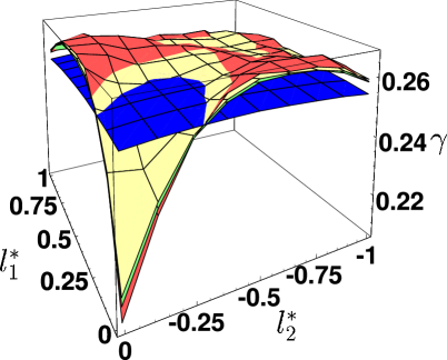
Figure 2: (Color online; monochrome versions have from light to dark: yellow, green, red, blue) The escape rate $\gamma$ (red), as a function of the position of two holes of size $R/20$, together with the first (blue) and second (green) order approximations in Eq. 19 and using one-hole escape rates (yellow) as in Eq. 21. Note that the 3D graphics format does not conceal large fluctuations, for example the RMS deviations from the directly calculated escape rate are 0.00848 (first order), 0.00193 (second order) and 0.00190 (second order using one-hole escape rates).

Figure 3: The escape rate $\gamma$ (solid) as a function of the position of one hole of size $R/50$ at position $l^{*}$, together with the first (dotted) and second (dashed) order approximations in Eq. 19.

Figure 4: As for Fig. 3, except that the hole is of variable size, extending from zero to $l^{*}$.

The results of the numerical simulations for some hole sizes and positions are shown in Figs 2-4. Clearly the second order approximations are better than the first order approximation, especially when both holes are near the same corner, which leads to a lower escape rate. Near a corner, we expect that some orbits have several collisions in the holes, and hence the higher order correlation functions are more important. In Fig. 3 we note that fluctuations in the escape rate as a function of hole position are visible; compare with Ref. [15]. Fig. 4 gives useful information about the validity of the expansion truncated at the first or second term even when the hole is no longer small.

The numerical simulation thus confirm the formulas to second order, which is already sufficient to determine detailed information about the internal dynamics from observing escape rates as a function of hole position. Computation of the necessary higher cumulants where holes are on short periodic orbits will require a deeper analysis of the role of the latter. Another important but only partially understood problem is that of general systems with power law escape, such as stadium-type chaotic billiards, and systems with mixed dynamics, where chaotic and regular behavior coexist. We are confident that our approach (suitably modified) will work and lead to general and useful formulas as well, as suggested by similarities between results in the strongly chaotic systems considered here and in regular systems [19].

L.B. was partially supported by NSF grant DMS-0140165.

References

- [1] \NameMilner V., Hanssen J. L., Campbell W. C. Raizen M. G. \REVIEWPhys. Rev. Lett.8620011514.
- [2] \NameFriedman N., Kaplan A., Carasso D. Davidson N. \REVIEWPhys. Rev. Lett.8620011518.
- [3] \NameSridhar S. \REVIEWPhys. Rev. Lett.671991785.
- [4] \NameJ. Stein H. J. Stockmann \REVIEWPhys. Rev. Lett.6819922867.
- [5] \NameGraf H. D., Harney H. L., Lengeler H., Lewenkopf C. H., Rangacharyulu C., Richter A., Schardt P. Weidenmuller H. A. \REVIEWPhys. Rev. Lett.6919921296.
- [6] \NamePersson E., Rotter I., Stockmann H. J. Barth M. \REVIEWPhys. Rev. Lett.8520002478.
- [7] \NameSweet D., Zeff B. W., Ott E. Lathrop D. P. \REVIEWPhysica D1542001207.
- [8] \NameEllegaard C., Guhr T., Lindemann K., Nygard J. Oxborrow M. \REVIEWPhys. Rev. Lett.7719964918.
- [9] \NameSakamoto T., Takagaki Y., Takaoka S., Gamo K., Murase K. Namba S. \REVIEWJapan J. Appl. Phys.301991L1186.
- [10] \NameBird J. P. \REVIEWJ. Phys. Cond. Mat.111999R413.
- [11] \NameWaalkens H., Burbanks A. Wiggins S. \REVIEWPhys. Rev. Lett.952005084301.
- [12] \NameWaalkens H., Burbanks A. Wiggins S. \REVIEWMon. Not. Roy. Astro. Soc.3612005763.
- [13] \NameTuval I., Schneider J., Piro O. Tel T. \REVIEWEurophys. Lett.652004633.
- [14] \NameMotter A. E. Letelier P. S. \REVIEWPhys. Lett. A2852001127.
- [15] \NameSchneider J., Tel T. Neufeld Z. \REVIEWPhys. Rev. E662002066218.
- [16] \NameBuljan H. Paar V. \REVIEWPhys. Rev. E632001066205.
- [17] \NameMeiss J. D. \REVIEWChaos71997139.
- [18] \NameDemers M. F. Young L.-S. \REVIEWNonlinearity192006377.
- [19] \NameBunimovich L. A. Dettmann C. P. \REVIEWPhys. Rev. Lett.942005100201.
- [20] \NameNagler J., Krieger M., Linke M., Schonke J. Wiersig J. \REVIEWPhys. Rev. E752007046204.
- [21] \NameEvans D. J. Morriss G. P. \BookStatistical mechanics of nonequilibrium liquids \PublAcademic, London\Year1990.
- [22] \NameGaspard P. Nicolis G. \REVIEWPhys. Rev. Lett.6519901693.
- [23] \NameKadanoff L. P. Tang C. \REVIEWProc. Nat. Acad. Sci.8119841276.
- [24] \NameArtuso R., Aurell E. Cvitanović P. \REVIEWNonlinearity31990325.
- [25] \NameDettmann C. P. \REVIEWErgod. Th. Dynam. Sys.232003481.
- [26] \NameChernov N. I. Dettmann C. P. \REVIEWPhysica A297200037
- [27] \NameChernov N. I. Markarian R. \REVIEWCommun. Math. Phys.2702007727
- [28] \NameSantalo L. A. \BookIntegral Geometry and Geometric Probability \PublCUP, Cambridge\Year2004.