Painlevé Analysis and Similarity Reductions for the Magma Equation

Painlevé Analysis and Similarity Reductions
for the Magma Equation

Shirley E. HARRIS ^† and Peter A. CLARKSON ^‡ S.E. Harris and P.A. Clarkson

^† Mathematical Institute, University of Oxford, 24–29 St. Giles’, Oxford, OX1 3LB, UK harris@maths.ox.ac.uk ^‡ Institute of Mathematics, Statistics and Actuarial Science, University of Kent,
  Canterbury, CT2 7NF, UK P.A.Clarkson@kent.ac.uk

Received September 27, 2006; Published online October 05, 2006

In this paper, we examine a generalized magma equation for rational values of two parameters, $m$ and $n$. Firstly, the similarity reductions are found using the Lie group method of infinitesimal transformations. The Painlevé ODE test is then applied to the travelling wave reduction, and the pairs of $m$ and $n$ which pass the test are identified. These particular pairs are further subjected to the ODE test on their other symmetry reductions. Only two cases remain which pass the ODE test for all such symmetry reductions and these are completely integrable. The case when $m=0$, $n=-1$ is related to the Hirota–Satsuma equation and for $m=\tfrac{1}{2}$, $n=-\tfrac{1}{2}$, it is a real, generalized, pumped Maxwell–Bloch equation.

Painlevé analysis; similarity reductions; magma equation

35C05; 35Q58; 37K10

1 Introduction

Scott and Stevenson [26] examine the process of melt migration where buoyant magma rises through the Earth’s mantle. The system is treated as a two-phase flow, with the porous rock matrix able to deform by creep as the melt rises. The model can be written in terms of the porosity or liquid volume fraction $\phi$, i.e. volume of melt in unit volume of the fluid-rock mixture. The constitutive relations $k=k_{0}\phi^{n}$ and $\eta=\eta_{0}\phi^{-m}$ are assumed, where $k$ is the matrix permeability, $\eta$ is an effective viscosity for the matrix and $k_{0}$ and $\eta_{0}$ are constants. After rescaling $\phi$ with its uniform background level, so that the background now corresponds to $\phi=1$, Scott and Stevenson [26] derive the partial differential equation

$$\Delta\equiv\phi_{t}+(\phi^{n}+m\phi^{n-m-1}\phi_{t}\phi_{x}-\phi^{n-m}\phi_{tx})_{x}=0,$$ (1.1)

and suggest that physically appropriate ranges for $m$ and $n$ are

$$0\leq m\leq 1,\qquad 2\leq n\leq 5.$$

The same equation has also been derived independently for $m=0$ by McKenzie [19].

Equation (1.1) is well known to have solitary wave solutions and various authors have examined these. Nakayama and Mason [21] looked for rarefactive solitary waves for which $\phi\geq 1$ everywhere, by using a travelling wave reduction. This leads to

$$c\left({\rm d}\psi\over{\rm d}z\right)^{2}=f(\psi),$$

for some function $f$ where $z=x-ct$ and $\psi(z)=\phi(x,t)$. They then applied the boundary conditions

$$f(1)=0,$$ (1.2a)

$${{\rm d}f\over{\rm d}\psi}(1)=0,$$ (1.2b)

$$f(\Psi)=0,\quad\Psi>1,$$ (1.2c)

and proved that such waves exist if the index $$n>1 0\leq n\leq 1 n\geq 0 (m,n) 0\leq\phi\leq 1$$ and do not exist if , with their analysis restricted to . They go on to derive some solutions for particular values of pairs and to look at the large amplitude approximation. In contrast, in a later paper [23], a perturbation solution for small amplitude rarefactive waves is examined and at leading order has the sech-squared form of a single-soliton solution of the Korteweg–de Vries equation. Nakayama and Mason [20, 22] also look at compressive solitary waves, for which . For boundary conditions, they take the first two to be the same as those for rarefactive waves (1.2a), (1.2b), but in place of the last, they instead use

$${{\rm d}^{2}f\over{\rm d}\psi^{2}}(1)=0.$$ (1.2d)

Zabusky [34] and Jeffrey and Kakutani [15] used this condition for examining algebraic compressive solitary wave solutions of the modified Korteweg–de Vries equation. However, they also found exponential solitary waves and it therefore appears that this choice of boundary condition is limiting. Indeed, in this paper we exhibit some new exponential solitary wave solutions.

In Nakayama and Mason [20], with the boundary conditions (1.2a), (1.2b), (1.2d), the wave speed $c$ must be equal to the index $n$. They derive three compressive solitary wave solutions which tend algebraically to the background $\psi=1$ on either side and reach $\psi=0$ at their maximum amplitude. The wave with $n=m=2$ has a monotone behaviour whereas the one with $n=m=\tfrac{3}{2}$ is oscillatory. The solution for $n=3$ and $m=0$ is not differentiable at the point of maximum amplitude, where there is a cusp. In [22] they examine the necessary conditions for these compressive solitary waves to exist with the same boundary conditions as before. They find that it is necessary to have $n=m>1$ and plot graphs of the curves for integer values $2$, $3$, $4$ and $5$ for $m$ and $n$. It is found that the shape does not greatly change, but that the width increases slowly as $n=m$ increases. The half-integer values $\tfrac{3}{2}$, $\tfrac{5}{2}$, $\tfrac{7}{2}$, and $\tfrac{9}{2}$ are also examined and all prove to have similar oscillatory structure.

Takahashi and Satsuma [29] make a change of variables and find a periodic wave solution for the choice $n=3$, $m=0$ in terms of elliptic integrals. They also investigate weak solutions and demonstrate the possibility of both a hump solution and two travelling wave solutions between different levels with a sharp wavefront. They note that if the if the $\phi_{tx}$ term in (1.1) is replaced by $\phi_{xx}$, it is possible to apply a transformation to yield the Korteweg–de Vries (KdV) equation. However, the transformation is not necessarily single-valued and the significance of this result is unclear. Takahashi, Sachs and Satsuma [28] show that the travelling wave solutions with compact support suggested in [29] are not physically feasible, due to singularities in the stress. They use them, however, as suitable initial conditions for various numerical simulations and demonstrate the break-up into a series of solitary waves.

Marchant and Smyth [18] also examine periodic wave solutions for $n=3$, $m=0$ and develop a modulation theory for slowly varying travelling waves. It is found that full or partial undular bores are possible and there is good comparison between approximate wave envelopes and numerical solutions.

Experiments by Scott, Stevenson and Whitehead [27], Olson and Christensen [24] and Whitehead [31] show solitary waves on conduits of buoyant fluid in a more viscous fluid. The relevant equation is identical to the magma migration equations for $m=1$ and $n=2$ and the experimental results are summarized in Whitehead and Helfrich [33]. They show Korteweg–de Vries ‘soliton-like’ collisions (cf. [10]), in which two solitary waves interact and then emerge unaltered apart from a phase-shift. The experiments also imply that an arbitrary initial condition quickly breaks down into an ordered sequence of solitary waves. These results raise the question about whether the partial differential equation (1.1) is completely integrable (i.e. solvable by the inverse scattering transform) for any of the parameters $m$ and $n$. This is further reinforced by Whitehead and Helfrich  [32] who demonstrate that (1.1) reduces to the KdV equation for small disturbances to the uniform state.

Barcilon and Richter [3] have examined rarefactive waves for $m=0$ and $n=3$ both analytically and numerically. They concluded that this case did not have soliton solutions as there was an interaction left behind by the collision of two solitary waves and they could only find two conservation laws. A completely integrable partial differential equation such as KdV has an infinite number of such laws.

Harris [11] also examines conservation laws for (1.1), without limiting the values of $m$ and $n$ to the physically relevant range, and proved that there were at least three laws for $m=n+1$, $n\neq 0$; at least two laws for $m=1$, $n\neq 0$ and precisely two laws for all other combinations of $m$ and $n$. Thus the special cases $m=n+1$ and $m=1$ (with $n\neq 0$ for both situations) are the only ones which could possibly lead to completely integrable equations.

In this paper, we apply Painlevé analysis to look for any such completely integrable partial differential equations, omitting only the case $m=n=0$ for which the equation is linear. We start by using the Lie group method of infinitesimal transformations to find all the similarity reductions of the partial differential equation to ordinary differential equations. We can then apply the Painlevé ODE test [2] to these and they must all have the Painlevé property (no movable singular points apart from poles) for the partial differential equation to be completely integrable.

Firstly, we examine the travelling wave reduction. Applying the Painlevé ODE test, we find that there are five rational pairs $(m,n)$ which pass for any value of the wave velocity $c$. In addition, there are also four cases which require $c=1$, but these can be discounted as candidates for complete integrability.

The five remaining cases are then subjected to the Painlevé ODE test on their other similarity reductions. Three of these fail the test at this stage, but the other two pass the procedure. These last two cases are then checked with the Painlevé PDE test [30] and are found to be completely integrable.

One case, $m=0$, $n=-1$ is related to the Hirota–Satsuma equation (or Shallow Water Wave I Equation) examined by Clarkson and Mansfield [6]. The second pair, $m=\tfrac{1}{2}$, $n=-\tfrac{1}{2}$, yields a partial differential equation which can be transformed to a special case of the real, generalized, pumped Maxwell–Bloch equation. This has been previously investigated by Clarkson, Mansfield and Milne [7]. We note that both pairs satisfy the criterion of $m=n+1$ given by Harris [11] for the possibility of more than three conservation laws.

2 Symmetry analysis

The classical method for finding symmetry reductions of partial differential equations is the Lie group method of infinitesimal transformations. As this method is entirely algorithmic, though often both tedious and virtually unmanageable manually, symbolic manipulation programs have been developed to aid the calculations. An excellent survey of the different packages available and a description of their strengths and applications is given by Hereman [12, 13]. In this paper we use the MACSYMA package symmgrp.max [5] to calculate the determining equations.

To apply the classical method to equation (1.1), we consider the one-parameter Lie group of infinitesimal transformations in ($x,t,\phi$) given by

$$x^{*}=x+\varepsilon\xi(x,t,\phi)+\mathcal{O}(\varepsilon^{2}),$$

$$t^{*}=t+\varepsilon\tau(x,t,\phi)+\mathcal{O}(\varepsilon^{2}),$$ (2.1)

$$\phi^{*}=\phi+\varepsilon\eta(x,t,\phi)+\mathcal{O}(\varepsilon^{2}),$$

where $\varepsilon$ is the group parameter. Then one requires that this transformation leaves invariant the set

$$S_{\Delta}\equiv\{\phi(x,t):\Delta=0\}$$

of solutions of (1.1). This yields an overdetermined, linear system of equations for the infinitesimals $\xi(x,t,\phi)$, $\tau(x,t,\phi)$ and $\eta(x,t,\phi)$. The associated Lie algebra is realised by vector fields of the form

$$\mathbf{v}=\xi(x,t,\phi){\partial\over\partial x}+\tau(x,t,\phi){\partial\over\partial t}+\eta(x,t,\phi){\partial\over\partial\phi}.$$ (2.2)

Having determined the infinitesimals, the symmetry variables are found by solving the characteristic equation

$${{\rm d}x\over\xi(x,t,\phi)}={{\rm d}t\over\tau(x,t,\phi)}={{\rm d}\phi\over\eta(x,t,\phi)},$$

which is equivalent to solving the invariant surface condition

$$\psi\equiv\xi(x,t,\phi)\phi_{x}+\tau(x,t,\phi)\phi_{t}-\eta(x,t,\phi)=0.$$

The set $S_{\Delta}$ is invariant under the transformation (2.1) provided that ${\rm pr}^{(3)}\mathbf{v}(\Delta)|_{\Delta\equiv 0}=0$ where ${\rm pr}^{(3)}\mathbf{v}$ is the third prolongation of the vector field (2.2), which is given explicitly in terms of $\xi$, $\tau$ and $\eta$ (cf. [25]). This procedure yields a system of 28 determining equations, a linear homogeneous system of equations, for the infinitesimals $\xi(x,t,\phi)$, $\tau(x,t,\phi)$ and $\eta(x,t,\phi)$ as given in Table 1; these were calculated using the MACSYMA package symmgrp.max [5].

Table 1: Infinitesimals for the magma equation (1.1).

$m,\ n$	$\xi$	$\tau$	$\eta$
$n\not=m,\ n\not=0$	$\alpha_{1}x+\alpha_{0}$	$-{(n+m-2)\alpha_{1}\over n-m}t+\alpha_{2}$	${2\alpha_{1}\phi\over n-m}$
$n=m\not=0$	$\alpha_{0}$	$(1-m)\alpha_{1}t+\alpha_{2}$	$\alpha_{1}\phi$
$m\not=\tfrac{4}{3},n=0$	$\alpha_{1}x+\alpha_{0}$	$g(t)$	$-\,{2\alpha_{1}\phi/m}$
$m=\tfrac{4}{3},n=0$	$\alpha_{2}^{2}x^{2}+\alpha_{1}x+\alpha_{0}$	$g(t)$	$-\tfrac{3}{2}(2\alpha_{2}x+\alpha_{1})\phi$

3 Painlevé ODE test on travelling waves

In this section, we use the travelling wave ansatz $\phi(x,t)=\psi(z)$, where $z=x-ct$ to reduce equation (1.1) to the ordinary differential equation

$$c\psi^{2}\psi^{\prime\prime\prime}+c(n-3m)\psi\psi^{\prime}\psi^{\prime\prime}-cm(n-m-1)(\psi^{\prime})^{3}+n\psi^{m+1}\psi^{\prime}-c\psi^{m-n+2}\psi^{\prime}=0,$$ (3.1)

where $(\cdot)^{\prime}$ denotes differentiation with respect to $z$. We then apply the Painlevé ODE test as described in [2], but in order to do this, we must rewrite (3.1) in the form

$$\psi^{\prime\prime\prime}=F(z,\psi,\psi^{\prime},\psi^{\prime\prime}),$$

with the function $F$ analytic in $z$ and rational in its other arguments. If necessary, a transformation must be made before applying the test.

3.1 Integer cases

We will first start by restricting our investigation to $m$ and $n$ being integers so that the criteria on $F$ are satisfied automatically. We now follow [2] and substitute the ansatz

$$\psi\sim\alpha(z-z_{0})^{p},\qquad\alpha\neq 0,$$ (3.2)

into (3.1), with $z_{0}$ being an arbitrary constant. This gives

$$c\alpha^{3}p[p(1-m)-1][p(1-m+n)-2](z-z_{0})^{3p-3}$$

$$\qquad{}+np\alpha^{m+2}(z-z_{0})^{p(m+2)-1}-cp\alpha^{m-n+3}(z-z_{0})^{p(m-n+3)-1}=0.$$ (3.3)

It is initially assumed that this is valid in the neighbourhood of a movable singularity and so ${\rm Re}\,(p)<0$. We examine (3.3) for all possible dominant balances and for each case, we substitute

$$\psi\sim\alpha(z-z_{0})^{p}+\beta(z-z_{0})^{p+r},$$ (3.4)

into the simplified equation obtained by retaining only the dominant terms. Keeping just the linear terms in $\beta$ leads to a cubic equation for $r$ and the solutions of this are known as the resonances of the system. If $p$ is not an integer and if the ansatz (3.2) is asymptotic as $z\to z_{0}$, then the leading order behaviour is that of a branch point. Similarly, if the resonances are not integers, this also indicates the presence of a branch point. If either of these situations occur, then the equation is not of Painlevé type and the case can be rejected. The details of this procedure are given in Table 2, listing $p$, $\alpha$ and the resonances (apart from $r=-1$, which always occurs), along with the conditions on $m$ and $n$ for the balance to be dominant.

Table 2: Results of the Painlevé test for ${\rm Re}\,(p)<0$.

$m,\ n$	$p$	$\alpha$	$r$
$m>1,\ m+n>2$	${1\over{1-m}}$	arbitrary	$0,\ {{m-1+n}\over{m-1}}$
$m>1,\ n>1$	${2\over{1-m}}$	$\left[{2c\over{m-1}}\right]^{1/(m-1)}$	$-2,\ {2n\over{m-1}}$
$m>n,\ n<1,\ m+n\neq 2$	${-2\over{m-n}}$	$\left[{2(2-m-n)\over{(m-n)^{2}}}\right]^{1/(m-n)}$	${2\over{m-n}},\ {2(2-n-m)\over{m-n}}$
$m>1,\ n=c=1$	${1\over{1-m}}$	arbitrary	$0,\ {m\over{m-1}}$
$m>2,\ n=c=1$	${2\over{2-m}}$	arbitrary	$0,\ {-2m\over{m-2}}$
$m>1,\ n=1,\ c\neq 1$	${2\over{1-m}}$	$\left[{2c\over(m-1)(1-c)}\right]^{1/(m-1)}$	$-2,\ {2\over{m-1}}$

We now re-examine (3.3) but considering ${\rm Re}\,(p)>0$ so that $\psi$ itself is finite at $z=z_{0}$ but one of its derivatives may have a singularity. The results for the dominant balances and corresponding values of $p$ and $\alpha$ are presented in Table 3.

Table 3: Results of the Painlevé test for ${\rm Re}\,(p)>0$.

$m,\ n$	$p$	$\alpha$	$r$
$m<1,\ m+n<2$	${1\over{1-m}}$	arbitrary	$0,\ {{1-m-n}\over{1-m}}$
$1+n-m>0,\ n\geq 0$	${2\over{1+n-m}}$	arbitrary	$0,\ {2(m+n-1)\over{1+n-m}}$
$m<1,\ n<1,\ n\neq 0$	${2\over{1-m}}$	$\left[{-2c\over{1-m}}\right]^{1/(m-1)}$	$-2,\ {-2n\over{1-m}}$
$m<n,\ n>1,\ m+n\neq 2$	${2\over{n-m}}$	$\left[{2(2-m-n)\over{(m-n)^{2}}}\right]^{1/(m-n)}$	${-2\over{n-m}},\ {2(n+m-2)\over{n-m}}$
$m<0,\ n=0$	${-2\over{m}}$	$\left[{2(2-m)\over{m^{2}}}\right]^{1/m}$	${2\over{m}},\ {2(2-m)\over{m}}$
$m<1,\ n=c=1$	${1\over{1-m}}$	arbitrary	$0,\ {-m\over{1-m}}$
$m<2,\ n=c=1$	${2\over{2-m}}$	arbitrary	$0,\ {-2m\over{m-2}}$
$m<1,\ n=1,\ c\neq 1$	${2\over{1-m}}$	$\left[{2c\over(1-m)(1-c)}\right]^{1/(m-1)}$	$-2,\ {-2\over{1-m}}$

Considering the results in Tables 2 and 3, we find that there are ten possibilities for integer solutions $m$ and $n$ which give rise to dominant balances with only integer values of $p$ and these are listed in Table 4.

Table 4: Integer solutions of the Painlevé test.

$m$	$n$	$p$	$\alpha$	$r$
0	$-2$	$-1$	$\pm\sqrt{2}$	$\phantom{-}1$,	$\phantom{-}4$
		$\phantom{-}1$	arbitrary	$\phantom{-}0$,	$\phantom{-}3$
		$\phantom{-}2$	$-1/2c$	$-2$,	$\phantom{-}4$
0	$-1$	$-2$	6	$\phantom{-}2$,	$\phantom{-}6$
		$\phantom{-}1$	arbitrary	$\phantom{-}0$,	$\phantom{-}2$
		$\phantom{-}2$	$-1/2c$	$-2$,	$\phantom{-}2$
0	$\phantom{-}1$	$\phantom{-}1$	arbitrary	$\phantom{-}0$,	$\phantom{-}0$
		$\phantom{-}2$	$(c-1)/2c,\,c\neq 1$	$-2$,	$-2$
1	$-1$	$-1$	$\pm 1$	$\phantom{-}1$,	$\phantom{-}2$
1	$\phantom{-}0$	$-2$	2	$\phantom{-}2$,	$\phantom{-}2$
1	$\phantom{-}1$	$\phantom{-}2$	arbitrary	$\phantom{-}0$,	$\phantom{-}2$
1	$\phantom{-}2$	$\phantom{-}1$	arbitrary	$\phantom{-}0$,	$\phantom{-}2$
		$\phantom{-}2$	$-1/2$	$-2$,	$\phantom{-}2$
2	$\phantom{-}1$	$-2$	$2c/(1-c),\,c\neq 1$	$-2$,	$\phantom{-}2$
		$-1$	arbitrary	$\phantom{-}0$,	$\phantom{-}2$
2	$\phantom{-}2$	$-2$	$2c$	$-2$,	$\phantom{-}4$
		$-1$	arbitrary	$\phantom{-}0$,	$\phantom{-}3$
		$\phantom{-}2$	arbitrary	$\phantom{-}0$,	$\phantom{-}6$
2	$\phantom{-}3$	$-2$	$2c$	$-2$,	$\phantom{-}6$
		$-1$	arbitrary	$\phantom{-}0$,	$\phantom{-}4$
		$\phantom{-}1$	arbitrary	$\phantom{-}0$,	$\phantom{-}4$

The resonances in these cases are all integers and they correspond to the points in the solution expansion at which arbitrary constants can be introduced. The resonance $r=-1$ arises from the arbitrariness of $z_{0}$, whilst if $\alpha$ is undetermined, then $r=0$ is another resonance. For each pair ($p$, $\alpha$), we carry out the solution expansion on the full equation in integral powers of $z-z_{0}$, from $(z-z_{0})^{p}$ up as far as $(z-z_{0})^{p+r_{\max}}$, where $r_{\max}$ is the largest positive resonance. If an inconsistency arises, this suggests that logarithmic terms are required in the expansion and hence the ordinary differential equation fails the Painlevé test. A repeated resonance indicates a logarithmic branch point with arbitrary coefficient and this also fails the test [2]. Negative resonances are not well-understood and if they occur for $p<0$, then formally the ordinary differential equation fails the test. In a number of the cases, $r=-2$ occurs in conjunction with $p=2$, but this then corresponds to a Taylor series beginning with a constant term i.e. $p=0$, which was not considered and for which there are no inconsistencies in the expansion. Thus, these particular negative resonances are spurious and can be ignored.

There are four integer cases which pass the test, namely $m=0$, $n=-1$; $m=0$, $n=-2$; $m=n=c=1$ and $m=2$, $n=c=1$. However, the last two only pass for one specific value of the wave speed $c$ and therefore will not be completely integrable.

3.2 Rational cases

When $m$ and $n$ are not integers, we must first transform the third order differential equation (3.1) so that it is in the correct form for applying the Painlevé ODE test. Using the transformation

$$\psi=w^{l},$$ (3.5)

where $l$ is an appropriately chosen positive integer, we can obtain a suitable ordinary differential equation for $w$, where $w^{\prime\prime\prime}$ is a rational function of $w$, $w^{\prime}$ and $w^{\prime\prime}$. We note that if $\psi$ is given by (3.4), then the above transformation gives the equivalent expansion for $w$ as

$$w\sim\alpha_{1}(z-z_{0})^{p_{1}}+\beta_{1}(z-z_{0})^{p_{1}+r_{1}},$$

where

$$p_{1}={p/l},\qquad r_{1}=r.$$ (3.6)

Thus the resonances are left unaltered by this procedure, but the power $p$ is changed by a factor of $l$. We can now use the dominant balances and resonances found for the integer values in Tables 2 and 3, bearing in mind (3.6).

We also note that there are no balances in the list which are appropriate for $m+n=2$, with $m\geq\tfrac{3}{2}$. This suggests that a simple power is not the correct choice of ansatz and that we need to incorporate logarithmic terms at leading order. In fact, we have

$$\psi\sim\alpha(z-z_{0})^{1/(1-m)}[{\rm ln}(z-z_{0})]^{1/(2(1-m))},$$

with

$$\alpha^{2(m-1)}={1\over 2(1-m)}.$$

Thus this case fails the Painlevé test due to the logarithms.

It is now helpful to draw an $mn$-plot to find which regions of the plane will fail the Painlevé test. For negative values of $p$, failure occurs where we have negative resonances and these occur when

$$m>1,\qquad n>1,$$

$$n<1,\qquad m+n>2,$$

$$m>2,\qquad n=1.$$

For positive $p$, we can eliminate the cases where $p+r<0$, namely

$$n\geq 0,\qquad m+n<0,$$

$$m<n,\qquad n>1,\qquad m+n<1,$$

$$m<0,\qquad n=0,$$

$$m<-1,\qquad n=1.$$

We note that if $p/l$ is to be an integer, then $p$ must be an integer and we can use this to rule out further regions in the $mn$-plane. Thus we have failure when $-1<p<0$, which leads to

$$m-n>2,\qquad n<1,\qquad m+n\neq 2.$$

Similarly for positive values of $p$, we have failure if $0<p<1$, and this gives us the two extra conditions

$$m<0, \qquad m+n<2,$$

$$m-n<-1, \qquad n\geq 0.$$

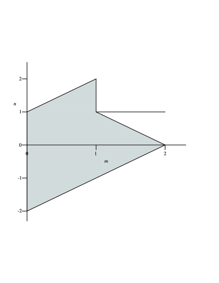
Figure 1: The region of the $mn$-plane which needs to be considered for rational values of $m$ and $n$.

The remaining region is shown in Fig. 1 and includes the boundaries, the shaded interior and the line segment $n=1$, $1\leq m\leq 2$. This can then be examined in more detail to find the rational points which pass the Painlevé test. Those which were not examined in the previous subsection are found to be

$$m={\tfrac{1}{2}},\qquad n=-{\tfrac{1}{2}},$$

$$m={\tfrac{1}{2}},\qquad n=0,$$

$$m={\tfrac{2}{3}},\qquad n=0,$$

$$m={\tfrac{3}{2}},\qquad n=1=c,$$

$$m={\tfrac{4}{3}},\qquad n=1=c.$$

Again, the last two can be discounted as potential candidates for being completely integrable because they only hold for one value of the wave speed $c$.

3.3 Solitary wave solutions

In looking for solitary wave solutions of the magma equations, it is helpful to integrate equation (3.1) twice to yield

$$c(\psi^{\prime})^{2}=-{2\,\psi^{1+m}\over{1-m}}+{2c\,\psi^{2+m-n}\over{2-m-n}}+{2A\,\psi^{1+m-n}\over{1-m-n}}+2B\,\psi^{2m},$$ (3.7)

for $m\neq 1$, $m+n\neq 2$ and $m+n\neq 1$, where $A$ and $B$ are arbitrary constants. Because the scaling on equation (1.1) gave a background level of $\psi=1$, we restrict our interest to this situation.

Nakayama and Mason [21] examined the existence of rarefactive solitary waves for which $\psi\geq 1$ and proved that such waves exist for $n>1$ but do not exist if $0\leq n\leq 1$. Their proof can easily be extended to show that there are no such rarefactive solitary wave solutions for $n<0$. Nakayama and Mason [22] also looked at the existence of compressive solitary waves when $0\leq\psi\leq 1$ and showed that these were only possible when $m=n>1$. However, their boundary conditions were unnecessarily strict, permitting algebraic waves but excluding exponential waves.

Here, we give some exact solutions which are possible when the right hand side of (3.7) is a quartic in $\psi$.

(i)

$m=0$, $n=-2$.

$$\psi=1+{3\sqrt{2}(c+2)\over{\sqrt{27-(c+5)^{2}}\,\cosh\left[\sqrt{{c+2}\over c}(z-z_{0})\right]-\sqrt{2}(1+2c)}}.$$

This solution describes new exponential compressive waves which exist for $-8\leq c<-2$.

(ii)

$m=0$, $n=-1$.

$$\psi=1-{3(c+1)\over{c\cosh\left[\sqrt{{1+c}\over{c}}(z-z_{0})\right]+c}}.$$

This is also a new compressive solitary wave solution when $-3\leq c<-1$ and this is illustrated in Fig. 2 with $c=-2$.

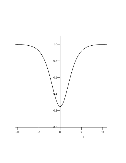
Figure 2: A compressive solitary wave for $m=0$, $n=-1$ when $c=-2$.

(iii)

$m=2$, $n=2$.

$$\psi=1-{{3(c-2)}\over{\pm(1-c)\cosh\left[\sqrt{{c-2}\over c}(z-z_{0})\right]+2c-5}},$$ (3.8a)

$$\psi=1-{12\over{12+(z-z_{0})^{2}}}.$$ (3.8b)

Equation (3.8a) with the positive sign gives a rarefactive solitary wave which exists for $2<c<4$ and agrees with that found by Nakayama and Mason [21]. However, with the minus sign, it represents a new exponential compressive wave solution of amplitude 1 for $c<0$ and $c>2$ and on letting $c\to 2$, it gives the algebraic wave (3.8b) seen in Nakayama and Mason [20]. These waves are shown in Fig. 3, for different values of the wave speed $c$.

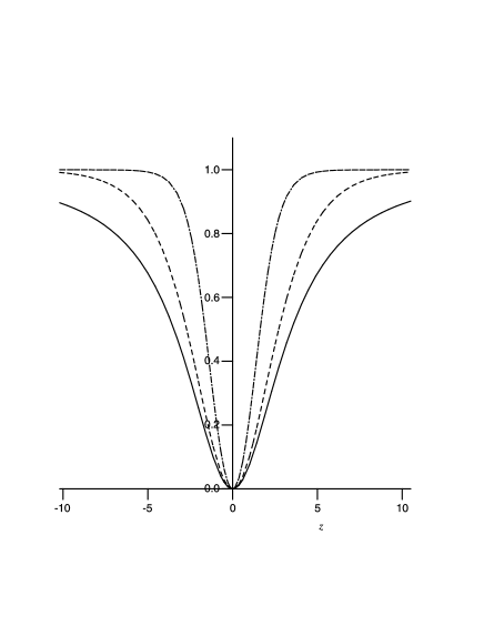
Figure 3: Solitary waves for $m=2$, $n=2$, which are exponential for $c=-2$ ($-\cdot-$) and $c=3$ ($-\,-\,-$) and algebraic when $c=2$ (——).

We now look at other rational values of $m$ and $n$. By using the substitution (3.5) to transform equation (3.7) into an equation for $w$ of the form

$$\left(w^{\prime}\right)^{2}=f(w),$$

and looking for values of $m$ and $n$ which give $f(w)$ as a quartic polynomial, we can find further solutions of this form. It turns out that only $l=2$ is possible for real solutions, and the equation for $w$ is

$$\left(w^{\prime}\right)^{2}=-{w^{2m}\over{2c(1-m)}}+{w^{2+2m-2n}\over{2(2-m-n)}}+{Aw^{2m-2n}\over{2c(1-m-n)}}+{B\over{2c}}w^{4m-2}.$$

The values of $m$ for which both the first and last terms on the right hand side can give a quartic in $w$ are $m=\tfrac{1}{2}$ and $m=\tfrac{3}{2}$ (with $m=1$ being excluded as the denominator of the first term would vanish). Choosing appropriate values for $A$ and $B$ so that there is a double root of the right hand side at $w=1$, we can find solutions for $w$ and hence $\psi$.

(iv)

$m=\tfrac{1}{2}$, $n=-\tfrac{1}{2}$, with $c<-\tfrac{1}{2}$.

$$\psi=\left(1+{{1+2c}\over{\sqrt{-\tfrac{1}{2}c}\,\cosh\left[{\sqrt{{1+2c}\over{2c}}(z-z_{0})}\right]-c}}\right)^{2}$$

This is a compressive wave which is oscillatory for $c<-2$ and represents a new solution. (See Fig. 4.)

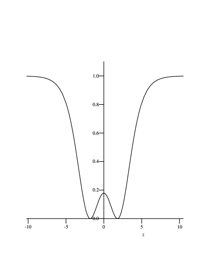
Figure 4: An oscillatory solitary wave for $m=-{1\over 2}$, $n=-{1\over 2}$ when $c=-6$.

(v)

$m=\tfrac{1}{2}$, $n=0$.

$$\psi=\left(1-{6\over{\cosh(z-z_{0})+1}}\right)^{2}.$$

This new solution is oscillatory in nature, has both compressive and rarefactive regions and the shape is independent of velocity. (See Fig. 5.)

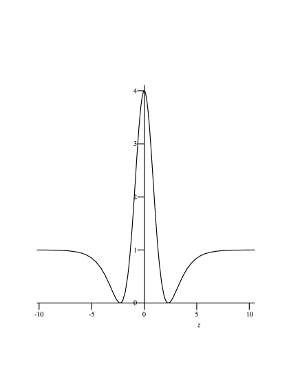
Figure 5: A solitary wave with compressive and rarefactive regions for $m={1\over 2}$, $n=0$.

(vi)

$m=\tfrac{3}{2}$, $n=1$.

$$\psi=\left(1-{6\over{\cosh\left[{\sqrt{{c-1}\over c}(z-z_{0})}\right]+5}}\right)^{2}.$$

This is a compressive wave with amplitude 1 for $c<0$ or $c>1$.

(vii)

$m=\tfrac{3}{2}$, $n=\tfrac{3}{2}$.

$$\psi=\left(1+{{2c-3}\over{\pm\sqrt{{c-1}\over 2}\cosh\left[{\sqrt{{2c-3}\over 2c}(z-z_{0})}\right]+2-c}}\right)^{2},$$ (3.9a)

$$\psi=\left(1-{12\over{(z-z_{0})^{2}+9}}\right)^{2}.$$ (3.9b)

Equation (3.9a) represents rarefactive waves with the positive root if $3>c>\tfrac{3}{2}$ (found by Nakayama and Mason [21] whereas it gives new compressive oscillatory waves for $c>\tfrac{3}{2}$ for the negative root. As $c\to\tfrac{3}{2}$ for the compressive wave, we find the algebraic solution (3.9b) which is given in Nakayama and Mason [20].

4 Other scaling reductions

For the five cases which pass the Painlevé ODE test on the travelling wave reduction, we now look at the test on the other symmetry reductions found in Section 2.

(i)

$m=0$, $n=-2$. Using the reduction,

$$z=xt^{{1/2}},\qquad\phi(x,t)=t^{{1/2}}w(z)$$

leads to the equation

$$zww^{\prime\prime\prime}-2zw^{\prime}w^{\prime\prime}-zw^{3}w^{\prime}+3ww^{\prime\prime}-4(w^{\prime})^{2}+4w^{\prime}-w^{4}=0.$$ (4.1)

(ii)

$m=0$, $n=-1$. Here the appropriate reduction is

$$z=xt^{{1/3}},\qquad\phi(x,t)=t^{{2/3}}w(z),$$

leading to the equation

$$zww^{\prime\prime\prime}-zw^{\prime}w^{\prime\prime}-zw^{2}w^{\prime}+4ww^{\prime\prime}-3(w^{\prime})^{2}+3w^{\prime}-2w^{3}=0.$$ (4.2)

(iii)

$m=\tfrac{1}{2}$, $n=-\tfrac{1}{2}$. In this case, we use

$$z=xt^{{1/2}},\qquad\phi(x,t)=tw^{2}(z)$$

to obtain

$$zww^{\prime\prime\prime}-zw^{\prime}w^{\prime\prime}-zw^{3}w^{\prime}+3ww^{\prime\prime}-2(w^{\prime})^{2}+w^{\prime}-w^{4}=0.$$ (4.3)

(iv)

$m=\tfrac{1}{2}$, $n=0$. The correct reduction for this case is

$$z=xh(t),\qquad\phi(x,t)=x^{-4}w^{2}(z)$$

where $h$ is an arbitrary function and this leads to the equation

$$z^{2}w^{\prime\prime\prime}-2zw^{\prime\prime}-ww^{\prime}+2w^{\prime}=0.$$ (4.4)

(v)

$m=\tfrac{2}{3}$, $n=0$. Lastly, we have the reduction

$$z=xh(t),\qquad\phi(x,t)=x^{-3}w^{3}(z)$$

yielding

$$z^{2}w^{\prime\prime\prime}-w^{2}w^{\prime}=0.$$ (4.5)

As in the travelling wave reductions, we again use the ansatz

$$\psi\sim\alpha(z-z_{0})^{p},\qquad\alpha\neq 0,$$

to find the dominant balances for ${\rm Re}\,(p)<0$ and the resulting resonances, with $r=-1$ always occurring due to the arbitrariness of $z_{0}$. The results are shown in Table 5 and give integer values for $p$ and $r$.

Table 5: Results of the Painlevé test for ${\rm Re}\,(p)<0$.

$m$	$n$	$p$	$\alpha$	$r$
0	$-2$	$-1$	$\pm\sqrt{2}$	$1$,	$4$
0	$-1$	$-2$	$6$	$2$,	$6$
${1\over 2}$	$-{1\over 2}$	$-1$	$\pm 2$	$2$,	$4$
${1\over 2}$	$0$	$-2$	$12\,z_{0}^{2}$	$4$,	$6$
${2\over 3}$	$0$	$-1$	$\pm\sqrt{6}\,z_{0}$	$3$,	$4$

However, for cases (4.1), (4.4) and (4.5), the solution expansion on the full equation as far as powers of $(z-z_{0})^{p+r_{\max}}$ gives inconsistencies, indicating that logarithmic terms are required in the expansion. Therefore, these cases fail the Painlevé test. This leads to only cases (4.2) and (4.3) remaining, which both satisfy the condition $m=n+1$ found by Harris [11].

5 Painlevé PDE test

In this section, we consider the two remaining cases and relate them to known completely integrable equations.

(i)

$m=0$, $n=-1$. A slightly more general equation is considered, namely

$$\phi\phi_{xxt}-\phi_{x}\phi_{xt}-\phi^{2}\phi_{t}+\mu\phi_{x}=0,$$ (5.1)

which reduces to the magma equation for $m=0$, $n=-1$ upon setting $\mu=1$.

It is straightforward to apply the Painlevé PDE test, as described by Weiss, Tabor and Carnevale [30], to (5.1) and it is found to pass the test for any values of $\mu$. We note that (5.1) can be written in the form

$$\left[\left(\phi_{xt}-\mu\right)/\phi\right]_{x}-\phi_{t}=0.$$

Then making the transformation $\phi=v_{x}$ and integrating once gives

$$v_{xxt}-v_{x}v_{t}-\mu=0,$$

where we have set the function of integration to zero, without loss of generality. A simple transformation

$$v(x,t)=-u(x,t)-x-t$$

then leads to the shallow water wave (SWWI) equation

$$u_{xxxt}+u_{x}u_{xt}+u_{t}u_{xx}-u_{xt}-u_{xx}=0,$$ (5.2)

which was considered by Clarkson and Mansfield [6]. This is also equivalent to the Hirota–Satsuma equation

$$\eta_{xxt}+\eta\eta_{t}-\eta_{x}\partial_{x}^{-1}(\eta_{t})-\eta_{x}-\eta_{t}=0,$$ (5.3)

where $\partial^{-1}_{x}(f)(x)=\int_{x}^{\infty}f(y)\,{\rm d}y$, which was discussed by Hirota and Satsuma [14].

Clarkson and Mansfield [6] have discussed symmetry reductions of (5.2) obtainable using the classical Lie method and the nonclassical method of [4]. They gave a catalogue of classical and nonclassical symmetry reductions and exact solutions of (5.2). Of particular interest are a plethora of solutions of (5.2) possessing a rich variety of qualitative behaviours. These arise as nonclassical symmetry reductions and all of which look like a two-soliton solution as $t\to-\infty$, yet are radically different as $t\to\infty$. These results have important implications with regard to numerical analysis and suggest that solving (5.2) numerically could pose some fundamental difficulties. An exponentially small change in the initial data yields a fundamentally different solution as $t\to\infty$. How can any numerical scheme in current use cope with such behaviour? (See [6] for further details.)

The Lax pair for the Hirota–Satsuma equation (5.3) is the third scattering order problem [8]

$$\psi_{xxx}-\left(1+\tfrac{1}{2}\eta\right)\psi_{x}=\lambda\psi,$$ (5.4a)

$$3\lambda\psi_{t}=[1-\partial^{-1}_{x}(\eta_{t})]\psi_{xx}-\eta_{t}\psi_{x}.$$ (5.4b)

We remark that (5.4a) is similar to the scattering problem

$$\psi_{xxx}+\tfrac{1}{4}(1+6u)\psi_{x}+\tfrac{3}{4}\left[u_{x}-{\rm i}\sqrt{3}\,\partial_{x}^{-1}(u_{t})\right]\psi=\lambda\psi,$$

which is the scattering problem for the Boussinesq equation

$$u_{xxxx}+3(u^{2})_{xx}+u_{xx}=u_{tt},$$

and has been comprehensively studied by Deift, Tomei and Trubowitz [9].

(ii)

$m=\tfrac{1}{2}$, $n=-\tfrac{1}{2}$. Similarly, we consider a slightly more general equation

$$uu_{xxt}-u_{x}u_{xt}-u^{3}u_{t}+\mu u_{x}=0,$$ (5.5)

where setting $\phi(x,t)=u^{2}$ and $\mu=\tfrac{1}{2}$ yields the magma equation for $m=\tfrac{1}{2}$, $n=-\tfrac{1}{2}$.

Again, the Painlevé PDE test due to Weiss, Tabor and Carnevale [30] can be applied and (5.5) is found to pass for any $\mu$. Clarkson, Mansfield and Milne [7] showed that (5.5) arises as a symmetry reduction of the $(2+1)$-dimensional Sine-Gordon system

$$\left({\Theta_{XT}\over\sin\,\Theta}\right)_{X}-\left({\Theta_{YT}\over\sin\Theta}\right)_{Y}-{\Theta_{Y}R_{XT}-\Theta_{X}R_{YT}\over\sin^{2}\Theta}=0,$$

$$\left({R_{XT}\over\sin\Theta}\right)_{X}-\left({R_{YT}\over\sin\Theta}\right)_{Y}-{\Theta_{Y}\Theta_{XT}-\Theta_{X}\Theta_{YT}\over\sin^{2}\Theta}=0,$$

derived by Konopelchenko and Rogers [16, 17]. The special case of (5.5) with $\mu\equiv 0$ is equivalent to the sine-Gordon equation

$$u_{xt}=\sin u,$$ (5.6)

which is one of the fundamental soliton equations solvable by inverse scattering using the AKNS method [1].

Clarkson, Mansfield and Milne [7] show that a Lax pair associated with (5.5) is given by

$${\boldsymbol{\psi}}_{x}=\left\{-{\rm i}\lambda{\boldsymbol{\sigma}}_{3}-\tfrac{1}{2}{\rm i}u{\boldsymbol{\sigma}}_{2}\right\}{\boldsymbol{\psi}},$$ (5.7a)

$${\boldsymbol{\psi}}_{t}=\left\{{\rm i}{u_{xt}-\mu\over 4\lambda u}{\boldsymbol{\sigma}}_{3}+{{\rm i}u_{t}\over 4\lambda}{\boldsymbol{\sigma}}_{1}-{{\rm i}\mu\over 8\lambda^{2}}{\boldsymbol{\sigma}}_{2}\right\}{\boldsymbol{\psi}}=0.$$ (5.7b)

where ${\boldsymbol{\sigma}}_{1}$, ${\boldsymbol{\sigma}}_{2}$ and ${\boldsymbol{\sigma}}_{3}$ are the Pauli spin matrices given by

$${\boldsymbol{\sigma}}_{1}=\left(\begin{array}[]{cr}0&1\\ 1&0\end{array}\right),\qquad{\boldsymbol{\sigma}}_{2}=\left(\begin{array}[]{cr}0&-{\rm i}\\ {\rm i}&0\end{array}\right),\qquad{\boldsymbol{\sigma}}_{3}=\left(\begin{array}[]{cr}1&0\\ 0&-1\end{array}\right).$$

Equations (5.7) are compatible, i.e. ${\boldsymbol{\psi}}_{xt}={\boldsymbol{\psi}}_{tx}$ provided that $u(x,t)$ satisfies (5.5). We remark that the Lax pair (5.7) reduces to that for the sine-Gordon equation (5.6) if $\mu=0$ [1]. Further we note that the spectral problem (5.7a) is the standard AKNS spectral problem whilst if $\mu\not=0$, then (5.7b) involves powers of both $\lambda^{-1}$ and $\lambda^{-2}$.

6 Discussion

We have performed a comprehensive Painlevé analysis of the generalized magma equation

$$\phi_{t}+(\phi^{n}+m\phi^{n-m-1}\phi_{t}\phi_{x}-\phi^{n-m}\phi_{tx})_{x}=0,$$

and found that there are only two pairs of values of the indices $m$ and $n$ for which the equation is completely integrable. The case $m=0$, $n=-1$ is related to the Hirota–Satsuma equation and was studied by Clarkson and Mansfield [6]. The Hirota bilinear form, multi-soliton solutions and the Lax pair are known for this equation. The situation when $m=\tfrac{1}{2}$, $n=-\tfrac{1}{2}$ is less clear cut. It is related by a simple transformation to a special case of the real, generalized, pumped Maxwell–Bloch system examined by Clarkson, Mansfield and Milne [7]. It has an non-isospectral Lax Pair and a single soliton solution, but the Hirota bilinear form and multi-soliton solutions are as yet unknown.

Acknowledgements

It is a pleasure to thank Elizabeth Mansfield and Andrew Pickering for their helpful comments and discussions. SEH gratefully acknowledges the support of a Darby Fellowship at Lincoln College, Oxford and a Grace Chisholm Young Fellowship from the London Mathematical Society for the period in which this research was carried out. PAC thanks the Isaac Newton Institute, Cambridge for their hospitality during his visit as part of the programme on “Painlevé Equations and Monodromy Problems” when this paper was completed.

References

- [1] Ablowitz M.J., Kaup D.J., Newell A.C., Segur H., The inverse scattering transform – Fourier analysis for nonlinear problems, Stud. Appl. Math., 1974, V.53, 249–315.
- [2] Ablowitz M.J., Ramani A., Segur H., A connection between nonlinear evolution equations and ordinary differential equations of P-type. I, J. Math. Phys., 1980, V.21, 715–721.
- [3] Barcilon V., Richter F.M., Nonlinear waves in compacting media, J. Fluid Mech., 1986, V.164, 429–448.
- [4] Bluman G.W., Cole J.D., The general similarity solution of the heat equation, J. Math. Mech., 1969, V.18, 1025–1042.
- [5] Champagne B., Hereman W., Winternitz P., The computer calculation of Lie point symmetries of large systems of differential equations, Comput. Phys. Comm., 1991, V.66, 319–340.
- [6] Clarkson P.A., Mansfield E.L., On a shallow water wave equation, Nonlinearity, 1994, V.7, 975–1000, solv-int/9401003.
- [7] Clarkson P.A., Mansfield E.L., Milne A.E., Symmetries and exact solutions of a -dimensional Sine-Gordon system, Phil. Trans. R. Soc. Lond. A, 1996, V.354, 1807–1835, solv-int/9412003.
- [8] Conte R., Musette M., Grundland A.M., Bäcklund transformation of partial differential equations from the Painlevé-Gambier classification. II. Tzitzeica equation, J. Math. Phys., 1999, V.40, 2092–2106.
- [9] Deift P., Tomei C., Trubowitz E., Inverse scattering and the Boussinesq equation, Commun. Pure Appl. Math., 1982, V.35, 567–628.
- [10] Drazin P.G., Johnson R.S., Solitons: an introduction, Cambridge, Cambridge University Press, 1989.
- [11] Harris S.E., Conservation laws for a nonlinear wave equation, Nonlinearity, 1996, V.9, 187–208.
- [12] Hereman W., Symbolic software for Lie symmetry analysis, in CRC Handbook of Lie Group Analysis of Differential Equations. III. New Trends in Theoretical Developments an Computational Methods, Editor N.H. Ibragimov, Boca Raton, CRC Press, 1996, Chapter XII, 367–413.
- [13] Hereman W., Review of symbolic software for Lie symmetry analysis, Math. Comput. Modelling, 1997, V.25, 115–132.
- [14] Hirota R., Satsuma J., -soliton solutions of model equations for shallow water waves, J. Phys. Soc. Japan, 1976, V.40, 611–612.
- [15] Jeffrey A., Kakutani T., Weak nonlinear dispersive waves: a discussion centered around the Korteweg–de Vries equation, SIAM Rev., 1972, V.14, 582–643.
- [16] Konopelchenko B.G., Rogers C., On -dimensional nonlinear systems of Loewner type, Phys. Lett. A, 1991, V.158, 391–397.
- [17] Konopelchenko B.G., Rogers C., On generalized Loewner systems: novel integrable equations in -dimensional, J. Math. Phys., 1993, V.34, 214–242.
- [18] Marchant T.R., Smyth N.F., Approximate solutions for magmon propagation from a reservoir, IMA J. Appl. Math., 2005, V.70, 796–813.
- [19] McKenzie D.P., The generation and compaction of partially molten rock, J. Petrol., 1984, V.25, 713–765.
- [20] Nakayama M., Mason D.P., Compressive solitary waves in compacting media, Internat. J. Non-Linear Mech., 1991, V.26, 631–640.
- [21] Nakayama M., Mason D.P., Rarefactive solitary waves in two–phase fluid flow of compacting media, Wave Motion, 1992, V.15, 357–392.
- [22] Nakayama M., Mason D.P., On the existence of compressive solitary waves in compacting media, J. Phys. A: Math. Gen., 1994, V.27, 4589–4599.
- [23] Nakayama M., Mason D.P., Perturbation solution for small amplitude solitary waves in two-phase fluid flow of compacting media, J. Phys. A: Math. Gen., 1999, V.32, 6309–6320.
- [24] Olson P., Christensen U., Solitary wave propagation in a fluid conduit within a viscous matrix, J. Geophys. Res., 1986, V.91, 6367–6374.
- [25] Olver P.J., Applications of Lie groups to differential equations, 2nd ed., Graduate Texts Math., Vol. 107, New York, Springer, 1993.
- [26] Scott D.R., Stevenson D.J., Magma solitons, Geophys. Res. Lett., 1984, V.11, 1161–1164.
- [27] Scott D.R., Stevenson D.J., Whitehead J.A., Observations of solitary waves in a viscously deformable pipe, Nature, 1986, V.319, 759–761.
- [28] Takahashi D., Sachs J.R., Satsuma J., Properties of the magma and modified magma equations, J. Phys. Soc. Japan, 1990, V.59, 1941–1953.
- [29] Takahashi D., Satsuma J., Explicit solutions of magma equation, J. Phys. Soc. Japan, 1988, V.57, 417–421.
- [30] Weiss J., Tabor M., Carnevale G., The Painlevé property for partial differential equations, J. Math. Phys., 1983, V.24, 522–526.
- [31] Whitehead J.A., A laboratory demonstration of solitons using a vertical watery conduit in syrup, Amer. J. Phys., 1987, V.55, 998–1003.
- [32] Whitehead J.A., Helfrich K.R., The Korteweg–de Vries equation from conduit and magma migration equations, Geophys. Res. Lett., 1986, V.13, 545–546.
- [33] Whitehead J.A., Helfrich K.R., Magma waves and diapiric dynamics, in Magma Transport and Storage, Editor M.P. Ryan, Wiley & Sons, 1990, 53–76.
- [34] Zabusky N.J., A synergetic approach to problems of nonlinear dispersive wave propagation and interaction, in Proc. Symp. Nonlinear Partial Differential Equations, Editor W. Ames, New York, Academic Press, 1967, 223–258.