Coalescing Cellular Automata

Abstract

We say that a Cellular Automata (CA) is coalescing when its execution on two distinct (random) initial configurations in the same asynchronous mode (the same cells are updated in each configuration at each time step) makes both configurations become identical after a reasonable time. We prove coalescence for two elementary rules and show that there exists infinitely many coalescing CA. We then conduct an experimental study on all elementary CA and show that some rules exhibit a phase transition, which belongs to the universality class of directed percolation.

1 Introduction

The coalescence phenomenon, as we call it, has been observed for the first time by Nazim Fates [1], in the context of asynchronous cellular automata. Coalescing CA exhibit the following behavior: starting from two different initial random configurations and running the same updating sequence (the same cells are updated at each time step in both configurations), the configurations quickly become identical, i.e. the dynamics not only reach the same attractor, they also synchronize their orbits. This of course appears in trivial situations, for example if the CA converges on a single fixed point, but Nazim Fates has also observed it in a case where the coalescing orbit is absolutely non trivial.

The goal of this paper is to explore this rather strange emergent phenomenon in which the asymptotic behavior seems to be only related to the (random) sequence of update of the cells and not to the initial configuration. This work shows that, in some cases, the randomness used during evolution is as important as the one used during initialization: this stochastic dynamic, with high entropy, is perfectly insensitive to initial condition (no chaos here).

The results presented here are of two kinds. First, we prove the existence of infinitely many different (we precise this notion) non trivial coalescent CA. Secondly, we study by simulation the behavior of all elementary CA (ECA) with regards of this coalescence property, in an asynchronous context in which at each step each cell has a fixed probability $\alpha$ to be updated. We show that over the 88 different ECA, six situations occur: a/ 37 ECA never coalesce; b/ 20 always coalesce in a trivial way (they converge to a unique fixed point); c/ 6 always coalesce on non trivial orbits; d/ 14 combine a/, b/ and c/ depending on $\alpha$ (4 combine a/ and b/, 3 combine b/ and c/, and 7 combine a/ and c/); e/ 7 enter either full agreement (coalescence) or full disagreement; last, f/ 4 combine e/ with either a/, b/ or c/.

We also study the transition between non coalescence and coalescence when $\alpha$ varies for the ECA that combine a/ and c/: there is a phase transition belonging to the universality class of directed percolation. We thus get a new model of this class, with a few variants. An unusual fact among directed percolation models is that the limit of the sub-critical regime is neither a single absorbing state, nor a set of fixed points, but a non trivially evolving phase. Its originality and links to other domains could help understanding this class and hopefully lead to analytical results.

The paper is organized as follows. Section 2 gives definitions and notations. We prove in section 3 that, under certain conditions, CA $\mathfrak{6}$ and $\mathfrak{7}$ (using the Wolfram’s numbering of ECA) are coalescing and show how to construct from them coalescing CA with arbitrarily many states. We also prove that CA $\mathfrak{15}$ and $\mathfrak{170}$ either coalesce or enter total disagreement, each case occurring with probability $\frac{1}{2}$. In Section 4, we describe the exhaustive simulation study of all ECA and then check the directed percolation hypothesis. Moreover, we prove that some CA exhibit two phase transitions: one for small $\alpha$ and one for high $\alpha$.

2 Definitions and Notations

In this paper, we consider the dynamics of some CA when they are run on an asynchronous mode. Let us start by defining the synchronisms we work with.

Definition 1

An asynchronous finite CA is a tuple $(Q,\,d,\,V,\,\delta,\,n,\,\mu)$ where

• $Q$ is the set of states;

• $d\in\mathbb{N}^{*}$ is the dimension;

• $V=\{v_{1},\,\dots,\,v_{|V|}\}$, the neighborhood, is a finite set of vectors in $\mathbb{Z}^{d}$;

• $\delta:Q^{|V|}\to Q$ is the transition rule;

• $n\in\mathbb{N}^{*}$ is the size;

• ${\cal U}:=(\mathbb{Z}/n\mathbb{Z})^{d}$ is the cell space (with periodic boundary condition);

• $\mu$, the synchronism, is a probability measure on $\{0,1\}^{\cal U}$.

A configuration specifies the state of each cell, and so is a function $c:{\cal U}\to Q$.

The dynamic is then the following. Let $c_{t}$ denote the configuration at time $t$, ($c_{0}$ is the initial configuration). Let $\left\{M_{t}\ \left|\ \vphantom{M_{t}}t\in\mathbb{N}\right.\right\}$ be a sequence of independent identically distributed random variables with distribution $\mu$. The configuration at time $t+1$ is obtained by

$$c_{t+1}(z):=\begin{cases}c_{t}(z)&\text{if }M_{t}(z)=0\\ \delta\big{(}c_{t}(z+v_{1}),\,\dots,\,c_{t}(z+v_{|V|})\big{)}&\text{if }M_{t}(z)=1\\ \end{cases}\ .$$

In other words, for each cell $z$, we apply the usual transition rule if $M_{t}(z)=1$ and freeze it (keep its state) if $M_{t}(z)=0$.

Here are the two synchronisms we use. They are the most natural, even if others are possible (like systematic or alternating sweep, or updating some cells more often, but this require non independent $M_{t}$ and so a more general formalism). If $x\in\{0,1\}^{\cal U}$, let $|x|_{1}$ be the number of 1 in the coordinates of $x$.

The Partially Asynchronous Dynamic Let $0<\alpha\leq 1$. For each cell, we update it with probability $\alpha$, independently from its neighbors. $\mu$ is thus the product measure of Bernoulli distributions: $\mu(x):=\alpha^{|x|_{1}}(1-\alpha)^{|x|_{0}}$ (with $0^{0}=1$). The case $\alpha=1$ corresponds to the synchronous dynamic.

The Fully Asynchronous Dynamic At each step, we choose one cell and update it. Which defines $\mu(x)$ as $1/n$ if $|x|_{1}=1$ and $\mu(x):=0$ otherwise.

We now introduce the definition of coalescing CA to formalize the observation of [1]. The principle is to use two initial configurations, and to let them evolve with the same outcome of the random variables $\left\{M_{t}\ \left|\ \vphantom{M_{t}}t\in\mathbb{N}\right.\right\}$. In other words, we use two copies of the CA, and at each time step, we update the same cells in both copies. This comes down to using the same source of randomness for both copies, like in [2] (on another system) where the authors observe a synchronization.

Definition 2

An asynchronous finite CA is coalescing if, for any two initial configurations, applying the same sequence of updates leads both configurations to become identical within polynomial expected time (with respect to $n$).

Any nilpotent CA (converging toward a configuration where all states are identical) is coalescing if it converges in polynomial time. But there are non nilpotent coalescing CA, which we call non trivial. We now consider only those CA.

In the following, we heavily use the simplest CA, namely the Elementary CA: one dimension ($d=1$), $2$ states ($Q=\{0,1\}$), nearest neighbors ($V=\{-1,0,1\}$). There are $2^{8}=256$ possible rules, $88$ after symmetry considerations. We use the notation introduced by S. Wolfram, numbering the rules from $\mathfrak{0}$ to $\mathfrak{255}$.

3 Formal Proof of Coalescence

In this section, we prove that there are infinitely many coalescing CA. For that, we prove the coalescence of two particular CA and show how to build an infinite number of coalescing CA from one of them. An easy way to do that last point would be to extend a coalescing CA by adding states that are always mapped to one states of the original CA, regardless of their neighbors. However, we consider such a transformation to be artificial since it leads to a CA that is in some sense identical. To avoid this, we focus on state minimal CA: CA in which any state can be reached. Note that among ECA, only $\mathfrak{0}$ and $\mathfrak{255}$ are not state-minimal.

We first exhibit two state-minimal coalescing CA (proposition 1); then, using this result, deduce the existence of an infinite number of such CA (theorem 3.1); and finally describe the coalescent behavior of two others ECA (proposition 2).

Proposition 1

Rules $\mathfrak{6}$ and $\mathfrak{7}$ are coalescing for the fully asynchronous dynamic when $n$ is odd.

Proof

We call number of zones the number of patterns $01$ in a configuration, which is the number of “blocks” of consecutive $1$ (those blocks are the zones). We first consider only one copy (one configuration).

[r] Neighbors 1 1 1 1 1 0 1 0 1 1 0 0 0 1 1 0 1 0 0 0 1 0 0 0 New state 0 0 0 0 0 1 1 0 Here is the transition table of $\mathfrak{6}$. Since one cell at a time is updated, and updating the central cell of $101$ or $010$ does not change its state, zones cannot merge.

[r]$\begin{matrix}\cdots\ 0\ \underbrace{0\ 0\ 1}\ \cdots\\ \cdots\ \underbrace{0\ 0\ 1}\ 1\ \cdots\\ \cdots\ 0\ \underbrace{1\ 1\ 1}\ \cdots\\ \cdots\ 0\ 1\ 0\ 1\ \cdots\end{matrix}$ On each pattern $111$, the central cell can be updated (leading to the pattern $101$) before its neighbors (with probability $\frac{1}{3}$) with expected time $n$. On each pattern $0001$, the opposite sequence is possible. It happens without other update of the four cells with probability $1/4^{3}$ and with an expected time of $3\,n$. So, as long as there are patterns $000$ or $111$, the number of zones increases with an expected time $O(n)$. Since there are $O(n)$ zones, the total expected time of this increasing phase is $O(n^{2})$.

The configuration is then regarded as a concatenation of words on $\{0,\,1\}^{*}$. Separation between words are chosen to be the middle of each pattern $00$ and $11$, so we get a sequence of words that have no consecutive identical letters, each word being at least two letter long (that is, words of the language “$(01)^{+}0?\ |\ (10)^{+}1?$”). We now show that borders between these words follow a one way random walk (towards right) and meet, in which case a word disappear with positive probability. The CA evolves therefore towards a configuration with only one word.

Updating the central cell of $100$ does not change its state, so the borders cannot move towards left more than one cell. On the other hand, updating the central cell of $001$ or $110$ make the border move. One step of this random walk takes an expected time $O(n)$.

The length of a word also follows a (non-biased) random walk, which reaches $1$ after (on average) $O(n^{3})$ steps, leading to the pattern $000$ or $111$. This pattern disappears with a constant non zero probability like in the increasing phase. The expected time for $O(n)$ words to disappear is then $O(n^{4})$.

Since $n$ is odd, the two letters at the ends of the words are the same, i.e. there is one single pattern $00$ or $11$, still following the biased random walk. We now consider again the two copies. This pattern changes the phase in the sequence $(01)^{+}$, it is therefore a frontier between a region where both configurations agree and a region where they do not. The pattern in the other configuration let us come back to the region where the configurations have coalesced. We study the length of the (single) region of disagreement. It follows a non biased random walk determined by the moves of both patterns.

[r]$\begin{matrix}\cdots\ 1\ 0\ 1\ 0\ 0\ 1\ 0\ 1\ \cdots\\[-2.15277pt] \cdots\ 0\ 1\ 0\ 1\ 1\ 0\ 1\ 0\ \cdots\end{matrix}$ When this length reaches $n$, as opposite, the only change happens when the fourth cell is updated, and it decreases the length. So, the random walk cannot indefinitely stay in state $n$.

[r]$\begin{matrix}\cdots\ 0\ 1\ 0\ 1\ 0\ 0\ 1\ 0\ \cdots\\[-2.15277pt] \cdots\ 0\ 1\ 0\ 1\ 1\ 0\ 1\ 0\ \cdots\end{matrix}$ On the other hand, when the length reaches $1$, one possibility is the opposite, where updating the fifth cell leads to coalescence.

[r]$\begin{matrix}\cdots\ 0\ 1\ 0\ 1\ 1\ 0\ 1\ 0\ \cdots\\[-2.15277pt] \cdots\ 0\ 1\ 0\ 0\ 1\ 0\ 1\ 0\ \cdots\end{matrix}$ The other possibility is opposite, where updating the fifth then the fourth cell leads to the former possibility. In each case, coalescence happens with a constant non zero probability. One step of this random walk takes an expected time $O(n)$, the total expected time of the one word step is thus $O(n^{3})$ (details on expected time can be found in [3]).

So rule $\mathfrak{6}$ is coalescing. The only difference of $\mathfrak{7}$ is that $000$ leads to $010$, which does not affect the proof (only the increasing phase is easier). ∎

Remark 1

If $n$ is even, the proof is valid until there is only one word, at which point we get a configuration without $00$ nor $11$. There are two such configurations, if both copies have the same, it is coalescence, otherwise both copies perfectly disagree (definitively). Both happen experimentally.

Theorem 3.1

For the fully asynchronous dynamic, there are non trivial state-minimal coalescing cellular automata with an arbitrarily large number of states, and therefore infinitely many non trivial state-minimal coalescing CA.

Proof

Let ${\cal A}^{2}$ be the product of a CA ${\cal A}=(Q,\,d,\,V,\,\delta,\,n,\,\mu)$ by itself, defined as $(Q^{2},\,d,\,V,\,\delta^{2},\,n,\,\mu)$ where $\delta^{2}\big{(}(a,b),\,(c,d),\,(e,f)\big{)}:=\big{(}\delta(a,c,e),\,\delta(b,d,f)\big{)}$. Intuitively, ${\cal A}^{2}$ is the automaton we get by superposing two configurations of ${\cal A}$ and letting both evolve according to $\delta$, but with the same $M_{t}$. If ${\cal A}$ is state-minimal, so is ${\cal A}^{2}$.

Let ${\cal A}$ be a coalescing CA. Then ${\cal A}^{2}$ converges in polynomial expected time towards a configuration of states all in $\left\{(q,q)\ \left|\ \vphantom{(q,q)}q\in Q\right.\right\}$. From this point, ${\cal A}^{2}$ simulates ${\cal A}$ (by a mere projection of $Q^{2}$ to $Q$) and is therefore coalescing (with an expected time at most twice as long); and so are $({\cal A}^{2})^{2}$, $\big{(}({\cal A}^{2})^{2}\big{)}^{2}$, etc. We have built an infinite sequence of CA with increasing size.∎

Proposition 2

$\mathfrak{15}$ and $\mathfrak{170}$, for both asynchronous dynamics, coalesce or end in total disagreement, each case with probability $1/2$.

Proof

$\mathfrak{170}$ (shift) means “copy your right neighbor”. The configurations agree on a cell if and only if they agreed on the right neighbor before this cell was updated. So, it is a CA with two states: agree or disagree. This CA is still $\mathfrak{170}$. This rule converges in polynomial time towards $0^{*}$ (corresponding to coalescence) or $1^{*}$ (full disagreement) [3]. By symmetry, each case has probability $1/2$.

$\mathfrak{15}$ means “take the state opposed to the one of your right neighbor”, and the proof is identical (the quotient CA is still $\mathfrak{170}$). ∎

4 Experimental Study and Phase Transition

In this section, we describe experimental results in the context of partially asynchronous dynamic. We show that many ECA exhibit coalescence and make a finer classification. Specifically, we observe that some ECA undergo a phase transition for this property when $\alpha$ varies. We experimentally show that this phase transition belongs to the universality class of directed percolation.

4.1 Classifying CA with Respect to Coalescence

Protocol

We call run the temporal evolution of a CA when all parameters (rule, size, $\alpha$ and an initial configuration) are chosen. We stop the run when the CA has coalesced, or when a predefined maximum running time has been reached.

Let us describe the parameters we used. We set $n=500$ and $n=2\,000$ and got the same results. [3] showed rigorously that $\alpha$ close to $1$ (more updates) does not mean faster convergence (indeed, it is proportional to $\frac{1}{\alpha(1-\alpha)}$). We thus repeat each run three times: for $\alpha\in\{0.05,0.50,0.95\}$. The maximum number of time steps is equal to a few times $n^{2}$. For each rule, we do 30 runs: 10 random initial configurations (to ensure coherence) times 3 values of $\alpha$.

Results

We get the following empirical classes of behaviour:

• Some CA never coalesce (or take a too long time to be observed): $\mathfrak{4}$, $\mathfrak{5}$, $\mathfrak{12}$, $\mathfrak{13}$, $\mathfrak{25}$, $\mathfrak{28}$, $\mathfrak{29}$, $\mathfrak{33}$, $\mathfrak{36}$, $\mathfrak{37}$, $\mathfrak{41}$, $\mathfrak{44}$, $\mathfrak{45}$, $\mathfrak{51}$, $\mathfrak{54}$, $\mathfrak{60}$, $\mathfrak{72}$, $\mathfrak{73}$, $\mathfrak{76}$, $\mathfrak{77}$, $\mathfrak{78}$, $\mathfrak{90}$, $\mathfrak{94}$, $\mathfrak{104}$ $\mathfrak{105}$, $\mathfrak{108}$, $\mathfrak{122}$, $\mathfrak{132}$, $\mathfrak{140}$, $\mathfrak{142}$, $\mathfrak{150}$, $\mathfrak{156}$, $\mathfrak{164}$, $\mathfrak{172}$, $\mathfrak{200}$, $\mathfrak{204}$, $\mathfrak{232}$.

• Some CA coalesce rapidly.

  • The trivial way to do this is to converge to a unique fixed point. One can consider the two copies independently, and wait for them to reach the fixed point, the CA has then coalesced. This is the case for $\mathfrak{0}$, $\mathfrak{2}$, $\mathfrak{8}$, $\mathfrak{10}$, $\mathfrak{24}$, $\mathfrak{32}$, $\mathfrak{34}$, $\mathfrak{38}$, $\mathfrak{40}$, $\mathfrak{42}$, $\mathfrak{56}$, $\mathfrak{74}$, $\mathfrak{128}$, $\mathfrak{130}$, $\mathfrak{136}$, $\mathfrak{138}$, $\mathfrak{152}$, $\mathfrak{160}$, $\mathfrak{162}$, $\mathfrak{168}$.

  • The non trivial rules are $\mathfrak{3}$, $\mathfrak{11}$, $\mathfrak{19}$, $\mathfrak{35}$, $\mathfrak{46}$, $\mathfrak{154}$.

• Some CA combine two of the three previous behaviors, depending on $\alpha$. $\mathfrak{18}$, $\mathfrak{26}$, $\mathfrak{106}$, $\mathfrak{146}$ combine a/ and b/; $\mathfrak{50}$, $\mathfrak{58}$, $\mathfrak{134}$ combine b/ and c/; $\mathfrak{1}$, $\mathfrak{9}$, $\mathfrak{27}$, $\mathfrak{57}$, $\mathfrak{62}$, $\mathfrak{110}$ and $\mathfrak{126}$ combine a/ and c/ (see fig. 1).

• Some CA end in either full agreement between configurations (coalescence) or full disagreement, depending on the outcome of $M_{t}$ and the initial configuration: $\mathfrak{14}$, $\mathfrak{15}$, $\mathfrak{23}$, $\mathfrak{43}$, $\mathfrak{170}$, $\mathfrak{178}$, $\mathfrak{184}$.

• $\mathfrak{6}$ combines the previous point (for small $\alpha$) with b/, $\mathfrak{7}$ do the same but with c/, $\mathfrak{22}$ and $\mathfrak{30}$ combine it (for small $\alpha$) with a/.

Let us to study the phase transition (coalescence or not) when $\alpha$ changes, that is, rules $\mathfrak{1}$, $\mathfrak{9}$, $\mathfrak{27}$, $\mathfrak{57}$, $\mathfrak{62}$, $\mathfrak{110}$ and $\mathfrak{126}$. We test the hypothesis of directed percolation. Some rules ($\mathfrak{9}$, $\mathfrak{110}$, $\mathfrak{1}$26) show two phase transitions, one for low $\alpha$, noted $\mathfrak{9}_{\ell}$, one for high $\alpha$, noted $\mathfrak{9}_{h}$. The ones for low $\alpha$ ($\mathfrak{9}_{\ell}$, $\mathfrak{110}_{\ell}$ and $\mathfrak{126}_{\ell}$) are “reversed”, that is, coalescence (sub-critical regime) occurs for higher $\alpha$. $\mathfrak{57}$ is also reversed.

4.2 Directed Percolation

Due to lack of space, we refer to [4] for a presentation of directed percolation, which also explains damage spreading, another point of view on this phenomenon.

Our active sites are the cells where the configurations disagree (density of such sites is written $\rho$). Percolation appears when varying $\alpha$, see fig. 1. The aim is thus to identify $\beta$ assuming that $\rho(\alpha)=c\,(\alpha-\alpha_{c})^{\beta}$ for some $c$ and $\alpha_{c}$.

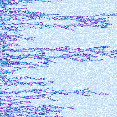
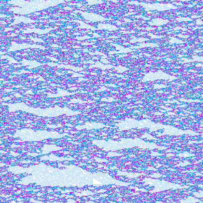
Figure 1: (color online) rule $\mathfrak{110}$, $n=500$. Time goes from left to right, during $500$ steps. Active sites are dark, coalesced site are light (with light blue standing for state $1$, white for $0$). Left: sub-critical phase ($\alpha=0.47<\alpha_{c}\simeq 0.566$), branches die. Right: supercritical phase ($\alpha=0.65>\alpha_{c}$), active sites spread

4.2.1 Measure of $\alpha_{c}$

We use the method described in [4]: plot the density $\rho$ of active sites versus time in logarithmic scale and find the $\alpha$ value for which one gets a straight line (for $\alpha<\alpha_{c}$, the AC coalesce faster, for $\alpha>\alpha_{c}$, it has a positive asymptotic $\rho$). We used random initial configuration with each state equiprobable. To get readable plots we needed up to $n=10^{6}$ cells and $10^{7}$ time steps. We get (recall that $\alpha_{c}$ is not universal, it is just used to compute $\beta$):

rule $\mathfrak{1}$ $\mathfrak{9}_{\ell}$ $\mathfrak{9}_{h}$ $\mathfrak{27}$ $\mathfrak{62}$ $\mathfrak{110}_{\ell}$ $\mathfrak{110}_{h}$ $\mathfrak{126}_{\ell}$ $\mathfrak{126}_{h}$ $\mathfrak{57}$ $\alpha_{c}>\dots$ 0.102 0.073 0.757 0.856 0.598 0.073 0.566 0.101 0.720 0.749 $\alpha_{c}<\dots$ 0.103 0.074 0.758 0.858 0.599 0.075 0.567 0.102 0.721 0.750

Note that the $\alpha_{c}$ of $\mathfrak{1}$ and $\mathfrak{126}_{\ell}$, like $\mathfrak{9}_{\ell}$ and $\mathfrak{110}_{\ell}$, are very close.

4.2.2 Measure of $\beta$

We now plot $\rho$ vs $\alpha$ (fig. 2). The assumption $\rho=c\,(\alpha-\alpha_{c})^{\beta}$ is valid only near $\alpha_{c}$. To determine which points should be taken into account, we plot $\rho(\alpha)$ on a logarithmic scale with $x$-origin roughly equal to $\alpha_{c}$ (precision does not affect the result). We keep only the beginning of the curve which is a straight line. We varied the number of points taken into account to estimate the loss of precision due to this choice.

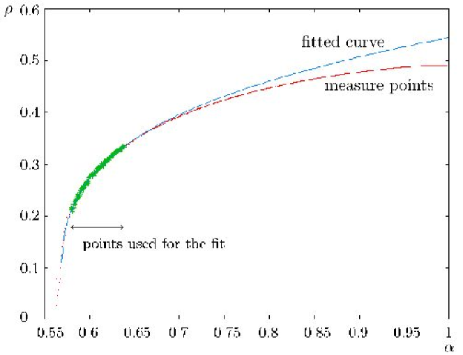
Figure 2: $\rho(\alpha)$. Rule $\mathfrak{110}$, $n=10\,000$. Fitted curve agrees with points used for the fit (bold).

Protocol

$n=10\,000$. We let the system evolve for $T_{\text{tr}}=100\,000$ steps, then measure $\rho$ during $T_{\text{samp}}=10\,000$ step and compute the average. We repeat such a run for each $\alpha$ value with a fine sampling. The fact that the curve is smooth (except very near $\alpha_{c}$) tells us that measures do not depend much on the randomness (nor on $T_{\text{samp}}$) and that we do not need error bars. We also checked that the results do not vary when we change $n$ and $T_{\text{tr}}$.

The fit gives the following ranges, taking into account uncertainty about $\alpha_{c}$ and which points to keep for the fit. Experimental value for $\beta$ measured on other systems is $0.276$.

rule $\mathfrak{1}$ $\mathfrak{9}_{\ell}$ $\mathfrak{9}_{h}$ $\mathfrak{27}$ $\mathfrak{62}$ $\mathfrak{110}_{\ell}$ $\mathfrak{110}_{h}$ $\mathfrak{126}_{\ell}$ $\mathfrak{126}_{h}$ $\mathfrak{57}$ $\beta>\dots$ 0.265 0.270 0.273 0.258 0.270 0.270 0.271 0.250 0.260 0.248 $\beta<\dots$ 0.279 0.295 0.283 0.305 0.281 0.291 0.281 0.276 0.276 0.281

As expected, this model seems to belong to the universality class of directed percolation (except perhaps $\mathfrak{27}$, due to higher noise and thus lack of precision).

Source code is available on cimula.sf.net.

References

- [1] Fatès, N., Morvan, M.: An experimental study of robustness to asynchronism for elementary cellular automata. Complex Systems 16 (2005) (to appear).
- [2] Kaulakys, B., Ivanauskas, F., Mekauskas, T.: Synchronization of chaotic systems driven by identical noise. International Journal of Bifurcation and Chaos 9(3) (1999) 533–539
- [3] Fates, N., Regnault, D., Schabanel, N., Thierry, E.: Asynchronous behavior of double-quiescent elementary cellular automata. In: LATIN. (2006) (to appear).
- [4] Hinrichsen, H.: Nonequilibrium critical phenomena and phase transitions into absorbing states. Advances in Physics (2000) 815