Noise-induced cooperative dynamics and its control in coupled neuron models

Abstract

We investigate feedback control of the cooperative dynamics of two coupled neural oscillators that is induced merely by external noise. The interacting neurons are modelled as FitzHugh-Nagumo systems with parameter values at which no autonomous oscillations occur, and each unit is forced by its own source of random fluctuations. Application of delayed feedback to only one of two subsystems is shown to be able to change coherence and timescales of noise-induced oscillations either in the given subsystem, or globally. It is also able to induce or to suppress stochastic synchronization under certain conditions.

I Introduction

Neural systems in many cases are characterized by oscillatory behavior BRA94 ; LU95 ; EGU00 , which is often quite complicated SOF93 . It has been shown that neural oscillatory dynamics can have different origins, being either self-sustained HOD52 , or induced by random fluctuations alone JUN98 ; BAD05 . These oscillations can also be multimodal, i.e., consisting of several components with different prominent timescales. For example the thalamocortical relay neurons can generate either spindle or $\delta$ oscillations WAN94 , whereas the electro-receptors in a paddle fish are able to generate biperiodic oscillations NEI01 . Coupled neurons are able to demonstrate synchronization, which plays a very important role in neurodynamics, having either constructive, or destructive effects depending on the circumstances.

On one hand, the ensembles of different neurons can be synchronized in order to process biological information, i.e., this synchronization might be beneficial for a more efficient data transmission SAM04 ; BEN04 . On the other hand, these synchronized neurons can induce a regular, rhythmic activity, which is believed to play a crucial role in the emergence of pathological rhythmic brain activity in Parkinson’s disease, essential tremor, and epilepsy TAS98 ; GRO02 . In both situations, synchronization phenomena occur spontaneously, and the mechanisms behind them are the subjects of intensive research GRO02 ; BEN04 . Hence, the development of techniques that would allow one to manipulate the neural synchrony is an important clinical problem.

Starting with the work of Ott, Grebogi and Yorke OTT90 , a variety of methods for the control of irregular behavior have been developed in the last 15 years SCH99c ; BOC00 . Recently, a number of methods have been proposed for suppression of synchrony in the arrays of coupled oscillators in which oscillations are self-sustained ROS04 ; POP05 . However, the problem of control of the dynamics in coupled systems where oscillations are induced merely by random fluctuations is still open.

In this paper we investigate the possibility of using for this purpose the delayed feedback scheme introduced by Pyragas PYR92 : it constructs a control force from the difference between the current state of the system and its state some $\tau$ time units ago. This method is known as time-delay autosynchronization (TDAS). It has been applied to control of deterministic chaos in a wide range of systems including spatially extended models, e.g. BAB02 ; BEC02 ; UNK03 . It was also demonstrated that it can be used to control the coherence and the timescales of noise-induced oscillations in a single system JAN04 ; BAL04 ; POM05a . This theoretical prediction has recently been verified experimentally in an electrochemical oscillator system SAN06 . The main aim of the present work is to extend time-delayed feedback control of noise-induced dynamics to coupled excitable systems, and investigate if local control applied to a subsystem can allow one to steer the global cooperative dynamics in a system of coupled neural oscillators. In particular, we are interested in the study of the effects of delayed feedback on the synchrony properties in coupled neuron systems.

The paper is organized as follows. In Section II we introduce the model system used, and discuss the properties of their cooperative behavior without control. In Section III we study the effects of local delayed feedback control on the global behavior of coupled systems. In Section IV the results are summarized and the conclusions are drawn.

II Global dynamics of two coupled neural oscillators

In order to grasp the complicated interaction between billions of neurons in large neural networks, those are often lumped into groups of neural populations each of which can be represented as an effective excitable element that is mutually coupled to the other elements ROS04 ; POP05 . In this sense the simplest model which may reveal features of interacting neurons consists of two coupled neural oscillators. Each of these will be represented by a simplified FitzHugh-Nagumo system, which is often used as a paradigmatic generic model for neurons, or more generally, excitable systems LIN04 . Here we use two FitzHugh-Nagumo systems with substantially different intrinsic timescales, and parameters corresponding to the excitable regime. Before attempting to control their global dynamics with locally applied feedback, we will first study the dynamics of the uncontrolled coupled system. The dynamical equations are given by:

$$\epsilon_{1}\,\dot{x}_{1} = x_{1}-\frac{x_{1}^{3}}{3}-y_{1}+C\,\left(x_{2}-x_{1}\right),$$

$$\dot{y}_{1} = x_{1}+a+D_{1}\,\xi_{1}(t),$$ (1)

$$\epsilon_{2}\,\dot{x}_{2} = x_{2}-\frac{x_{2}^{3}}{3}-y_{2}+C\,\left(x_{1}-x_{2}\right),$$

$$\dot{y}_{2} = x_{2}+a+D_{2}\,\xi_{2}(t),$$ (2)

where subsystems Eqs. (II) and (II) represent two different neurons, $x_{i}$ ($i=1,2$) describing the transmembrane voltages and $y_{i}$ modelling the behavior of several physical quantities related to electrical conductances of the relevant ion currents across the respective membranes. Here $a$ is a bifurcation parameter whose value defines whether the system is excitable or demonstrates periodic firing (autonomous oscillations), $\epsilon_{1}$ and $\epsilon_{2}$ are positive parameters that are usually chosen to be much smaller than unity, $\xi_{1}$ and $\xi_{2}$ are independent sources of Gaussian white noise with zero mean and unity variance, $D_{1}$ and $D_{2}$ are noise intensities.

The synaptic coupling between two neurons is modelled as a diffusive coupling considered for simplicity to be symmetric LIL94 ; PIN00 ; DEM01 . The coupling strength $C$ summarizes how information is distributed between neurons.

We shall restrict our analysis to the range of the parameter values where without noise each of the two subsystems exhibits excitability with only one attractor in the form of a stable fixed point. Noise sources $\xi_{1}$ and $\xi_{2}$ model random inputs that represent integral signals coming from the part of the neural network or of the environment with which the neuron is connected. Since the neurons can be coupled to different parts of the neural network or of the environment, the noise intensities in the two systems can be quite different.

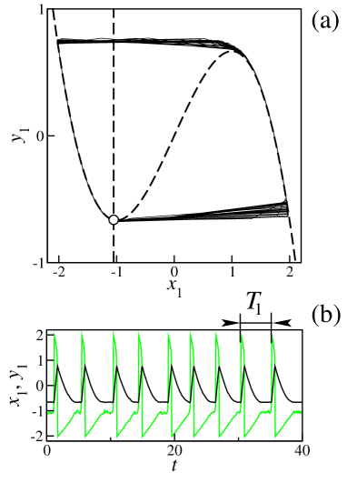
Figure 1: (color online) (a) Phase portrait and (b) realizations of $x_{1}$ (grey, green online) and $y_{1}$ (black) time series in a single FitzHugh-Nagumo system Eq. (II). In (a) dashed lines are null-clines and the fixed point is shown by a white circle. Parameters: $a$$=$$1.05$, $\epsilon_{1}$$=$$0.005$, $D_{1}=0.02$.

II.1 Features of a single neuron model

Let us illustrate the dynamics of a single neuron model by considering an uncoupled subsystem Eqs. (II) ($C$$=$$0$) under the influence of noise. We arbitrarily fix $D_{1}$$=$$0.02$, and also set $a=1.05$, $\epsilon_{1}$$=$$0.005$. In Fig. 1(a) dashed lines show the null-clines of Eq. (II) that intersect at a fixed point marked by a white circle. The phase point that is initially placed at the fixed point stays in its close vicinity if the applied random perturbation remains small. However, if the perturbation is larger than some threshold value, the phase point makes a large excursion in the phase space before returning to the vicinity of the fixed point again. In Fig. 1(a) the black solid line illustrates a phase portrait and in Fig. 1(b) realizations of $x_{1}$ and $y_{1}$ time series from Eqs. (II) are shown. The motion of the phase point consists of two stages: an activation time during which the system waits for a sufficiently large perturbation before it can make an excursion, and the excursion itself. The excursion time is almost completely defined by the deterministic properties of the system and is hardly influenced by noise.

On the contrary, the activation time is completely determined by the properties of noise if all other parameters are fixed: the stronger the noise, the smaller the activation time and the larger the mean frequency of noise-induced oscillations is. Thus, the noise strengths $D_{1}$ and $D_{2}$ control the average frequencies of noise-induced oscillations in the systems Eqs. (II) and (II), respectively, and the difference between them defines the mean frequency detuning between the systems.

II.2 Means for characterizing cooperative dynamics

Before studying the effects of delayed feedback control on the model Eqs. (II) and (II), let us examine the basic features of cooperative dynamics of two systems in which oscillations are induced merely by noise.

The cooperative dynamics of a system of coupled stochastic oscillators can be characterized differently depending on the feature of interest. The most popular features are timescales involved, degree of order in each partial subsystem and in the system of coupled oscillators as a whole, and the degree of synchronism between the subsystems. To quantitatively characterize each feature of interest, a number of criteria can be used, and here we will choose those that seem to suit best our purposes.

Timescales. The Fourier power spectral density, to which in the following we will refer as spectrum for brevity, seems to be the most universal and sensitive tool that allows one to fully reveal the frequency content of random oscillations and thus characterize the timescales involved. The central frequencies of the highest spectral peaks will characterize the timescales involved.

Another convenient and less computationally expensive way to characterize the timescales of oscillations is to introduce the interspike intervals (ISI) $T_{1}$ and $T_{2}$ for the two systems from their realizations $x_{1}(t)$ and $x_{2}(t)$, respectively, as shown in Fig. 1(b). The average ISIs $\langle T_{i}\rangle$, $i=1,2$, will also characterize the timescales of two systems.

Coherence. Generally, the width of the spectral peak can serve as an indication of the coherence of the oscillations: the narrower the peak is, the more coherent the oscillations are. However, as we will see below, the spectra of the observed oscillations have several distinguishable peaks with comparable heights placed at incommensurate frequencies (i.e., at frequencies that are not multiples of each other), and all peaks have different widths. It is not obvious the width of which peak should be taken as a measure of coherence, and thus the peak width does not represent an unambiguous criterion here and will not be used.

Another measure of coherence of oscillations is the correlation time $t_{cor}$. It is also not unambiguous because it can be introduced in several ways. Here we will use the following method which seems the most universal: an autocorrelation function $\Psi(s)=\langle[x(t-s)-\langle x\rangle][x(t)-\langle x\rangle]\rangle$ will be calculated from the simulated realizations $x(t)$, and $t_{cor}$ will be introduced as

$$t_{cor}=\frac{1}{\sigma^{2}}\int_{0}^{\infty}|\Psi(s)|\,ds,$$ (3)

where $\sigma^{2}=$ $\Psi(0)$ is the variance of $x(t)$. The larger $t_{cor}$ is, the more regular $x(t)$ is.

Timescales and coherence can be introduced for each subsystem separately and then compared, or for some variable characterizing the state of the system as a whole. Thus, we will estimate the statistical characteristics of the variables $x_{1}$ and $x_{2}$, and of the global state variable $x_{\Sigma}=x_{1}+x_{2}$.

Synchronization. Finally, we need to characterize the synchronization between the two coupled oscillators. Most generally, synchronization means an adjustment of timescales of oscillations in systems due to the interaction between them: if the timescales in the uncoupled systems are not rationally related, introduction of coupling can shift the timescales to make their ratio closer to a rational number $n$$:$$m$, where $n$ and $m$ are integers. This phenomenon is usually referred to as $n$$:$$m$ frequency synchronization, and its suitable measure would be the closeness of the ratio of average ISIs $\langle T_{1}\rangle$$/$$\langle T_{2}\rangle$ to the chosen rational number $n$$:$$m$. Note that frequency synchronization is associated with the time-averaged behavior of the coupled oscillators.

A closely related, but not identical, phenomenon, which is usually called phase synchronization, is associated with instantaneous coordination between the interacting systems. It requires the definition of phases $\varphi_{1}(t)$ and $\varphi_{2}(t)$ for each oscillator and comparison between them. In our system the spiky nature of oscillations allows one to introduce the phase for each system as:

$$\varphi_{j}(t)=2\pi\frac{t-t_{i-1}}{t_{i}-t_{i-1}}+2\pi(i-1),\,\,j=1,2,...,$$ (4)

where $t_{i}$ is the time at which we observe a spike in the respective system’s realization.

We define $n$$:$$m$ phase synchronization to occur if the phase difference

$$\Delta\varphi_{n,m}(t)=\varphi_{1}(t)-\frac{m}{n}\varphi_{2}(t),$$ (5)

exhibits horizontal plateaus of sufficient duration. Usually, if $n$$:$$m$ synchronization takes place, $\Delta\varphi_{n,m}(t)$ demonstrates plateaus occasionally interrupted by $2\pi$ jumps. On the plateaus, $\Delta\varphi_{n,m}(t)$ usually oscillates around some local average level. As time grows, $\Delta\varphi_{n,m}(t)$ drifts to plus or minus infinity.

In Ros_Moss_book several measures to characterize phase synchronization were introduced. Here, we choose to estimate the synchronization index

$$\gamma_{n,m}=\sqrt{\langle\cos\Delta\varphi_{n,m}(t)\rangle^{2}+\langle\sin\Delta\varphi_{n,m}(t)\rangle^{2}}.$$ (6)

$\gamma_{n,m}$ can vary between $0$ (no synchronization) and $1$ (perfect $n$$:$$m$ phase synchronization). Note that even if the ratio of average ISIs is close or even equal to some rational number $n$$:$$m$, i.e., frequency synchronization takes place, phase synchronization does not necessarily occur, and the synchronization index might be close to zero.

II.3 Cooperative noise-induced dynamics in two coupled neurons: timescales and coherence

All results in this paper are presented for $a$$=$$1.05$, $\epsilon_{1}$$=$$0.005$, $\epsilon_{2}$$=$$0.1$, and $D_{2}=0.09$. Mean frequency detuning will be determined by the choice of $D_{1}$. Note that $\epsilon_{1}\neq\epsilon_{2}$, i.e. the systems are not identical, therefore at $D_{1}=D_{2}$ the mean frequencies of oscillations in two uncoupled ($C=0$) systems will be different.

We need to find out how the cooperative dynamics of the interacting systems changes depending on coupling strength $C$ and on the mean frequency detuning defined by $D_{1}$.

We first fix the coupling strength $C$ at $0.07$, and change $D_{1}$. Fig. 2 shows the realizations $x_{1}$, $x_{2}$ and $x_{\Sigma}$ of noise-induced oscillations. At $D_{1}$$=$$0$ the first subsystem, whose variables are denoted by subscript 1 in Eq. (II), has no independent dynamics. But due to the coupling with the second subsystem, it demonstrates forced oscillations whose properties are completely defined by those of the second subsystem. The respective realizations of $x_{1}$ and $x_{2}$ demonstrate excellent synchrony, so that each spike in $x_{2}$ causes a spike in $x_{1}$ that occurs simultaneously (Fig. 2 ($D_{1}$$=$$0$)).

At $D_{1}\neq 0$ the first subsystem acquires its own dynamics with the respective independent timescale. Now each time one of the subsystems produces a noise-induced spike, due to coupling the other subsystem is prompted to spike, too: it does not necessarily emit a spike, but the spiking probability grows slightly. As a result, both subsystems are likely to spike slightly more frequently (Fig. 2 ($D_{1}$$=$$0.05$)) This is reflected by the decrease of respective average ISIs in Fig. 3(a). As $D_{1}$ grows further, the mean frequency of spiking in the first subsystem grows in agreement with Lind_CR_99 . However, coupling is small here, so the second subsystem only rarely responds with a spike to the spike in the first subsystem. As a result, while the spiking frequency in the first subsystem is further increased, the second subsystem’s frequency stays almost constant (Fig. 2 ($D_{1}$$=$$1$) and 3(a)).

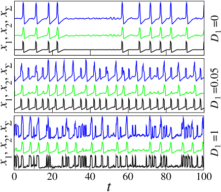
Figure 2: (color online) Realizations of $x_{1}$ (lower), $x_{2}$ (middle) and $x_{\Sigma}=x_{1}+x_{2}$ (upper trace) of noise-induced oscillations in two coupled FitzHugh-Nagumo systems Eqs. (II), (II) for various noise intensities $D_{1}$ in the first system for $C$$=$$0.07$.

The continuous change of timescales and of coherence of the noise-induced dynamics with $D_{1}$ is illustrated in Fig. 3. Here, average ISIs (a) and $t_{cor}$ (b) are shown. The latter are estimated from $x_{1}$ and $x_{2}$ thus quantifying the local dynamics, and from $x_{\Sigma}$$=$$x_{1}$$+$$x_{2}$ thus characterizing the global behavior.

All three graphs for $t_{cor}$ show clear maxima which can be regarded as occurrence of coherence resonance (CR) PIK97 . However, in different systems CR occurs at different noise intensities $D_{1}$, and the mutual coupling between the two systems leads to the occurrence of two maxima in $t_{cor}$ calculated from $x_{2}$.

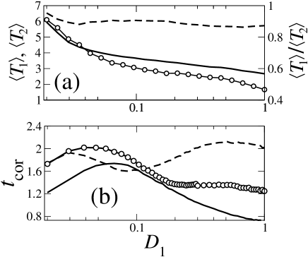
Figure 3: Timescales and coherence of noise-induced oscillations in two coupled FitzHugh-Nagumo systems Eqs. (II) and (II) vs $D_{1}$ at $C$$=$$0.07$. (a) Average ISIs $\langle T_{1}\rangle$ (solid line), $\langle T_{2}\rangle$ (dashed line) and their ratio (circles). (b) Correlation time $t_{cor}$ obtained from $x_{1}$ (solid line), $x_{2}$ (dashed line) and $x_{\Sigma}$ (circles). See text for details.

Now consider how noise-induced dynamics changes with variation of the coupling $C$ between neurons. We choose $D_{1}$$=$$0.25$, so that without coupling ($C$$=$$0$) the oscillations in the two systems have essentially different timescales with $\langle T_{1}\rangle\approx 3.25$ and $\langle T_{2}\rangle\approx 8.1$. At $C$$=$$0$ the two subsystems oscillate independently (Fig. 4, top panel). As the coupling is increased from zero, the subsystems start to experience each others’ influence: each time one system spikes, the other is prompted to spike, too (Fig. 4, middle panel). This results in timescales moving closer (Fig. 3(a)). As the coupling grows further, the two subsystems spike more simultaneously (Fig. 4, bottom panel), and their average ISIs tend to coincide. The latter can serve as an evidence for stochastic $1$$:$$1$ frequency synchronization HAN99 , which will be discussed in more detail below.

Figure 4: (color online) Realizations of $x_{1}$ (lower), $x_{2}$ (middle) and $x_{\Sigma}$ (upper trace) of noise-induced oscillations in two coupled FitzHugh-Nagumo systems Eqs. (II) and (II) for various coupling strengths $C$ at $D_{1}$$=$$0.25$.

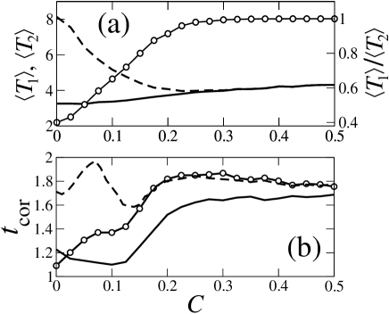
Figure 5: Timescales and coherence of noise-induced oscillations in two coupled FitzHugh-Nagumo systems Eqs. (II) and (II) vs coupling strength $C$ at $D_{1}$$=$$0.25$. (a) Average ISIs $\langle T_{1}\rangle$ (solid line), $\langle T_{2}\rangle$ (dashed line) and their ratio (circles). (b) Correlation time $t_{cor}$ obtained from $x_{1}$ (solid line), $x_{2}$ (dashed line) and $x_{\Sigma}$ (circles). See text for details.

The full dependence of ISIs and $t_{cor}$ on $C$ is shown in Fig. 5. In the absence of coupling, the two systems randomly oscillate, being independent of each other, hence the coherence of the sum signal is less than the coherences of the individual signals. At large $C>0.2$, the global coherence becomes equal to the coherence of the second system, which is more ordered individually than its neighbour.

II.4 Synchronization: frequency (phase) locking and suppression of noise-induced oscillations

Synchronization phenomena in coupled oscillators with noise-induced dynamics were previously considered, e.g. in HAN99 ; POS02 . In contrast to these works, our model consists of essentially non-identical subsystems whose dynamics is defined by independent sources of noise with different strength, which describes a more general class of natural systems.

In this paper we will discuss only $1$$:$$1$ synchronization. Since synchronization means an adjustment of timescales in interacting systems, the ratio of their average ISIs would serve as a good tool for its detection. In Fig. 6(a) the ratio $\langle T_{1}\rangle/\langle T_{2}\rangle$ is shown for a range of coupling strengths $C$ and of noise intensities $D_{1}$. One can clearly see the $1$:$1$ synchronization region (light area), which has a quite recognizable tongue-like shape, i.e., the larger the coupling strength, the wider the synchronization region with respect to $D_{1}$ is.

Figure 6: (color online) (a) Ratio of average interspike intervals $\langle T_{1}\rangle/\langle T_{2}\rangle$ from the two systems, and (b) synchronization index $\gamma_{1,1}$ vs the coupling strength $C$ and noise intensity $D_{1}$. The light (yellow) areas roughly outline the $1$$:$$1$ (a) frequency and (b) phase synchronization tongues.

Next, we explore if phase synchronization accompanies the frequency synchronization. In Fig. 7 the phase difference is shown for $D_{1}$$=$$0.25$: as $C$ is increased from $0.1$ to $0.4$, the plateaus of $\Delta\varphi_{n,m}(t)$ become longer. At $C=0.4$ the coupling is so strong that the plateau exists (almost) infinitely, which means that the two systems are well $1$:$1$ phase synchronized.

The synchronization index $\gamma_{1,1}$ is computed in the whole range of $D_{1}$ and $C$ and is shown in Fig. 6(b). Inside the whole region of $1$:$1$ frequency synchronization where the ISI ratio is close to unity, the phase synchronization index is close to unity, too. Thus, phase synchronization occurs together with frequency synchronization.

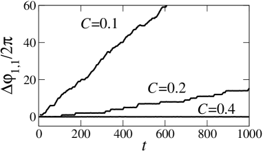
Figure 7: Phase difference $\Delta\varphi_{1,1}$ for the suspected $1$:$1$ synchronization at three different values of coupling strength $C$ and $D_{1}$$=$$0.25$.

It has been known for a long time that synchronization can be achieved via at least two different mechanisms, namely frequency (phase) locking, and suppression of natural dynamics, respectively (see LAN80 for periodic oscillations and MOS02 for chaotic and noise-induced oscillations). We found that in our model both these synchronization mechanisms can be realised, depending on how well the timescales of interacting oscillators were separated from each other when uncoupled. An example of synchronization via frequency (phase) locking is illustrated by Fig. 8(a), where for $D_{1}$$=$$0.25$ the spectra of signal $x_{1}$ and of $x_{2}$ are illustrated for increasing $C$. As $C$ grows, two distinguishable peaks corresponding to the timescales of the two subsystems move closer and then merge. Fig. 8(b) shows how synchronization is realised via the suppression of natural dynamics at $D_{1}$$=$$0.5$. One can see that the increase of $C$ suppresses one of the spectral peaks, i.e. one of the timescales of the system (II). Thus, mutually coupled systems with noise-induced spiking are able not only to demonstrate mutual synchronization itself, but also to reproduce two different synchronization mechanisms, in full analogy with coupled self-oscillating systems.

Figure 8: (Color online) The spectra of $x_{1}$ (black) and $x_{2}$ (shaded grey area, green online) are compared as the coupling strength $C$ is increased for two different strengths of noise in the first subsystem (a) $D_{1}$$=$$0.25$ and (b) $D_{1}$$=$$0.5$. In (a) the highest spectral peaks move towards each other and coincide: frequency (phase) locking. In (b) the highest peak in the spectrum of $x_{1}$ is suppressed, while another peak simultaneously appears and grows at the peak frequency of $x_{2}$: suppresion of natural dynamics.

III Local delayed feedback control of noise-induced cooperative dynamics

In this section we investigate whether the feedback applied only to one of the interacting subsystems, i.e., locally, is able to manipulate the global properties of the system of coupled oscillators. This might simulate a realistic situation where only a small area of the neural network is available for external stimulation. In particular, we will investigate if global timescales, coherence and the strength of synchronization can be influenced.

The time-delayed feedback control proposed by Pyragas PYR92 for control of deterministic chaos was previously applied for the control of noise-induced oscillations in a single system with noise-induced dynamics JAN04 ; BAL04 ; POM05a . It has been demonstrated that it can successfully change the timescales and coherence of oscillations and is thus a promising tool for control of noise-induced phenomena in general.

For our purpose, we apply the time-delayed feedback to the first subsystem alone, while the second system remains freely coupled to it. The feedback force $F(t)$ is constructed as follows: the slow state variable $y_{1}$ is saved at the current time $t$ and at a time $(t-\tau)$, their difference is calculated and multipled by the feedback strength $K$. $F(t)$ is then fed back to the $y$-component of the vector field

$$\epsilon_{1}\,\dot{x}_{1} = x_{1}-\frac{x_{1}^{3}}{3}-y_{1}+C\,\left(x_{2}-x_{1}\right),$$ (7)

$$\dot{y}_{1} = x_{1}+a+K\,[y_{1}(t-\tau)-y_{1}(t)]+D_{1}\,\xi(t),$$

where $\tau$ is the time delay and the other parameters are as in Eqs. (II).

We will be guided by the full picture of cooperative dynamics of the two mutually coupled subsystems that was revealed in Sec. II. We will choose states with different global dynamics by choosing pairs of parameters $D_{1}$ and $C$, and study the effect of the delayed feedback on each state.

We select pairs of points ($D_{1}$, $C$) (see Fig. 6) at which the two systems are (i) far away from ($D_{1}$$=$$0.6$, $C$$=$$0.1$), (ii) closer to ($D_{1}$$=$$0.6$, $C$$=$$0.2$), and (iii) almost inside ($D_{1}$$=$$0.15$, $C$$=$$0.2$) the $1$$:$$1$ synchronization region. In Sec. III.1 we study in detail the case of a moderately synchronized system at $D_{1}$$=$$0.6$ and $C$$=$$0.2$, subject to delayed feedback. We reveal the common features of the feedback effect depending on its parameters $\tau$ and $K$.

Further on, in Sec. III.2, we study two more cases of systems further from, and closer to, the $1$$:$$1$ synchronization region under the delayed feedback action. We compare the effect of the feedback with its effect on a moderately synchronized system.

III.1 Control of a moderately synchronized system

Here, we consider subsystems Eqs. (7) and (II) with $D_{1}$$=$$0.6$ and $C$$=$$0.2$, under the influence of the controlling feedback. We aim to find out if the feedback can make the subsystems more, or less, synchronous, and their global dynamics more or less coherent. In particular, we are interested if perfect $1$$:$$1$ synchronization can be induced by the local feedback, or if the existing synchronization can be destroyed. The ratio of ISIs and the synchronization index $\gamma_{1,1}$ are shown by color code in Fig. 9 for a large range of the values of the feedback delay $\tau$ and strength $K$. The lighter areas are associated with the stronger $1$$:$$1$ synchronization, and the values at $K$$=$$0$ and at $\tau$$=$$0$ characterize the original state of the system without feedback. As seen from Fig. 9, the locally applied delayed feedback is able to move the system’s state closer to the $1$$:$$1$ synchronization with suitable feedback parameters. On the other hand, for $\tau\approx 2.5$ (black area) $1$$:$$1$ synchronization is suppressed.

An illustration of how realizations $x_{1}$, $x_{2}$ and $x_{\Sigma}$ change depending on the feedback strength $K$ as $\tau$$=$$1$ is fixed, is given in Fig. 10, Note that the cut at $\tau$$=$$1$ (Fig. 9) goes through the region where the strongest $1$$:$$1$ synchronization is achieved. As $K$ grows, the oscillations in the two subsystems become more and more synchronized until at $K$$=$$2$ the two systems start to fire simultaneously almost all the time. However, at least in the given range of $K$, the perfect $1$$:$$1$ synchronization, with both ISI ratio and synchronization index equal to unity, is still not realized.

Fig. 11(a) shows the full dependences upon $K$ of $\langle T_{1}\rangle$ (solid line), $\langle T_{2}\rangle$ (dashed line) and of their ratio (circles). In Fig. 11(b) the respective dependences of correlation time $t_{cor}$ from $x_{1}$ (solid line), $x_{2}$ (dashed line) and from the sum signal $x_{\Sigma}$ (circles), are given together with the synchronization index $\gamma_{1,1}$ (grey line, green online). Both $\langle T_{1}\rangle$ and $\langle T_{2}\rangle$ grow monotonically with $K$, which means that at $\tau$$=$$1$ the feedback slows down the oscillations. Within the accuracy of numerical simulation, both ISI ratio and $\gamma_{1,1}$ grow linearly with $K$, still not achieving the value of $1$ at $K$$=$$2$. $t_{cor}$ from $x_{\Sigma}$ grows with $K$ almost linearly as well, which means that the global dynamics of the system becomes more ordered with the stronger feedback. However, $t_{cor}$ computed from $x_{1}$ and $x_{2}$ separately are nonmonotonic.

Figure 9: (color online) Effect of delayed feedback on frequency and phase synchronization betwen the two subsystems at $D_{1}$$=$$0.6$ and $C$$=$$0.2$, which corresponds to a moderate distance from the $1$$:$$1$ synchronization tongue shown in Fig. 6. (a) Ratio of average interspike intervals $\langle T_{1}\rangle/\langle T_{2}\rangle$ from the two systems and (b) synchronization index $\gamma_{1,1}$ vs the control strength $K$ and the time-delay $\tau$.

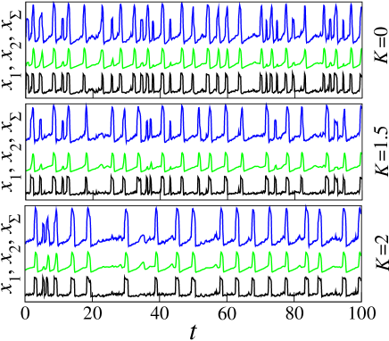
Figure 10: (color online) Realizations of $x_{1}$ (lower), $x_{2}$ (middle) and $x_{\Sigma}$ (upper trace) of noise-induced oscillations in two coupled FitzHugh-Nagumo systems Eqs. (7) and (II) at $D_{1}$$=$$0.6$ and $C$$=$$0.2$, subject to delayed feedback with $\tau=1$ for different values of the feedback strength $K$. See Fig. 11 for reference.

Figure 11: (color online) Timescales, coherence and synchronization index of noise-induced oscillations in two coupled FitzHugh-Nagumo systems Eqs. (7) and (II) vs $K$ of the local feedback at $\tau=1$, $D_{1}$$=$$0.6$ and $C$$=$$0.2$ (see Fig. 9 for reference). (a) Average ISIs $\langle T_{1}\rangle$ (solid line) and $\langle T_{2}\rangle$ (dashed line), and their ratio (circles). (b) Correlation times $t_{cor}$ obtained from $x_{1}$ (solid line), from $x_{2}$ (dashed line), and from $x_{\Sigma}$ (circles). Synchronization index $\gamma_{1,1}$ (grey line, green online).

Next, we follow the route with a constant $K$$=$$1.5$ that crosses the area with the strongest synchronization, by changing $\tau$. Four respective realizations from the subsystems are shown in Fig. 12. A full picture showing ISIs, their ratio, correlation times and synchronization index vs $\tau$ is given in Fig. 13. Both $\langle T_{1}\rangle$ and $\langle T_{2}\rangle$, as well as their ratio, change nonmonotonically with $\tau$ while its value is smaller than $8$. At $\tau>8$ they start to asymptotically tend to some constant values that are slightly larger than those without feedback.

An increase of $\tau$ from zero leads to an increase of both $\langle T_{1}\rangle$ and $\langle T_{2}\rangle$. But $\langle T_{1}\rangle$ grows faster than $\langle T_{2}\rangle$, thus their ratio $\langle T_{1}\rangle$$/$$\langle T_{2}\rangle$ grows with $\tau$, as well as the phase synchronization index $\gamma_{1,1}$. At the same time, the coherence of each subsystem and of their global dynamics grows, too, as illustrated by the behavior of the respective correlation times $t_{cor}$ (Fig. 13(b)).

After the maximum of $\langle T_{1}\rangle$ and $\langle T_{2}\rangle$, and of their ratio, is achieved at $\tau$$\approx$$0.7$, both $\langle T_{1}\rangle$ and $\langle T_{2}\rangle$ start to decrease, but again $\langle T_{1}\rangle$ decreases faster than $\langle T_{2}\rangle$, thus their ratio decreases. A similar behavior is observed in $t_{cor}$ and in $\gamma_{1,1}$.

Starting from $\tau$$\approx$$2$, the ISI $\langle T_{1}\rangle$ of the first system hardly changes with $\tau$. However, counterintuitively, the ISI $\langle T_{2}\rangle$ of the second system responds to the further increase of $\tau$ by displaying a noticeable maximum at $\tau$$\approx$$2.5$. This leads to a well-pronounced minimum of the ISI ratio (Fig. 13(a)) and of the synchronization index $\gamma_{1,1}$ (Fig. 13(b)). This phenomenon is accompanied by a respective maximum of the coherence of the second susbystem and of the global dynamics, while neither the timescales nor the coherence of the first subsystem change substantially. This is a highly counterintuitive phenomenon, since the feedback is applied to the first subsystem only, while the second subsystem responds to the changes of the feedback only indirectly through its coupling with the first subsystem.

With the further increase of $\tau$, the dynamics of the second subsystem changes more substantially than the one of the first subsystem, and thus gives a larger contribution to the changes of the global dynamics.

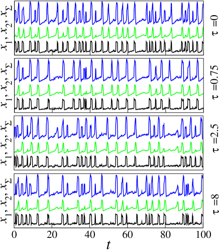
Figure 12: (color online) Realizations of $x_{1}$ (lower), $x_{2}$ (middle) and $x_{\Sigma}$ (upper trace) of noise-induced oscillations in two coupled FitzHugh-Nagumo systems Eqs. (7) and (II) at $D_{1}$$=$$0.6$ and $C$$=$$0.2$, subject to delayed feedback with $K$$=$$1.5$ for different values of the time delay $\tau$. See Fig. 13 for reference.

Figure 13: Timescales, coherence and synchronization index of noise-induced oscillations in two coupled FitzHugh-Nagumo systems Eqs. (7) and (II) vs time delay $\tau$ at $K=1.5$, $D_{1}$$=$$0.6$ and $C$$=$$0.2$ (see Fig. 9 for reference). Symbols as in Fig. 11.

III.2 Control of a weakly, and of a strongly, synchronized system

In this subsection we consider subsystems Eqs. (7) and (II) that are either further from ($D_{1}$$=$$0.6$, $C$$=$$0.1$), or closer to ($D_{1}$$=$$0.15$, $C$$=$$0.2$), the $1$$:$$1$ synchronization region, under the influence of the controlling feedback.

For $D_{1}$$=$$0.6$, $C$$=$$0.1$, the ratio of ISIs and the synchronization index $\gamma_{1,1}$ are shown by color code in Figs. 14. As with the stronger synchronized subsystems, the feedback is able to move the whole system towards a more synchronous state.

As with the example of Sec. III.1, we consider the cut of the $\tau$–$K$ plane along $K=1.5$, choosing the route that goes through the lighter area of the largest synchronization index. ISIs, their ratio, correlation times, and synchronization index are shown in Fig. 15 depending on $\tau$. Their behavior has some similarities to that in a moderately synchronized system of Sec. III.1.

Namely, the initial increase of $\tau$ from zero leads to the growth of both $\langle T_{1}\rangle$ and $\langle T_{2}\rangle$, the former growing faster than the latter. This leads to the growth of the ISI ratio and of synchronization index $\gamma_{1,1}$, and also of $t_{cor}$ of $x_{1}$ and of $x_{\Sigma}$. All variables achieve the maximum at $\tau$$\approx$$0.6$. After that, all the variables describing the first system start to decrease, while $\langle T_{2}\rangle$ does not change until $\tau$$=$$1.5$. Here, the ISI ratio decreases correspondingly, like for $C$$=$$0.2$. And again, after $\tau$$=$$2$, $\langle T_{1}\rangle$ hardly changes with $\tau$, while $\langle T_{2}\rangle$ exhibits a noticeable maximum that leads to the rapid drop of both ISI ratio and synchronization index.

With further increase of $\tau$ beyond $6$, both subsystems respond only slightly and comparably to the changes in $\tau$.

Note that either for a moderately synchronized system, or for a system that is less synchronized, the feedback is able to make $1$$:$$1$ synchronization substantially stronger for a suitable choice of its parameters. However, it cannot destroy the existing synchronization or weaken it as much as it can strengthen it.

Figure 14: (color online) Effect of delayed feedback on frequency and phase synchronization betwen the two subsystems at $D_{1}$$=$$0.6$ and $C$$=$$0.1$, which are further away from the $1$$:$$1$ synchronization tongue shown in Fig. 6, than those considered in Fig. 9. Plot as in Fig. 9.

Figure 15: Timescales, coherence and synchronization index of noise-induced oscillations in two coupled FitzHugh-Nagumo systems Eqs. (7) and (II) depending on the time delay $\tau$ at $K=1.5$, $D_{1}$$=$$0.6$ and $C$$=$$0.1$ (see Fig. 14 for reference). Symbols as in Fig. 11.

For the system that is very well synchronized from the beginning at $D_{1}$$=$$0.15$ and $C$$=$$0.2$ with $\gamma_{1,1}$$=$$0.99$, we reveal the ISI ratio and synchronization index $\gamma_{1,1}$ for a large range of $K$ and $\tau$ (Fig. 16). Already this picture shows that delayed feedback can either enhance or suppress synchronization.

For a more detailed picture of the phenomena induced by the feedback, a cut of this picture along $K$$=$$1$ is given in Fig. 17 where the ISIs and their ratio are shown, together with $\gamma_{1,1}$ and correlation times for $x_{1}$, $x_{2}$ and $x_{\Sigma}$. An immediate obvious observation is that, in contrast to the two previously considered cases of less synchronous subsystems, here the feedback can make synchronization perfect with $\gamma_{1,1}$$=$$1$, and can maintain it like this for a substantial range of $\tau$$\in$$[0.25;2]$ (Fig. 17(a)). The fact that the two subsystems are very synchronous from the beginning is also supported by very similar values of the correlation times of both systems’ realizations and of their sum at $\tau$$=$$0$ (Fig. 17(b)).

As $\tau$ is slighly increased from zero, as in the two previous examples, both $\langle T_{1}\rangle$ and $\langle T_{2}\rangle$ grow. But, as before, $\langle T_{1}\rangle$ grows a little faster than $\langle T_{2}\rangle$. This can hardly be resolved in the plots, since $\langle T_{1}\rangle$ and $\langle T_{2}\rangle$ are very close and hardly distinguishable. However, the difference between them, and the disapperanace of this difference, is visible through the ISI ratio (Fig. 17(a)).

With this, $t_{cor}$ and $\gamma_{1,1}$ slightly grow, too. All quantities considered achieve their maxima at $\tau$$\approx$$0.25$. After that, as $\tau$ increases, the individual ISIs $\langle T_{1}\rangle$ and $\langle T_{2}\rangle$ grow simultaneously and remain equal, so that their ratio and synchronization index $\gamma_{1,1}$ stay equal to $1$ with high accuracy in the range $\tau$$\in$$[0.25;2]$.

However, surprisingly, while the ISI ratio and $\gamma_{1,1}$ are equal to $1$, i.e., the subsystems maintain the same level of perfect synchrony, all three correlation times decrease with $\tau$. This means that while the two subsystems fire simultaneously, these firings occur less regularly. Thus, the feedback here can introduce disorder into the system without destroying its perfect synchronization.

Then, as $\tau$ continues to increase beyond the value of $2$, as in the previous examples, the second subsystem demonstrates a noticeable maximum of its ISI $\langle T_{2}\rangle$. Although unlike in the two other examples, here $\langle T_{1}\rangle$ continues to decrease, the ISI ratio and $\gamma_{1,1}$ exhibit a sharp minimum, and then grow again.

At $\tau$ increases beyond $8$, the ISI ratio and $\gamma_{1,1}$ become less and less dependent on $\tau$, asymptotically tending to some values that are only slighly lower than without the feedback. On the contrary, $t_{cor}$ continues to change nonmonotonically with $\tau$, never becoming less than without the feedback. Since the system is in the state of a strong synchronization throughout the changes in $\tau$, the changes in all three curves $t_{cor}$ occur synchronously.

Thus, the feedback can make both local and global dynamics of the system more coherent, and at the same time weaken synchronization.

Figure 16: (color online) Effect of delayed feedback on frequency and phase synchronization betwen the two subsystems at $D_{1}$$=$$0.15$ and $C$$=$$0.2$, which are closer to the $1$$:$$1$ synchronization tongue shown in Fig. 6, than those considered in Fig. 9. Plot as in Fig. 9.

Figure 17: Timescales, coherence and synchronization index of noise-induced oscillations in two coupled FitzHugh-Nagumo systems Eqs. (7) and (II) depending on the time delay $\tau$ at $K=1$, $D_{1}$$=$$0.15$ and $C$$=$$0.2$ (see Fig. 16 for reference). Symbols as in Fig. 11.

IV Summary and Conclusions

We have considered a model describing two coupled excitable neurons, in the form of two mutually coupled non-identical excitable FitzHugh-Nagumo systems, subject to independent sources of noise with different strengths. In order to assess the effect of time-delayed feedback control upon the coupled system, we have analyzed the following characteristics: the timescales of the individual systems quantified as mean interspike intervals (ISI); the ISI ratio as a measure of frequency synchronization; the coherence quantified by the correlation time of the individual subsystems’ realizations and of their sum; and the index of $1$$:$$1$ phase synchronization between the subsystems.

The coupled system without control displays a $1$$:$$1$ synchronization tongue in the $(D_{1},C)$ parameter plane, given by the noise strength $D_{1}$ in the first subsystem and the coupling strength $C$. Interestingly, frequency and phase synchronization occurred in the same area of the parameter plane. Two mechanisms for synchronization were identified: phase (frequency) locking, and suppression of natural dynamics, respectively.

Next, the first of the two interacting subsystems was subjected to the local delayed feedback with the aim to manipulate the global dynamics of the system of interacting oscillators. The feedback force was constructed as a difference between the current state of the system and its state some $\tau$ time units before, multiplied by a positive constant $K$.

The delayed feedback was applied to the system in three states of synchrony: moderately synchronized, weakly synchronized, and strongly synchronized. In all three cases, $1$$:$$1$ synchronisation could be either improved or weakened, depending upon the choice of $\tau$ and $K$. Like the correlation times, the synchronisation index is modulated nonmonotonically as a function of the delay time $\tau$, indicating that there is resonance-like behavior for certain values of $\tau$. Perfect synchronisation can only be achieved if the uncontrolled state is already sufficiently synchronized.

The mechanism behind the reported action of the delayed feedback is as follows. As it was shown earlier JAN04 ; BAL04 , the feedback applied to a single excitable system is able to change the timescales and coherence of noise-induced oscillations. When the system subjected to the feedback is coupled to another system, the shift of the timescale of the former will lead to a proportional shift of the timescale of the latter. The exact magnitude of the shift in the second subsystem will depend on the closeness of the two subsystems to the state of synchronization. Only if the two subsystems are sufficiently $1$$:$$1$ synchronized from the beginning, the shift in the second system can be expected to match the shift in the first system.

Interestingly, the above mechanism does not always work in the system considered. Namely, for some ranges of time delay $\tau$, the change in $\tau$ does not cause any noticeable change in the system to which the feedback is applied. However, it does change the properties of oscillations in the system that is coupled to it, albeit that does not experience the influence of the feedback directly.

An important observation is that the delay-induced increase of coherence of the global dynamics is most frequently accompanied by the growth of the degree of synchronization. However, a high synchonization index does not always mean high coherence: delayed feedback can induce, or make stronger, the synchronization between the two subsystems, but the state of each subsystem, and their global dynamics, can become more disordered at the same time. The converse is also true.

It is remarkable that delayed feedback control can influence global characteristics of the two coupled neurons although the control is only applied locally to a subsystem. We were able to enhance or destroy the regularity of oscillations and the stochastic synchronization of the two neurons by choosing appropriate control parameters, in particular a suitable delay time.

We consider these findings as important for the understanding of coupled nonlinear systems and see possible applications especially in neuroscience. In fact, experimental studies of two coupled neurons from the stomatogastric ganglion of a lobster PIN00 , and from a leech DEM01 have reported various degrees of synchrony of excitatory postsynaptic potentials. As stochastic sources of the spontaneous random firing of neurons, noise due to the conducting ion channels, synaptic noise, and noise resulting from the coupling to a large number of other neurons emitting signals, have been identified ZEN04 . Also it was demonstrated experimentally JUN98 that spatially and temporally coherent $Ca^{2+}$ waves, mediated by network noise, may play an important role in generating correlated neural activity. By applying delayed feedback control to real neural systems one should be able to influence neural synchrony. First results of applying time-delayed neurofeedback from realtime MEG signals to humans via visual stimulation in order to suppress the alpha rhythm, which is observed due to strongly synchronized neural populations in the visual cortex in the brain, look promising TASS06 . Further work should focus on more sophisticated models and on coupling more than two neurons.

V Acknowledgments

This work was partially supported by DFG in the framework of Sfb 555 (Complex nonlinear processes). B.H. thanks the Studienstiftung des deutschen Volkes for support and gratefully acknowledges the hospitality of Loughborough University. A.B. acknowledges the support of EPSRC (UK).

References

- (1) H. A. Braun, H. Wissing, K. Schäfer, and M. C. Hirsch, Nature 367, 270 (1994).
- (2) J. Lu and H. M. Fishman, Biophys. J. 69, 2458 (1995).
- (3) V. M. Eguiluz, M. Ospeck, Y. Choe, A. J. Hudspeth, and M. O. Magnasco, Phys. Rev. Lett. 84, 5232 (2000).
- (4) W.R. Softky, C. Koch, J. Neurosci. 13, 334 (1993).
- (5) A.L. Hodgkin and A.F. Huxley, J. Physiol. London 117, 500 (1952).
- (6) P. Jung, A. Cornell-Bell, K.S. Madden, and F. Moss, J. Neurophysiol. 79, 1098 (1998).
- (7) M. Badoual, M. Rudolph, Z. Piwkowska, A. Destexhe, and T. Bal, Neurocomp. 65, 493 (2005).
- (8) X.-J. Wang, Neuroscience 59, 21 (1994).
- (9) A. Neiman and D. F. Russell, Phys. Rev. Lett. 86, 3443 (2001).
- (10) J.M. Samonds, J.D. Allison, H.A. Brown, and A.B. Bonds, Proc. Natl. Acad. Sci. USA 101, 6722 (2004).
- (11) A. Benucci, P. F. M. J. Verschure, and P. König, Phys. Rev. E 70, 051909 (2004).
- (12) P. Tass, M. G. Rosenblum, J. Weule, J. Kurths, A. Pikovsky, J. Volkmann, A. Schnitzler, and H.-J. Freund, Phys. Rev. Lett. 81, 3291 (1998).
- (13) P. Grosse, M. J. Cassidy, P. Brown, Clinical Neurophysiology 113, 1523 (2002).
- (14) E. Ott, C. Grebogi, and J. A. Yorke, Phys. Rev. Lett. 64, 1196 (1990).
- (15) H. G. Schuster (Ed.), Handbook of Chaos Control (Wiley-VCH, Weinheim, 1999).
- (16) S. Boccaletti, C.Grebogi, Y. C. Lai, H. Mancini, and D. Maza, Physics Reports 328, 103 (2000).
- (17) M. G. Rosenblum and A. S. Pikovsky, Phys. Rev. E 70, 041904 (2004).
- (18) O.V. Popovych, C. Hauptmann, P.A. Tass, Phys. Rev. Lett. 94, 164102 (2005).
- (19) K. Pyragas, Phys. Lett. A 170, 421 (1992).
- (20) N. Baba, A. Amann, E. Schöll, and W. Just, Phys. Rev. Lett. 89, 074101 (2002).
- (21) O. Beck, A. Amann, E. Schöll, J.E.S. Socolar, and W. Just, Phys. Rev. E 66, 016213 (2002).
- (22) J. Unkelbach, A. Amann, W. Just, and E. Schöll, Phys. Rev. E 68, 026204 (2003).
- (23) N. B. Janson, A. G. Balanov, and E. Schöll, Phys. Rev. Lett. 93, 010601 (2004).
- (24) A. G. Balanov, N. B. Janson, and E. Schöll, Physica D 199, 1 (2004).
- (25) J. Pomplun, A. Amann, and E. Schöll, Europhys. Lett. 71, 366 (2005).
- (26) G. J. Escalera Santos, J. Escalona, and P. Parmananda, Phys. Rev. E 73, 042102 (2006).
- (27) B. Lindner, J. García-Ojalvo, A. Neiman, and L.Schimansky-Geier, Phys. Rep. 392, 321(2004).
- (28) D. T. J. Liley and J. J. Wright, Network Comp. Neur. Systems 5, 175 (1994).
- (29) R. D. Pinto, P. Varona, A. R. Volkovskii, A. Szücs, H. D. I. Abarbanel and M. I. Rabinovich, Phys. Rev. E 62, 2644 (2000).
- (30) F. F. De-Miguel, M. Vargas-Caballero, and E. Garcia-Perez, J. Exp. Biol. 204, 3241 (2001).
- (31) M.G. Rosenblum, A.S. Pikovsky, J. Kurths, C. Schäfer, and P. Tass, In: Handbook of Biological Physics (Elsevier Science, Amsterdam, 2001), Vol. 4, Neuro-informatics and Neural Modeling, Eds. F. Moss and S. Gielen, Ch. 9, 279-321.
- (32) B. Lindner, L. Schimansky-Geier, Phys. Rev. E 60, 7270 (1999).
- (33) A.S. Pikovsky and J. Kurths, Phys. Rev. Lett. 78, 775 (1997).
- (34) S.K. Han, T.G. Yim, D.E. Postnov, and O.V. Sosnovtseva, Phys. Rev. Lett. 83, 1771 (1999).
- (35) D. E. Postnov, O. V. Sosnovtseva, S. K. Han, and W. S. Kim, Phys. Rev. E 66, 016203 (2002).
- (36) P. Landa, Self-oscillations in the systems with finite number of degree of freedom (Nauka, Moscow, 1980) (in Russian).
- (37) E. Mosekilde, Yu. Maistrenko, and D. Postnov, Chaotic synchronization. Applications to Living Systems, World Scientific, Singapore, Series A, Vol. 42 (2002).
- (38) S. Zeng and P. Jung, Phys. Rev. E 70, 011903 (2004).
- (39) V. Hadamschek, PhD Thesis, TU Berlin (2006).