also at ]Jawaharlal Nehru Centre For Advanced Scientific Research, Jakkur, Bangalore, India.

Manifestations of Drag Reduction by Polymer Additives
in Decaying, Homogeneous, Isotropic Turbulence

Abstract

The existence of drag reduction by polymer additives, well established for wall-bounded turbulent flows, is controversial in homogeneous, isotropic turbulence. To settle this controversy we carry out a high-resolution direct numerical simulation (DNS) of decaying, homogeneous, isotropic turbulence with polymer additives. Our study reveals clear manifestations of drag-reduction-type phenomena: On the addition of polymers to the turbulent fluid we obtain a reduction in the energy dissipation rate, a significant modification of the fluid energy spectrum especially in the deep-dissipation range, a suppression of small-scale intermittency, and a decrease in small-scale vorticity filaments.

The dramatic reduction of drag by the addition of small concentrations of polymers to a turbulent fluid continues to engage the attention of engineers and physicists. Significant advances have been made in understanding drag reduction both experimentally vir75 ; dam94 ; too97 and theoretically lum73 ; sre00 ; pta03 ; lvo04 in channel flows or the Kolmogorov flow bof05 . However, the existence of drag-reduction-type phenomena in turbulent flows that are homogeneous and isotropic tab86 ; bha91 ; ben03 ; ben04 ; kal_poly04 ; ang05 ; doo99 ; mcc77 ; fri70 ; bon93 ; bon05 remains controversial. Some experimental doo99 ; mcc77 ; fri70 ; bon93 , numerical ben03 ; ben04 ; kal_poly04 ; ang05 , and theoretical tab86 ; bha91 studies have suggested that drag reduction should occur even in homogeneous, isotropic turbulence; but other studies have refuted this claim bon05 .

To settle this controversy we have initiated an extensive direct numerical simulation (DNS) of decaying, homogeneous, isotropic turbulence in the presence of polymer additives. We monitor the decay of turbulence from initial states in which the kinetic energy of the fluid is concentrated at small wave vectors; this energy then cascades down to large wave vectors where it is dissipated by viscous effects; the energy-dissipation rate $\epsilon$ attains a maximum at $t_{m}$, roughly the time at which the cascade is completed. A recent shell-model study kal_poly04 has suggested that this peak in $\epsilon$ can be used to quantify drag reduction by polymer additives. Since shell models are far too simple to capture the complexities of real flows, we have studied decaying turbulence in the Navier-Stokes (NS) equation coupled to the Finitely Extensible Nonlinear Elastic Peterlin (FENE-P) model pet66 for polymers. Our study, designed specifically to uncover drag-reduction-type phenomena, shows that the position of the maximum in $\epsilon$ depends only mildly on the polymer concentration $c$; however, the value of $\epsilon$ at this maximum falls as $c$ increases. We use this decrease of $\epsilon$ to define the percentage drag (or dissipation) reduction DR in decaying homogeneous, isotropic turbulence; we also explore other accompanying physical effects and show that they are in qualitative accord with drag-reduction experiments bon93 ; hoy77 : In particular, DR increases with $c$ (upto $25\%$ in one of our simulations). For small values of $c$ the energy spectrum of the fluid is modified appreciably only in the dissipation range; however, this suffices to yield significant drag reduction. We show that vorticity filaments and intermittency are reduced at small spatial scales and that the extension of the polymers decreases as $c$ increases.

The NS and FENE-P (henceforth NSP) equations are

$$D_{t}{\bf u} = \nu\nabla^{2}{\bf u}+\frac{\mu}{\tau_{P}}\nabla.[f(r_{P}){\cal C}]-{\nabla}p;$$ (1)

$$D_{t}{\cal C} = {\cal C}.(\nabla{\bf u})+{(\nabla{\bf u})^{T}}.{\cal C}-\frac{{f(r_{P}){\cal C}}-{\cal I}}{\tau_{P}}.$$ (2)

Here ${{\bf u}({\bf x},t)}$ is the fluid velocity at point ${\bf x}$ and time $t$, incompressibility is enforced by $\nabla.{\bf u}=0$, $D_{t}=\partial_{t}+{\bf u}.\nabla$, $\nu$ is the kinematic viscosity of the fluid, $\mu$ the viscosity parameter for the solute (FENE-P), $\tau_{P}$ the polymer relaxation time, $\rho$ the solvent density (set to $1$), $p$ the pressure, $(\nabla{\bf u})^{T}$ the transpose of $({\nabla{\bf u}})$, ${\cal C}_{\alpha\beta}\equiv{\langle{R_{\alpha}}{R_{\beta}}\rangle}$ the elements of the polymer-conformation tensor ${\cal C}$ (angular brackets indicate an average over polymer configurations), ${\cal I}$ the identity tensor with elements $\delta_{\alpha\beta}$, $f(r_{P})\equiv{(L^{2}-3)/(L^{2}-r_{P}^{2})}$ the FENE-P potential that ensures finite extensibility, $r_{P}\equiv\sqrt{Tr(\cal C)}$ and $L$ the length and the maximum possible extension, respectively, of the polymers, and $c\equiv\mu/(\nu+\mu)$ a dimensionless measure of the polymer concentration vai03 . $c=0.1$ corresponds, roughly, to $100$ppm for polyethylene oxide vir75 .

We consider homogeneous, isotropic, turbulence, so we use periodic boundary conditions and solve Eq. (1) by using a massively parallel pseudospectral code vin91 with $N^{3}$ collocation points in a cubic domain (side ${\mathbb{L}}=2\pi$). We eliminate aliasing errors vin91 by the 2/3 rule, to obtain reliable data at small length scales, and use a second-order, slaved Adams-Bashforth scheme for time marching. For Eq. (2) we use an explicit sixth-order central-finite-difference scheme in space and a second-order Adams-Bashforth method for temporal evolution. The numerical error in $r_{P}$ must be controlled by choosing a small time step $\delta t$, otherwise $r_{P}$ can become larger than $L$, which leads to a numerical instability; this time step is much smaller than what is necessary for a pseudospectral DNS of the NS equation alone. Table 1 lists the parameters we use. We preserve the symmetric-positive-definite (SPD) nature of $\cal C$ at all times by usingvai03 the following Cholesky-decomposition scheme: If we define ${\cal J}\equiv f(r_{P}){\cal C}$,  Eq. (2) becomes

$$D_{t}{\cal J}={\cal J}.(\nabla{\bf u})+({\nabla\bf u})^{T}.{\cal J}-s({\cal J}-{\cal I})+q{\cal J},$$ (3)

where $s=(L^{2}-3+j^{2})/(\tau_{P}L^{2})$, $q=[d/(L^{2}-3)-(L^{2}-3+j^{2})(j^{2}-3)/(\tau_{P}L^{2}(L^{2}-3))]$, $j^{2}\equiv Tr({\cal J})$, and $d=Tr[{\cal J}.(\nabla{\bf u})+(\nabla{\bf u})^{T}.{\cal J}].$ Since ${\cal C}$ and hence ${\cal J}$ are SPD matrices, we can write ${\cal J}={\cal LL}^{T}$, where ${\cal L}$ is a lower-triangular matrix with elements $\ell_{ij}$, such that $\ell_{ij}=0$ for $j>i$. Thus Eq.(3) now yields $(1\leq i\leq 3$ and $\Gamma_{ij}=\partial_{i}u_{j})$

$${D_{t}\ell_{i1}} = \sum_{k}\Gamma_{ki}\ell_{k1}+\frac{1}{2}\Big{[}(q-s)\ell_{i1}+(-1)^{(i\bmod 1)}\frac{s\ell_{i1}}{\ell^{2}_{11}}\Big{]}$$

$${}+(\delta_{i3}+\delta_{i2})\frac{\ell_{i2}}{\ell_{11}}\sum_{m>1}\Gamma_{m1}\ell_{m2}$$

$${}+\delta_{i3}\Gamma_{i1}\frac{\ell^{2}_{33}}{\ell_{11}},~{}\mbox{for}~{}i\geq 1;$$

$${D_{t}\ell_{i2}} = \sum_{m\geqslant 2}\Gamma_{mi}\ell_{m2}-\frac{\ell_{i1}}{\ell_{11}}\sum_{m\geqslant 2}\Gamma_{m1}\ell_{m2}$$

$${}+\frac{1}{2}\Big{[}(q-s)\ell_{i2}+(-1)^{(i+2)}s\frac{\ell_{i2}}{\ell_{22}^{2}}\Big{(}1+\frac{\ell^{2}_{21}}{\ell^{2}_{11}}\Big{)}\Big{]}$$

$${}+\delta_{i3}\Big{[}\frac{\ell^{2}_{33}}{\ell_{22}}\Big{(}\Gamma_{32}-\Gamma_{31}\frac{\ell_{21}}{\ell_{11}}\Big{)}+s\frac{\ell_{21}\ell_{31}}{\ell^{2}_{11}\ell_{22}}\Big{]},~{}\mbox{for}~{}i\geq 2;$$

$${D_{t}\ell_{33}} = \Gamma_{33}\ell_{33}-\ell_{33}\Big{[}\sum_{m<3}\frac{\Gamma_{3m}\ell_{3m}}{\ell_{mm}}\Big{]}+\frac{\Gamma_{31}\ell_{32}\ell_{21}\ell_{33}}{\ell_{11}\ell_{22}}$$ (4)

$${}-s\frac{\ell_{21}\ell_{31}\ell_{32}}{\ell^{2}_{11}\ell_{22}\ell_{33}}+\frac{1}{2}\Big{[}(q-s)\ell_{33}$$

$${}+\frac{s}{\ell_{33}}\Big{(}1+\sum_{m<3}\frac{\ell^{2}_{3m}}{\ell^{2}_{mm}}\Big{)}+\frac{s\ell^{2}_{21}\ell^{2}_{32}}{\ell^{2}_{11}\ell^{2}_{22}\ell_{33}}\Big{]}.$$

The SPD nature of $\cal C$ is preserved by Eq.(4) if $\ell_{ii}>0$, which we enforce explicitly vai03 by considering the evolution of $\ln(\ell_{ii})$ instead of $\ell_{ii}$.

We use the following initial conditions (superscript $0$): ${\cal C}^{0}_{mn}({\bf x})=\delta_{mn}$ for all ${\bf x}$; and ${u}^{0}_{m}({\bf k})=P_{mn}({\bf k}){v}^{0}_{n}({\bf k})\exp(i{\theta_{n}(\bf{k})})$, with $m,n=x,y,z$, $P_{mn}=(\delta_{mn}-k_{m}k_{n}/k^{2})$ the transverse projection operator, ${\bf k}$ the wave-vector with components $k_{m}=(-N/2,-N/2+1,\ldots,N/2)$, $k=|{\bf k}|$, $\theta_{n}({\bf k})$ random numbers distributed uniformly between $0$ and $2\pi$, and $v^{0}_{n}({\bf k})$ chosen such that the initial kinetic-energy spectra are either of type $I$, with $E^{I}(k)=k^{2}\exp(-2{k}^{4})$, or of type $II$, with $E^{II}(k)=k^{4}\exp(-2{k}^{2})$.

In addition to ${\bf u}({\bf x},t)$, its Fourier transform ${\bf u}_{\bf k}(t)$, and ${\cal C}({\bf x},t)$ we monitor the vorticity $\omega\equiv\nabla\times{\bf u}$, the kinetic-energy spectrum $E(k,t)\equiv\sum_{k-1/2<k^{\prime}\leq k+1/2}|{\bf u}^{2}_{\bf k^{\prime}}(t)|$, the total kinetic energy  ${\mathcal{E}}(t)\equiv\sum_{k}E(k,t)$, the energy-dissipation-rate $\epsilon(t)\equiv\nu\sum_{k}k^{2}E(k,t)$, the cumulative probability distribution of scaled polymer extensions $P^{C}(r_{P}^{2}/L^{2})$, and the hyperflatness ${\mathcal{F}}_{6}(r)\equiv{\mathcal{S}}_{6}(r)/{\mathcal{S}}_{2}^{3}(r)$, where ${\mathcal{S}}_{p}(r)\equiv\langle\{[{\bf u}({\bf x+r})-{\bf u}({\bf x})]\cdot{\bf r}/r\}^{p}\rangle$ is the order-$p$ longitudinal velocity structure function and the angular brackets denote an average over our simulation domain at $t_{m}$. For notational convenience, we do not display the dependence on $c$ explicitly.

Figure (1a) shows that $\epsilon$ first increases with time, reaches a peak, and then decreases; for $c=0$ this peak occurs at $t=t_{m}$. The position of this peak changes mildly with $c$ but its height goes down significantly as $c$ increases. This suggests the following natural definition kal_poly04 of the percentage drag or dissipation reduction for decaying homogeneous, isotropic turbulence: here (and henceforth) the superscripts $f$ and $p$ stand, respectively, for the fluid without and with polymers and the superscript $m$ indicates the time $t_{m}$. Figure (1b) shows plots of ${\rm DR}$ versus $c$, for the Weissenberg number $We\equiv\tau_{P}\sqrt{\epsilon^{f,m}/\nu}\simeq 0.35$, and versus $We$, for $c=1/11\simeq 0.1$. ${\rm DR}$ increases with $c$ in qualitative accord with experiments on channel flows (where ${\rm DR}$ is defined via a normalized pressure difference); but it drops gently as $We$ increases, in contrast to the behavior seen in channel flows (in which $\tau_{P}$ is varied by changing the polymer).

In decaying turbulence, the total kinetic energy ${\mathcal{E}}(t)$ of the fluid falls as $t$ increases; the rate at which it falls increases with $c$ [Fig. (1c)], which suggests that the addition of polymers increases the effective viscosity of the solution. This is not at odds with the decrease of $\epsilon$ with increasing $c$ since the effective viscosity because of polymers turns out to be scale-dependent. We confirm this by obtaining the kinetic-energy spectrum $E^{p,m}(k)$ for the fluid in the presence of polymers at $t=t_{m}$. For small concentrations ($c\simeq 0.1$) the spectra with and without polymers differ substantially only in the deep dissipation range, where $E^{f,m}(k)\ll E^{p,m}(k)$. As $c$ increases, to say $c\simeq 0.4$, $E^{p,m}(k)$ is reduced relative to $E^{f,m}(k)$ at intermediate values of $k$ [Fig. (2a)]; however, deep in the dissipation range $E^{f,m}(k)\ll E^{p,m}(k)$. We now define ben04 the effective scale-dependent viscosity $\nu_{e}(k)\equiv\nu+\Delta\nu(k)$, with $\Delta\nu(k)\equiv-\mu\sum_{k-1/2<k^{\prime}\leq k+1/2}{\bf u}_{\bf k^{\prime}}\cdot(\nabla\cdot{\cal J})_{\bf-k^{\prime}}/[\tau_{P}{k^{\prime}}^{2}E^{p,m}(k^{\prime})]$, where $(\nabla\cdot{\cal J})_{\bf k}$ is the Fourier transform of $\nabla\cdot{\cal J}$. The inset of Fig. (2a) shows that $\Delta\nu(k)>0$ for $k<15$, but $\Delta\nu(k)<0$ around $k=20$. This explains why $E^{p,m}(k)$ is suppressed relative to $E^{f,m}(k)$ at small $k$, rises above it in the deep-dissipation range, and crosses over from its small-$k$ to large-$k$ behaviors around the value of $k$ where $\Delta\nu(k)$ goes through zero.

Given the resolution of our DNS, inertial-range intermittency can be studied only by using extended self similarity ben93 as we will report elsewhere. However, we explore dissipation-range statistics further by calculating the hyperflatness ${\mathcal{F}}_{6}(r)$ [Fig. (2b)]. The addition of polymers slows down the growth of ${\mathcal{F}}_{6}(r)$, as $r\rightarrow 0$, which signals the reduction of small-scale intermittency. This is further supported by the iso-$|\omega|$ surfaces shown in Fig. (3). If no polymers are present, these iso-$|\omega|$ surfaces are filamentary kan03 for large $|\omega|$; polymers suppress a significant fraction of these filaments.

We use a rank-order method mit05a to obtain $P^{C}(r_{P}^{2}/L^{2})$ and find that, as $c$ increases [Fig. (2c)], the extension of the polymers decreases. We have checked that, in the passive-polymer version of Eqs.(1) and (2), the extension of polymers is much more than in Fig. (2c).

Our study contrasts clearly drag reduction in homogeneous, isotropic, turbulence and in wall-bounded flows. In both these cases the polymers increase the overall viscosity of the solution (see, e.g., Fig. (1c) and Ref.ben04 ). In wall-bounded flows the presence of polymers inhibits the flow of the stream-wise component of the momentum into the wall, which, in turn, increases the net throughput of the fluid and thus results in drag reduction, a mechanism that can have no analog in homogeneous, isotropic turbulence. However, the decrease of $\epsilon(t)$ with increasing $c$ [Fig. (1b)] yields a natural definition of DR [Eq.(LABEL:dragreduction)] for this case . Thus, if the term drag reduction must be reserved for wall-bounded flows, then we suggest the expression dissipation reduction for homogeneous, isotropic, turbulence. We have shown that $\nu_{e}$ must be scale-dependent; its counterpart in wall-bounded flows is the position-dependent viscosity of Refs. lum73 ; lvo04 . Furthermore, as in wall-bounded flows, an increase in $c$ leads to an increase in DR [Fig. (1b)]. In channel flows an increase in $We$ leads to an increase in DR, but we find that DR falls marginally as $We$ increases [Fig. (1b)].

Our DNS of the Navier-Stokes equation with polymer additives [Eqs. (1) and (2)] resolves the controversy about drag reduction in decaying homogeneous, isotropic turbulence and shows clearly that Eq. (LABEL:dragreduction) offers a natural definition of DR for this case in a far more realistic model than those of Refs. kal_poly04 ; ben03 . We also find a nontrivial modification of the fluid kinetic-energy spectrum especially in the deep-dissipation range [Fig. (2b)] that can be explained in terms of a polymer-induced, scale-dependent viscosity. Experiments fri70 ; mcc77 do not resolve the dissipation range as clearly as we do, so the experimental verification of the deep-dissipation-range behavior of Fig. (2a) remains a challenge. Earlier theoretical studies bha91 ; ben03 have also not concentrated on this dissipation range. The reduction in the small-scale intermittency [Fig. (2b)] and in the constant-$|\omega|$ isosurfaces [Fig. (3)] is in qualitative agreement with channel-flow studies dam94 , where a decrease in the turbulent volume fraction is seen on the addition of the polymers, and water-jet studies hoy77 , where the addition of the polymers leads to a decrease in small-scale structures. We hope our work will stimulate more experimental studies of drag or dissipation reduction in homogeneous, isotropic turbulence.

	$N$	$\delta{t}$	$L$	$\nu$	$\tau_{P}$	$c$
NSP-96	$96$	$1.0\times 10^{-2}$	$100$	$10^{-2}$	$0.1-3$	$~{}0.1,~{}0.2,~{}0.3,~{}0.4$
NSP-192	$192$	$1.0\times 10^{-2}$	$100$	$10^{-2}$	$1$	$~{}0.1,~{}0.4$
NSP-256A	$256$	$1.0\times 10^{-2}$	$100$	$10^{-2}$	$1$	$~{}0.1,~{}0.4$
NSP-256	$256$	$4.0\times 10^{-3}$	$100$	$10^{-3}$	$1$	$~{}0.1,~{}0.4$

Table 1: The parameters $N$, $\delta t$, $L$, $\nu$, $\tau_{P}$ and $c$ for our four runs ${\tt NSP-96}$, ${\tt NSP-192}$, ${\tt NSP-256A}$, and ${\tt NSP-256}$. ${\tt NSP-96}$, ${\tt NSP-192}$, ${\tt NSP-256A}$ use type $I$ initial conditions; ${\tt NSP-256}$ uses an initial condition of type $II$. We also carry out DNS studies of the NS equation with the same numerical resolutions as our NSP runs. $Re\equiv\sqrt{20}{\mathcal{E}^{f,m}}/\sqrt{3\nu\epsilon^{f,m}}$ and $We\equiv\tau_{P}\sqrt{\epsilon^{f,m}/\nu}$; NSP-96: $Re=47.1$ and $We=0.03,0.17,0.24,0.28,0.31,0.41,0.48,0.55,0.62,0.68,1.03$; NSP-192 and NSP-256A: $Re=47.1$ and $We=0.35$; NSP-256: $Re=126.6$ and $We=0.76$.

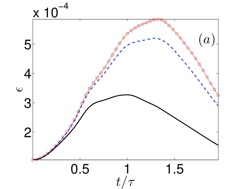
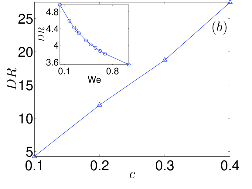
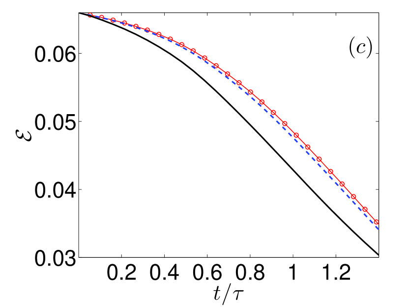
Figure 1: (Color online) (a) Temporal evolution of the energy dissipation rate $\epsilon$ (run NSP-256) for concentrations $c=0.1({{\color[rgb]{0,0,1}--}})$ and $c=0.4($solid line$)$, with $\tau\equiv\sqrt{2{\mathcal{E}}(t=0)/3{\mathbb{L}}^{2}}$; (b) percentage drag-reduction DR versus $c$ (run NSP-192); the inset shows the mild variation in DR with $We$ (runs NSP-96); (c) temporal evolution of the total fluid energy ${\mathcal{E}}$ for concentrations $c=0.1({{\color[rgb]{0,0,1}--}})$ and $c=0.4($solid line$)$ (runs NSP-256). In (a) and (c) the plots for $c=0$ $({\color[rgb]{1,0,0}o-})$ are shown for comparison.

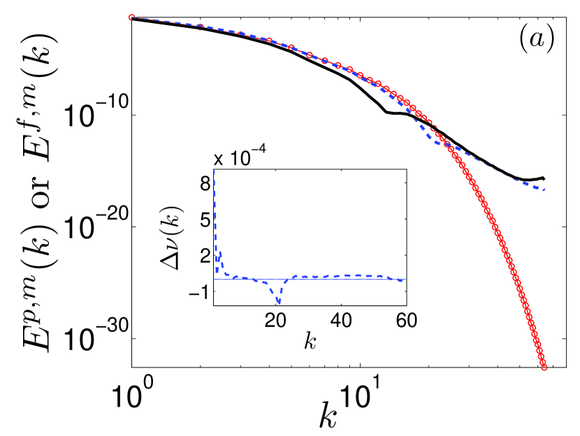
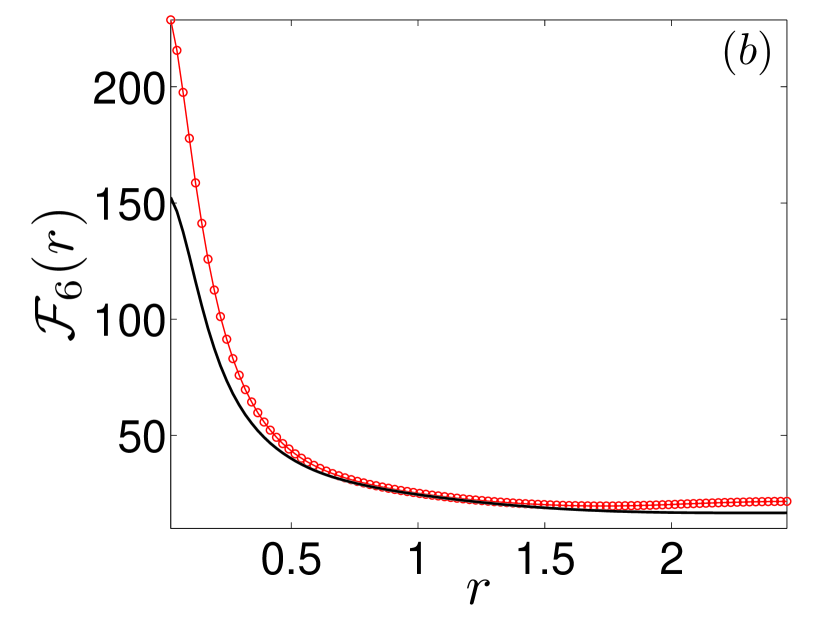
Figure 2: (Color online) (a) Plots of the energy spectra $E^{p,m}(k)$ or $E^{f,m}(k)$ versus $k$ (run NSP-192) for $c=0.1({{\color[rgb]{0,0,1}--}})$ and $c=0.4($solid line$)$ [$E^{p,m}(k)$ is unchanged if we use $N=256$, with all other parameters the same (run NSP-256A)]; inset: polymer contribution to the scale-dependent viscosity $\Delta\nu(k)$ versus $k$ for $c=0.1({\color[rgb]{0,0,1}--})$; $\Delta\nu(k)=0$ $($solid line$)$ is also shown for reference; (b) the hyper-flatness ${\mathcal{F}}_{6}(r)$ as a function of $r$ (run NSP-256) and concentration $c=0.4($solid line$)$. In (a) and (b) the corresponding plots with $c=0$ $({\color[rgb]{1,0,0}o-})$ are shown for comparison. (c) The cumulative PDF $P^{C}(r_{P}^{2}/L^{2})$ versus $r_{P}^{2}/L^{2}$ for $c=0.1({\color[rgb]{0,0,1}--})$ and $c=0.4($solid line$)$ (run NSP-256).

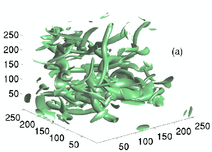
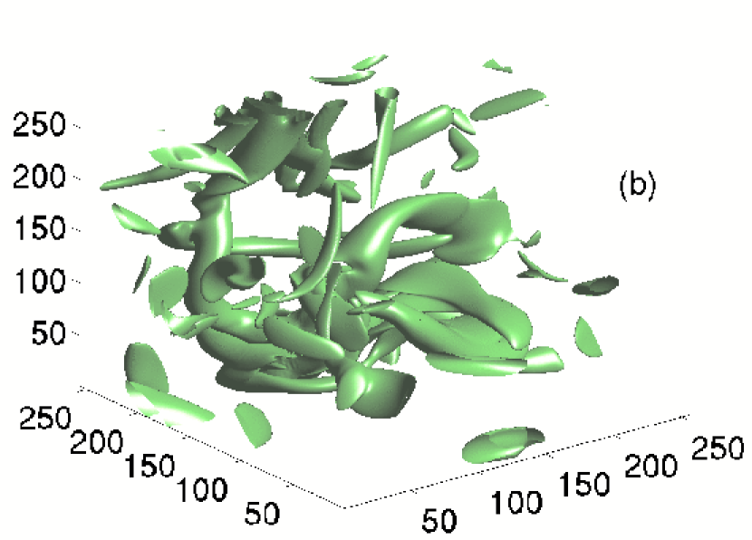
Figure 3: (Color online) Constant-$|\omega|$ isosurfaces for $|\omega|=\langle{|\omega|}\rangle+2\sigma$ at $t_{m}$ without (a) and with (b) polymers, (run NSP-256) and $c=0.4$; $\langle|\omega|\rangle$ is the mean and $\sigma$ the standard deviation of $|\omega|$.

We thank C. Kalelkar, R. Govindarajan, V. Kumar, S. Ramaswamy, L. Collins, and A. Celani for discussions, CSIR, DST, and UGC(India) for financial support, and SERC(IISc) for computational facilities. DM is supported by the Henri Poincaré Postdoctoral Fellowship.

References

- (1) P. Virk, AIChE 21, 625 (1975).
- (2) P. van Dam, G. Wegdam, and J. van der Elsken, J. Non-Newtonian Fluid Mech. 53, 215 (1994).
- (3) J. D. Toonder, M. Hulsen, G. Kuiken, and F. Nieuwstadt, J. Fluid Mech. 337, 193 (1997).
- (4) J. Lumley, J. Polym. Sci 7, 263 (1973).
- (5) K. Sreenivasan and C. White, J. Fluid Mech. 409, 149 (2000).
- (6) P. Ptasinski et al., J. Fluid Mech 490, 251 (2003).
- (7) V. L’vov, A. Pomyalov, I. Procaccia, and V. Tiberkevich, Phys. Rev. Lett. 92, 244503 (2004).
- (8) G. Boffetta, A. Celani, and A. Mazzino, Phys. Rev. E 71, 036307 (2005).
- (9) M. Tabor and P. D. Gennes, Europhys. Lett. 2, 519 (1986).
- (10) J. K. Bhattacharjee and D. Thirumalai, Phys. Rev. Lett. 67, 196 (1991).
- (11) R. Benzi, E. de Angelis, R. Govindarajan, and I. Procaccia, Phys. Rev. E 68, 016308 (2003).
- (12) R. Benzi, E. Ching, and I. Procaccia, Phys. Rev. E 70, 026304 (2004) consider a scale-dependent viscosity for a shell model (but use an artificial diffusivity for polymers for numerical stability).
- (13) C. Kalelkar, R. Govindarajan, and R. Pandit, Phys. Rev. E 72, 017301 (2004).
- (14) E. de Angelis, C. Casicola, R. Benzi, and R. Piva, J. Fluid Mech 531, 1 (2005).
- (15) E. van Doorn, C. White, and K. Sreenivasan, Phys. Fluids 11, 2387 (1999).
- (16) W. McComb, J. Allan, and C. Greated, Phys. Fluids 20, 873 (1977).
- (17) C. Friehe and W. Schwarz, J. Fluid Mech 44, 173 (1970).
- (18) D. Bonn, Y. Couder, P. van Dam, and S. Douady, Phys. Rev. E 47, R28 (1993).
- (19) D. Bonn et al., J. Phys. CM 17, S1219 (2005).
- (20) A. Peterlin, J. Polym. Sci., Polym. Lett. 4, 287 (1966); H. Warner, Ind. Eng. Chem. Fundamentals 11, 379 (1972); R. Armstrong, J. Chem. Phys. 60 724 (1974); E. Hinch, Phys. Fluids 20, S22 (1977).
- (21) J. Hoyt and J. Taylor, Phys. Fluids 20, S253 (1977).
- (22) T. Vaithianathan and L. Collins, J. Comput. Phys. 187, 1 (2003). We correct their Eq.(40) and definition of .
- (23) A. Vincent and M. Meneguzzi, J. Fluid Mech. 225, 1 (1991); C. Canuto, M. Hussaini, A. Quarteroni, and T. Zang, Spectral Methods in Fluid Dynamics (Spinger-Verlag, Berlin, 1988).
- (24) R. Benzi et al., Phys. Rev. E 48, R29 (1993); S. Dhar, A. Sain, and R. Pandit, Phys. Rev. Lett. 78, 2964 (1997).
- (25) Y. Kaneda et al., Phys. Fluids 15, L21 (2003).
- (26) D. Mitra, J. Bec, R. Pandit, and U. Frisch, Phys. Rev. Lett. 94, 194501 (2005).