Examples of Synchronization in Discrete Chaotic Systems

Abstract

This paper presents an application of partial contraction analysis to the study of global synchronization in discrete chaotic systems. Explicit sufficient conditions on the coupling strength of networks of discrete oscillators are derived. Numerical examples and applications to simple systems are presented. Previous researches have shown numerically that the systems under study, when arranged in a network, exhibits rich and complex patterns that can dynamically change in response to variations in the environment. We show how this “adaptation” process strongly depends on the coupling characteristics of the network. Other potential applications of synchronized chaotic oscillators are discussed.

I INTRODUCTION

This paper presents a research focused on coupled discrete dynamical systems [1], [9]. In particular, it is of interest to study the synchronization phenomenon in chaotic systems, i.e. systems in which small differences on the initial conditions can lead to a completely different behaviours in time. In spite of this characteristic, synchronization can be achieved in this type of systems [10], [11]. This work presents a number of examples in which synchronization can be guaranteed by choosing the appropriate coupling strength. The coupling strength can be determinate using partial contraction analysis. This analysis is able to predict complete synchronization independently of the initial conditions, as long as the coupled system verifies certain properties. Besides synchronization, diffusively coupled dynamical systems oscillating chaotically in time have seen to lead to interesting emerging properties due to changes in the environment [$5$]. This feature has been used in this work to simulate the motion of a two–legged robot where each leg is a chaotic oscillator and these oscillators are diffusively coupled. The appeal of such a system is the fast adaptation it shows when sudden unexpected dynamic changes in the environment occur. This method of locomotion does not require any control or optimization process to be performed. Furthermore, this type of analysis can be done on any periodical task that requires fast responses to unpredictable changes.

The role of chaos in “adaptation” and evolution has been widely discussed before [4], [8]. In particular, some research in this area, sometimes known as “adaptation at the edge of chaos”, suggests the possibility that when biological systems adapt in order to survive, the process of evolution may favor those systems that are near a phase transition from order to chaos [8]. In any event, the chaotic behaviour of simple dynamical systems can be exploited to obtain adaptation behaviors to external dynamical disturbances.

The method used is mathematically simple and also similar to for the analysis of coupled dynamical systems [3], [9], [10]. Defining proper matrices to project the states onto the so-called synchronization manifold [10], [11], contraction theory [7], [13], [14], [17] can be used to determine conditions for which a set of coupled identical systems will completely synchronize.

II Mathematical Foundations

As in [$13$], consider a set of coupled dynamical systems and define the vector x{}:

$${{x}}_{\{\}}=\left[\begin{array}[]{c}{x_{1}}\\ {\begin{array}[]{l}{x_{2}}\\ {{\rm\;}\vdots}\\ {x_{n}}\end{array}}\end{array}\right]\Rightarrow\dot{{x}}_{\{\}}=\left[\begin{array}[]{c}{\dot{x}_{1}}\\ {\begin{array}[]{l}{\dot{x}_{2}}\\ {{\rm\;}\vdots}\\ {\dot{x}_{n}}\end{array}}\end{array}\right]$$ (1)

Define the matrices U and V

$$\textbf{U}=\left[\begin{array}[]{cccccc}{1}&{1}&{0}&{0}&{\cdots}&{0}\\ {0}&{1}&{1}&{0}&{\cdots}&{0}\\ {\vdots}&{\vdots}&{\vdots}&{\vdots}&{\cdots}&{\vdots}\\ {1}&{0}&{0}&{0}&{\cdots}&{1}\end{array}\right]$$ (2)

$$\textbf{V}=\left[\begin{array}[]{cccccc}{1}&{-1}&{0}&{0}&{\cdots}&{0}\\ {0}&{1}&{-1}&{0}&{\cdots}&{0}\\ {\vdots}&{\vdots}&{\vdots}&{\vdots}&{\cdots}&{\vdots}\\ {-1}&{0}&{0}&{0}&{\cdots}&{1}\end{array}\right]$$ (3)

such as

$$\begin{array}[]{l}{x^{||}=\textbf{U}x_{\{\}}\Rightarrow\dot{x}^{||}=\textbf{U}\dot{x}_{\{\}}}\\ {x^{\bot}=\textbf{V}x_{\{\}}\Rightarrow\dot{x}^{\bot}=\textbf{V}\dot{x}_{\{\}}}\end{array}$$ (4)

By construction

$$\textbf{UV}^{T}=\left[\begin{array}[]{cccccc}{0}&{1}&{0}&{0}&{\cdots}&{0}\\ {-1}&{0}&{1}&{0}&{\cdots}&{0}\\ {0}&{-1}&{0}&{1}&{\cdots}&{0}\\ {\vdots}&{\vdots}&{\vdots}&{\vdots}&{\cdots}&{\vdots}\\ {0}&{0}&{0}&{-1}&{\cdots}&{1}\\ {0}&{0}&{0}&{\cdots}&{-1}&{0}\end{array}\right]$$ (5)

so $<$ U_i,V_i $>$ = 0, where $<$x,y$>$ denotes standard inner product. Thus, the elements of the vectors $x^{\|}$ and $x^{\bot}$ are orthogonal “one to one”:

$\begin{array}[]{l}{{x}^{||}_{i}=\textbf{U}_{i}{x}_{i}||\textbf{U}_{i}}\\ {{x}^{\bot}_{i}=\textbf{V}_{i}{x}_{i}||\textbf{V}_{i}}\end{array}$ $\rightarrow$ ${x}^{||}_{i}\bot{x}^{\bot}_{i}$

III Contraction Theory for Discrete Systems

Some basic results in Contraction Theory are presented as follows:

Definition 1

Given the systems of equations $x_{i+1}=f_{i}\left(x_{i},i\right)$ , a region of the state space is called contraction region with respect to a uniformly positive definite metric $M_{i}\left(x_{i},i\right)=\theta_{i}^{T}\theta_{i}$ if in that region $[7]$:

$$\exists\beta>0,F_{i}^{T}F_{i}-I\leq-\beta I<0$$ (6)

where

$$F=\theta_{i+1}\frac{\partial f}{\partial x}\theta_{i+1}^{-1}$$ (7)

Theorem 1

Given the systems of equations $x_{i+1}=f_{i}\left(x_{i},i\right)$ , any trajectory, which starts in a ball of constant radius with respect to the metric $M_{i}\left(x_{i},i\right)$, centered about a given trajectory and contained at all times in a contraction region with respect to the metric $M_{i}\left(x_{i},i\right)$, remains in that ball and converges exponentially to this trajectory. Furthermore, global exponential convergence to the given trajectory is guaranteed if the whole state space is a contraction region with respect to the metric $M_{i}\left(x_{i},i\right)$. This corresponds to a necessary and sufficient condition for exponential convergence of the system $[7]$.

Theorem 2

Consider two coupled systems. If the dynamics equations verify

$$x^{\left(A\right)}_{n+1}-h\left(x^{\left(A\right)}_{n}\right)=x^{\left(B\right)}_{n+1}-h\left(x^{\left(B\right)}_{n}\right)$$ (8)

where the function h is contracting, then $x^{(A)}$ and $x^{(B)}$ will converge to each other exponentially, regardless of the initial conditions $[17]$.

Hence, the process of one variable converging exponentially to another, i.e. synchronization, can be seen equivalently as contraction of the projection in the transverse manifold [$13$]. It is clear since the transverse manifold is, by construction, perpendicular to the synchronization manifold:

$$x_{1}\to x_{2}\Leftrightarrow x^{\bot}\to 0$$ (9)

If the projection of a particular solution has null norm in the transverse manifold, it lays entirely on the synchronization manifold (here there are no distinction between synchronization and oscillator dead). Thus, it is only necessary to study the hereafter called error dynamics $x_{i}-x_{j}$, and prove its contracting behaviour. The proof can be seen in $[13]$ and it can be express in rather intuitive terms: synchronization will be achieved if the difference of the states of any two oscillators is zero.

IV Application of Contraction to Chaotic Systems Synchronization

IV-A General Case: Chaotic Maps

In order to study the phenomenon of complete synchronization in chaotic systems, it is usual to work with one-dimensional maps [5], [12] due to the complex behaviours that can be observed from such simple models. When no coupling is present between any of the maps, due to their chaotic nature the systems behave random-like. But when appropriate coupling is build between the maps, one will expect some sort of interaction. Hence, in the case of synchronization or complete synchronization, it is of interest to have a coupling with two main properties [12]:

1. The coupling must make the states of the systems closer to each other, i.e. dissipative coupling.

2. The coupling must not affect the synchronization state.

A general form of this kind of coupling operator of dimension-2 is:

$$L=\left[\begin{array}[]{cc}{1-\alpha}&{\beta}\\ {\beta}&{1-\beta}\end{array}\right]$$ (10)

where 0 $<$ a $<$ 1 and 0 $<$ b $<$ 1. The simplest case of this coupling would be $\alpha$ = $\beta$ = $\varepsilon$ [12]. This case allows the coupling to be symmetric, which leads to a great simplification in the computations needed, and furthermore, it allows the direct application of the proposed method. Hence, it is possible to couple any two maps x and y as [12]:

$$\left[\begin{array}[]{c}{x_{t+1}}\\ {y_{t+1}}\end{array}\right]=\left[\begin{array}[]{cc}{1-\varepsilon}&{\varepsilon}\\ {\varepsilon}&{1-\varepsilon}\end{array}\right]\left[\begin{array}[]{c}{f\left(x_{t}\right)}\\ {f\left(y_{t}\right)}\end{array}\right]$$ (11)

and with a proper choice of the coupling strength $\varepsilon$, the complete synchronization state can be achieved. For example, two oscillators following the well known skew map [8], [12]:

$$f\left(x_{n}\right)=\left\{\begin{array}[]{l}{\frac{x_{n}}{a}{\rm\;\;\;\;if\;\;\;}0\leq x_{n}\leq a}\\ {\frac{\left(1-x_{n}\right)}{\left(1-a\right)}{\rm\;\;if\;\;\;}a\leq x_{n}\leq 1}\end{array}\right.$$

which exhibits pure chaotic behaviour due to the subsequent stretching and folding processes in the interval from 0 to 1 [12]. Two discrete systems of this type, say x and y, can be coupled as in ($11$). Thus, varying the coupling strength $\varepsilon$ it is possible to achieve complete synchronization of the states. The complete proof of this example can be found in [12], where the well known technique of transverse Lyapunov exponents is used [10], [11].

However, theorem 2 from contraction theory provides a simple yet powerful tool to analyze this particular system. The following theorem was presented for the first time in [17]. Using this theorem it is possible to write the system of two skew maps x and y, coupled together in the following form:

$$x_{n+1}-\left(1-2\varepsilon\right)f\left(x_{n}\right)=y_{n+1}-\left(1-2\varepsilon\right)f\left(y_{n}\right)$$ (12)

Hence, it is only necessary to verify that the function

$$h\left(x\right)=\left(1-2\varepsilon\right)f\left(x\right)$$ (13)

is contracting for f(x) in ($12$) (for a particular metric). As $\partial$f(x)/$\partial$x is not continuous, two cases must be taken into account. Each one of these cases should give an interval for e in which contraction of the function h(x) is guaranteed. The general result is the intersection of these two intervals (in fact, the supremum or the biggest set contained in the intersection of the intervals obtained). In this particular example, we must show that the Jacobian

$$F=\frac{\partial h\left(x\right)}{\partial x}=\left(1-2\varepsilon\right)\frac{\partial f\left(x\right)}{\partial x}$$ (14)

is contracting in some metric M. Indeed, if M is equal the identity matrix I, for the two cases we find the suitable intervals

$$\begin{array}[]{l}{0\leq x\leq a{\rm\;\;\;}\to{\rm\;\;}\frac{\partial f\left(x\right)}{\partial x}={\rm\;\;\;}\frac{1}{a}{\rm\;\;\;\;;\;\;\;}{\rm\;\;\;\;}\frac{a-1}{2}<{\rm\;\;}\varepsilon{\rm\;\;}<\frac{a+1}{2}}\\ \\ {a\leq x\leq 1{\rm\;\;\;}\to{\rm\;\;}\frac{\partial f\left(x\right)}{\partial x}=\frac{1}{a-1}{\rm\;\;;\;\;}{\rm\;\;\;\;\;\;\;}\frac{a}{2}{\rm\;\;\;}<{\rm\;\;}\varepsilon{\rm\;\;}<1-\frac{a}{2}}\end{array}$$

Thus, the supremum of the intersection of the two intervals is the second one (as it is contained in the first interval). It is straight forward to verify that the use of the transverse manifold leads to the exactly same conditions as before, i.e. an interval for $\varepsilon$ in which the error dynamics is contracting in the same metric as before. In fact, the two synchronization intervals obtained for the error are

$$\begin{array}[]{l}{0\leq x\leq a{\rm\;\;\;}\to{\rm\;\;}e{}_{n+1}=\frac{\left(1-2\varepsilon\right)}{a}e{\rm\;\;;\;\;}\frac{a-1}{2}<{\rm\;\;}\varepsilon{\rm\;\;}<\frac{a+1}{2}}\\ \\ {a\leq x\leq 1{\rm\;\;\;}\to{\rm\;\;}e{}_{n+1}=\frac{\left(1-2\varepsilon\right)}{a-1}e{\rm\;\;\;;\;\;}\frac{a}{2}{\rm\;\;\;}<{\rm\;\;}\varepsilon{\rm\;\;}<1-\frac{a}{2}}\end{array}$$

Going beyond the analysis done by transverse Lyapunov exponents, the contraction theory is capable of giving intervals where the selected coupling strength $\varepsilon$ guarantees complete synchronization. This can be clearly seen in figure 1. For two coupled oscillators X and Y and a = 0.7, the proposed method predicts complete synchronization (in which the values lie on the X = Y line) for a coupling strength between 0.35 and 0.65. Fig. 1 shows two cases.

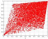
Figure 1: Chaotic oscillators coupled with different strengths. Left: e = 0.9, i.e. outside of the contraction range. Right: e = 0.4, i.e inside the predicted synchronization interval.

IV-B Coupled Map Lattice (CML)

In [5], the authors proposed a more general model a coupling in which the states takes into account the dynamics of any other oscillator “next to it” equally weighted:

$$x^{i}_{n+1}=\left(1-\varepsilon\right)f\left(x^{i}_{n}\right)+\frac{\varepsilon}{2}\left(f\left(x^{i+1}_{n}\right)+f\left(x^{i-1}_{n}\right)\right)$$ (15)

As it can be seen, at the iteration n+1 the dynamics of the i-th oscillator depends on its previous state (weighted by 1-$\varepsilon$) and the previous state of the “nearest” two oscillators, e.g. (i-1)-th oscillator and the (i+1)-th oscillator, equally weighted by a factor of $\varepsilon$ /2. Let $x_{n+1}$= f(x) =1 – a$x_{n}^{2}$ where a is a positive constant and write the system in the following form:

$$x^{i}_{n+1}=f\left(x^{i}_{n}\right)+\frac{\varepsilon}{2}\left(f\left(x^{i+1}_{n}\right)+f\left(x^{i-1}_{n}\right)-2f\left(x^{i}_{n}\right)\right)$$ (16)

Thus, for two coupled oscillators x and y, the matrices U and V are vectors

$$\begin{array}[]{l}{\textbf{U}=\left[\begin{array}[]{cc}{1}&{1}\end{array}\right]}\\ {\textbf{V}=\left[\begin{array}[]{cc}{1}&{-1}\end{array}\right]}\end{array}$$

and the dynamics of the projection on the synchronization manifold $x^{\bot}$ = e = x - y is given by

$$e_{n+1}=x_{n+1}-y_{n+1}=\left(\frac{3\varepsilon}{2}-1\right)a\sigma e_{n}$$ (17)

where $\sigma$ = x+y, and no approximations, e.g. linearization about a certain point, have been made. Now, a virtual auxiliary system can be constructed [17]

$$w_{n+1}=f\left(w_{n}\right)=\left(\frac{3\varepsilon}{2}-1\right)a\sigma w_{n}$$ (18)

where both 0 and $e_{n}$ are particular solutions. This new map shall be contracting, i.e. $\partial$f($w_{n}$)/$\partial$$w_{n}$ is u.n.d , in any case for an identity metric, i.e. in ($7$) the matrix M = I (identity matrix), and therefore e will tend exponentially to 0 if [7]:

$$\frac{2\left(a-\frac{1}{\sigma}\right)}{3a}<\varepsilon<\frac{2\left(a+\frac{1}{\sigma}\right)}{3a}$$ (19)

Letting $\sigma$ to be variable, ($19$) describes a family of hyperbolas in the a - $\varepsilon$ plane. Now, it is necessary to find a region in the a - $\varepsilon$ plane that guarantees contraction, i.e. a region where any pair (a - $\varepsilon$) will assure contraction of the system. This can be easily done by finding the supremum of the areas defined between the curves of the hyperbolas. In Fig. 2 some of the hyperbolas are shown for a = 1.7, where the map exhibits a chaotic behaviour ($\sigma_{1}$ $<$ $\sigma_{2}$ $<$ $\sigma_{3}$).

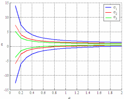
Figure 2: Family of hyperbolas defining contraction regions for the coupled system. The hyperbola with the “narrowest” area between the curves ($\sigma_{3}$) defines the sufficient contraction region for the error dynamics

In this particular case, it is found that the supremum is given by the area between the curves o the hyperbola with $\sigma$ =2(2/$\sqrt{a}$). Now, since the initial value of x is random number between 0 and 1, the absolute values of x and y are always less than ($\sqrt{2/a}$) $\approx$ 1 (for values of a which guarantee chaotic behaviour), it can be easily shown that:

$${-1<1-ax^{2}<1}\\ \Rightarrow{-2<-ax^{2}<0}$$ (20)

Since both a and $x^{2}$ are always positive, the condition in ($20$) is true.

The values of a which guarantee chaotic behaviour can be found by computing the Lyapunov exponents of the map as a varies [16]. The first Lyapunov exponent for different values of a is shown in Fig. 3.

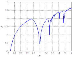
Figure 3: First Lyapunov exponent of the logistic map as a varies

It can be seen that the values close to 2 guarantee chaotic behaviour. Hence, the limit, i.e. the narrowest hyperbola is given by $\sigma\approx 2$ , since

$$\frac{2a-1}{3a}<\varepsilon<\frac{2a+1}{3a}$$ (21)

It is worth noticing that this is the same result on would find applying theorem $2$: writing the system of equations in the form:

$$x_{n+1}-\left(\frac{3\varepsilon}{2}-1\right)ax_{n}^{2}=y_{n+1}-\left(\frac{3\varepsilon}{2}-1\right)ay_{n}^{2}$$ (22)

where, in order to assure synchronization of the states, the function:

$$h\left(x\right)=\left(\frac{3\varepsilon}{2}-1\right)ax^{2}$$ (23)

must be contracting in some metric. Using the identity metric the same results as before are found.

Thus, the expected behaviour should be (looking for positive values of $\varepsilon$ ) as presented in figure 4, where the shaded area represents the guaranteed contraction region for the coupled system (recall that each oscillator without coupling follows its own nominal chaotic dynamics):

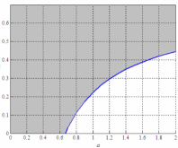
Figure 4: The shaded area is the guaranteed contraction region for $\sigma$= 2 and an identity metric

Numerical experiments were performed: using a Sobolev distribution (which gives a random but uniformly distributed cloud of points in a determined region) in the a-$\varepsilon$ plane, Fig. 4 shows the norm of the error vector for each couple (a,$\varepsilon$) after a transient time of 300 iterations. We find indeed, as shown in figure 5, that the actual region of guaranteed contraction for the coupled system resembles the one predicted by the proposed method.

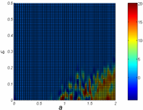
Figure 5: Actual contraction region for $\sigma$ = 2. The dark area represents a set of pairs (a,$\varepsilon$ ) for which the norm of the error is zero after the transient

V Simulations on the Coupled Map Lattice

Using the previous results, the coupling strength can be tuned to guaranteed synchronization, as shown in Fig. 6.

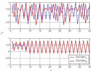
Figure 6: Two chaotic discrete oscillators. Above: non coupled. Below: properly coupled

From these results, it is clear how, using a value for the coupling strength that satisfy the conditions for the contracting error dynamics in the synchronization manifold, the two systems will tend exponentially to each other (equivalently, the error will tend exponentially to the origin of the synchronization manifold).

VI Adaptation and Emerging Behaviour Via Sensing

Let’s modify the coupled map lattice considered above such as the system receives information of the environment via sensing. The signal coming from the sensors can be any kind of signal (rotation angle, voltage, etc) as long as it can be related somehow to the state variable x. Let’s consider for example the following dynamics as proposed in [5]:

$$x^{i}_{n+1}=f\left(x^{i}_{n}+\varepsilon_{1}\left(\bar{s}_{n}-s^{i}_{n}\right)+\varepsilon_{2}\left(\frac{s^{i+1}_{n}+s^{i-1}_{n}}{2}-s^{i}_{n}\right)\right)$$ (24)

where $s^{i}_{n}$ denotes the sensor reading at the iteration n and $\bar{s}_{n}$ is the mean value of the sensors at the iteration n. The meaning of this type of coupling is as follows: each oscillator follows its own the chaotic dynamics, but this is “adjusted and updated” to reduce the global (via $\varepsilon_{1}$) and local (via $\varepsilon_{2}$) difference in the sensors [5]. Fig. 7 shows the model schematically.

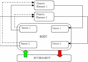
Figure 7: Outline of the model. This model is inspired on the one proposed in [5]

Let’s suppose that each oscillator represents the dynamics of a motor and that each motor is driving a leg of a simple two–legged robot. Thus, each leg has an actuator following the proposed dynamics coupled in order to achieve synchronization. Let the variable x be the command to the actuator (torque $\tau$) and the signal sensed (s) be the angle $\theta$. This to variables are related as follows in Fig. 8:

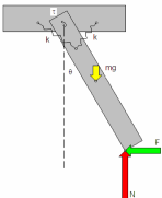
Figure 8: Model used for the two–legged robot simulation

Following the method as done previously in (18), the error dynamics is given by:

$$e_{n+1}=-a\sigma e_{n}+2a\left(\frac{\varepsilon_{1}}{2}+\varepsilon_{2}\right)\sigma(s_{n}^{(A)}-s_{n}^{(B)})$$ (25)

For this is particular case, the angle s can be related directly to the torque x in a linear fashion, e.g. in ($25$)
s = mx + b (where the constants m and b are given by the sensor characteristics). Hence once again, a virtual auxiliary system can be construct

$$y_{n+1}=f\left(y_{n}\right)=-a\sigma y_{n}+2a\left(\frac{\varepsilon_{1}}{2}+\varepsilon_{2}\right)\sigma(s_{n}^{(A)}-s_{n}^{(B)})$$

where 0 and $e_{n}$ are particular solutions. Using an identity metric M = I, the system shall be contracting, i.e. the error e will converge exponentially to 0, for:

$$\begin{array}[]{l}{\frac{\psi(a-\frac{1}{\sigma})}{2a}<\frac{\varepsilon_{1}}{2}+\varepsilon_{2}<\frac{\psi(a+\frac{1}{\sigma})}{2a}{\rm\;\;\;\;\;\;\;}}\vskip 12.0pt plus 4.0pt minus 4.0pt\\ {where{\rm\;\;\;\;\;\;\;\;}\psi=\left(K^{*}-Nl+mg\frac{l}{2}\right)}\end{array}$$ (26)

and $K^{*}$ is the equivalent stiffness of the two springs. Fig. 9 shows two coupled oscillators starting at random initial conditions. The complete synchronization is achieved by tuning the coupling strength to be inside the predicted synchronization range.

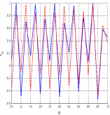
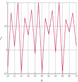
Figure 9: Proper selection of the coupling strength assures complete synchronization. Left: coupling strength outside the contraction range. Right: coupling strength inside the contraction range

VII Why Bother with Chaotic Systems?

At this point it seems natural to ask why it is worth working in a chaotic regime, since similar results, specifically synchronization, can be achieved with non chaotic oscillators. Apparently the key to answer this questions is adaptability. The following example shows the advantages of a chaotic regime. Assume the two–legged robot under three different conditions: first assume that the legs are chaotic but not coupled; second, the legs are coupled but not chaotic; and finally the legs are coupled working in the chaotic regime. As an external condition assume that the left leg senses a decrease of 25% in the friction coefficient after y = 1 m. Figure 10 shows the results obtained by simulation.

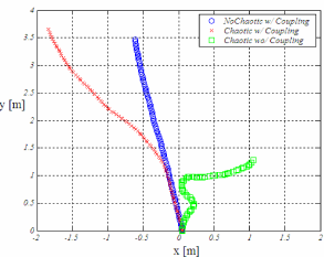
Figure 10: Trajectory followed by the robot in the x–y plane

Apparently, the condition coupled–chaotic is more sensitive to external changes in the environment, which can be seen as an emerging adaptive property of the system.

Another simulation under the condition coupled–chaotic was done in which after some fixed traveling distance one of the legs “feels” a change in the surface, e.g. in this case the sensor detects a change in the angle due to a decrease in the friction coefficient between the leg and the surface. The results suggest that the change in the behaviour depends on the magnitude of the change in the environment.

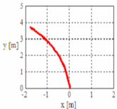
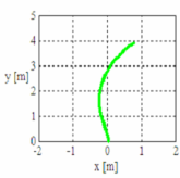
Figure 11: Friction coefficient between leg and surface decrease after y = 1. Left: decrease of 25% in the friction coefficient in the left leg. Right: decrease of 40% in the friction coefficient in the right leg

These results suggest that the idea of adaptation to changes in the environment is intrinsic to the system dynamics. In the sense of adaptation and evolution [$5$] and perhaps abusing of the terminology, chaotic oscillations may be regarded as “mutants” from a nominal (non chaotic) oscillation pattern. Such deviations from the smooth nominal behaviour give the system the capacity of response faster to external inputs. Furthermore, due to the nature of chaotic oscillations, e.g. strange attractors where the trajectories are random–like yet confined in space [15], they appear to be a good compromise between a “mutation” sufficiently strong to make the system adapt to a new external condition but mild enough to maintain information from the previous behaviour.

Finally, note that the analysis does not require any goal direction, because the system, due to its simple configuration, tends to “walk straight ahead”. This feature makes unnecessary the implementation of any mean of command, e.g. algorithms deciding to freeze a leg at a certain moment. The system simply moves forward, responding quickly to changes in the environment and, more interesting, this response is proportional to the magnitude of the change.

But the reason why the chaotic regime exhibits this adaptive behaviour remains an open question. In order to understand this phenomenon let’s take the following example: assume that each movement of the legs takes place in 1 second (arbitrary time interval where one oscillation takes place). It is obvious that the power spectral density of the signal (PSD) will have, in any case, a peak at 0.5 Hz (it takes 2 seconds for the leg to complete a cycle forward-backward).

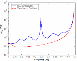
Figure 12: Power spectral density of a chaotic and a non-chaotic oscillator

Fig. 12 shows the mean PSD of 128 runs starting at random initial conditions: the mean of 128 non chaotic signals, i.e. with a value of a that makes the first Lyapunov exponent negative, e.g. a = 1.1 (dashed line) and the mean of 128 chaotic signals, i.e. a = 1.7 (solid line). Both signals are subjected to a equivalent coupling strength

It can be seen how the chaotic signal carries energy at some other different frequencies than the trivial one. In particular, it can be seen that the period-doubling phenomenon occurs (peak at half the main frequency). Due to its chaotic nature, this particular feature allows the system to have richer movement patterns in changing environments (because different frequencies are being excited by the same signal).

For example, consider the case of a small vehicle where each wheel is driven by a chaotic oscillator and these oscillators are coupled as before. As any road profile irregularity can be describe as an ergodic random process in space [2], a vehicle traveling at constant speed V (in average) will sense an input which is an ergodic random process in time. As the energy of the signal in chaotic regime is amplified at more particular frequencies, the natural response of the system, e.g. the legged robot or the wheeled vehicle, will show richer outputs. This could be seen as an advantage when dealing with challenging and changing environments.

VIII Networks of Symmetric Coupled Oscillators

Up to this point, this work has focused on two coupled oscillators. However, the extension to more oscillators in a symmetric network is straight forward. Indeed, as it will be shown in this section, the synchronization analysis of this particular type of networks can be done as if it were composed by two oscillators.

Let’s start by saying that matrices U and V in ($2$) and ($3$) can always be defined for n identical oscillators with scalar dynamics and symmetric coupling, leading to a synchronization of the states of any two adjacent oscillators.

Now, suppose n identical oscillators, coupled in such way that the each oscillator updates its own dynamics by sensing the dynamics of every other oscillator in the network. Furthermore, suppose that the magnitude of the coupling strength is equal for any pair of oscillators in the network. The structure of a network with verifying such conditions is known as “all–to–all” symmetry structure [17]. As a general case, consider the Coupled Map Lattice:

$$\left[\begin{array}[]{c}{x^{\left(1\right)}_{t+1}}\\ {x^{\left(2\right)}_{t+1}}\\ {\vdots}\\ {x^{\left(n\right)}_{t+1}}\end{array}\right]=\left[\begin{array}[]{cccc}{1-\varepsilon}&{g\left(\varepsilon\right)}&{\cdots}&{g\left(\varepsilon\right)}\\ {g\left(\varepsilon\right)}&{1-\varepsilon}&{\cdots}&{g\left(\varepsilon\right)}\\ {\vdots}&{\vdots}&{\ddots}&{\vdots}\\ {g\left(\varepsilon\right)}&{g\left(\varepsilon\right)}&{\cdots}&{1-\varepsilon}\end{array}\right]\left[\begin{array}[]{c}{f\left(x^{\left(1\right)}_{t}\right)}\\ {f\left(x^{\left(2\right)}_{t}\right)}\\ {\vdots}\\ {f\left(x^{\left(n\right)}_{t}\right)}\end{array}\right]$$ (27)

where f($x_{t}^{(k)}$) is any function representing a discrete dynamical system (for k = 1, 2,…, n) and g($\varepsilon$) is a general function of the coupling strength. Using (4), it is possible to find the projection of the system on the transverse manifold, leading to a (n – 1) dynamics of the form

$$e_{n+1}=\Upsilon e_{n}$$ (28)

where $\Upsilon$ is a diagonal matrix where the diagonal elements are functions of the form $\upsilon_{jj}$($\varepsilon$, $x_{t}^{(j)}$ , $x_{t}^{(j+1)})$ for j = 1, 2,…, n–1. Thus, each element of the diagonal is a function that can be expressed for any pair of oscillators in a “two-by-two” fashion. If $\upsilon_{jj}$ is upper bounded, then the coupling strength $\varepsilon$ can always be tuned to guaranteed uniformly negative definiteness of the diagonal matrix $\Upsilon$ [$17$]. It is worth noticing that in the case of chaotic oscillators the condition on the upper bounded of the function is guaranteed by the strange attractor behaviour [$16$], as agreed in section VIII.

This results leads to a convenient simplification in the analysis of any symmetric network of oscillators, since it is necessary to study one single function g to guarantee complete synchronization. Furthermore, it can be stated that the synchronization analysis of any network of oscillators with an “all–to–all” symmetry structure can be made studying the uniformly negative definiteness of a single scalar function. For example, for three discrete oscillators x, y and z:

$$\begin{array}[]{l}{x_{n+1}=f\left(x\right)=1-ax_{n}^{2}}\\ {y_{n+1}=f\left(y\right)=1-ay_{n}^{2}}\\ {z_{n+1}=f\left(z\right)=1-az_{n}^{2}}\end{array}$$ (29)

working in chaotic regime, e.g. a = 1.7, coupled by a linear operator in the form

$$\left[\begin{array}[]{c}{x_{t+1}}\\ {\begin{array}[]{l}{y_{t+1}}\\ {z_{t+1}}\end{array}}\end{array}\right]=\left[\begin{array}[]{ccc}{1-\varepsilon}&{\frac{\varepsilon}{2}}&{\frac{\varepsilon}{2}}\\ {\frac{\varepsilon}{2}}&{1-\varepsilon}&{\frac{\varepsilon}{2}}\\ {\frac{\varepsilon}{2}}&{\frac{\varepsilon}{2}}&{1-\varepsilon}\end{array}\right]\left[\begin{array}[]{c}{f\left(x_{t}\right)}\\ {\begin{array}[]{l}{f\left(y_{t}\right)}\\ {f\left(z_{t}\right)}\end{array}}\end{array}\right]$$ (30)

can be analyzed as previously, e.g. $x_{1}^{\bot}$ = $e^{(1)}$ = x – y and $x_{2}^{\bot}$ =$e^{(2)}$ = y – z leading to

$$\left[\begin{array}[]{l}{e^{\left(1\right)}_{n+1}}\\ {e^{\left(2\right)}_{n+1}}\end{array}\right]=\left[\begin{array}[]{cc}{\left(\varepsilon-1\right)a\sigma_{1}}&{0}\\ {0}&{\left(\varepsilon-1\right)a\sigma_{2}}\end{array}\right]\left[\begin{array}[]{l}{e^{\left(1\right)}_{n}}\\ {e^{\left(2\right)}_{n}}\end{array}\right]=Fe_{n}$$ (31)

where $\sigma_{1}$ = (x + y) and $\sigma_{2}$ = (y + z). Once again, a virtual auxiliary system in the form

$$\left[\begin{array}[]{l}{p_{n+1}}\\ {q_{n+1}}\end{array}\right]=\left[\begin{array}[]{cc}{\left(\varepsilon-1\right)a\sigma_{1}}&{0}\\ {0}&{\left(\varepsilon-1\right)a\sigma_{2}}\end{array}\right]\left[\begin{array}[]{l}{p_{n}}\\ {q_{n}}\end{array}\right]=F\left[\begin{array}[]{l}{p_{n}}\\ {q_{n}}\end{array}\right]$$ (32)

for which the vectors 0 and $e_{n}$ are particular solutions. Thus, the states will converge exponentially to each other for a coupling strength $\varepsilon$ that guarantees uniformly negative definiteness of the matrix F, i.e. the largest singular value of F remains smaller than 1 uniformly [3]. This is easily done (due to the diagonal form of the matrix F) by tuning the parameter $\varepsilon$ in the function

$$\gamma\left(\varepsilon\right)=\left(\varepsilon-1\right)\sigma_{k}a$$ (33)

so that $\gamma$ is uniformly negative definite. The upper bounded value of $\sigma_{k}$ is easily checked from the previous examples ($\sigma_{k}\approx 2$).

Finally, for more general systems, the system of equations in (29) can always be expressed in such way that the following theorem from classical contraction analysis can be directly applied [17].

Theorem 3

Consider q coupled systems. IF a contracting function h($x_{i}$) exists such that

$$x^{\left(1\right)}_{n+1}-h\left(x^{\left(1\right)}_{n}\right)=x^{\left(2\right)}_{n+1}-h\left(x^{\left(2\right)}_{n}\right)=...=x^{\left(q\right)}_{n+1}-h\left(x^{\left(q\right)}_{n}\right)$$

THEN all the systems synchronize exponentially, regardless of the initial conditions.

In the case of the last example, the system dynamics can be expressed as

$$x_{t+1}-\left(\varepsilon-1\right)ax^{2}_{t}=y_{t+1}-\left(\varepsilon-1\right)ay^{2}_{t}=z_{t+1}-\left(\varepsilon-1\right)az^{2}_{t}$$ (34)

for which the analysis of the function h($x_{t}$) = ($\varepsilon$ – 1)$ax_{t}^{2}$ and the tuning of $\varepsilon$ to achieve uniformly negative definiteness of h, leads to the same result as above.

IX CONCLUSIONS AND FUTURE WORKS

IX-A Conclusions

This paper has shown the feasibility of studying synchronized discrete chaotic oscillators, by means of a differential analysis of the nonlinear system. Different kinds of networks and coupling operators can be analyzed globally by simple method. Further investigations on the emerging adaptation properties of such systems are necessary for practical implementations.

IX-B Future Works

Future work will be focus on the extension to systems with more degrees of freedom. Some of the work done on synchronization is intended to be implemented in a set of Lego Mindstorm${}^{\hbox to0.0pt{$\bigcirc$\hss}\scriptstyle\,\,\rm R\;}$ . A small two-wheel vehicle was built using the set of Lego${}^{\hbox to0.0pt{$\bigcirc$\hss}\scriptstyle\,\,\rm R\;}$ blocks and the input signal to the two motors driving the wheels is given by ($26$). The algorithm is intended to be implemented using the angle of rotation as the sensed signal, i.e in accordance with the model of the two-legged robot presented in simulations.

X ACKNOWLEDGMENTS

Juan C. Botero thanks Prof. G. Mastinu and Prof. M. Gobbi for their support and the NSL staff at MIT for their constant help.

References

- [1] P. Ashwin. “Synchronization from Chaos”. Nature 422, 2003, pp. 384 - 385.
- [2] M. Gobbi and G. Mastinu. “Analytical Description and Optimisation of the Dynamic Behaviour of Passively Suspended Road Vehicles”. Journal of Sound and Vibration, 245 (3), 2001, pp. 457 - 481.
- [3] E.M. Izhikevich. Dynamical Systems in Neuroscience: The Geometry of Excitability and Bursting. The MIT Press. Cambridge. 2007.
- [4] S. Kauffman. “Requirements for evolvability in complex systems: Orderly dynamics and frozen components”. Physica D 42, 1990, pp. 135 - 152.
- [5] Y. Kuniyoshi and S.Suzuki. “Dynamic Emergence and Adaptation Behavior Through Embodiment as Coupled Chaotic Field”. Proceedings of 2004 IEEE/RSJ International Conference on Intelligent Robots and Systems. Sendai, Japan. 2004.
- [6] S.A.Levin. “Complex Adaptive Systems: Exploring the known, the unknown and the unknowable”. Bulletin of the American Mathematical Society 40 (1), 2002. pp. 3 - 19.
- [7] W. Lohmiller and J.J.E. Slotine. “On Contraction Analysis for Nonlinear Systems” Automatica 34 (6), 1998.
- [8] M. Mitchell, J. Hraber and P. Crutchfield. “Revisiting the Edge of Chaos: Evolving Cellular Automata to Perform Computations”. Santa Fe Institute. 1993. Santa Fe Institute Working Paper # 93–03–014.
- [9] H. Nijmeijer. “A dynamical control view on synchronization” Physica D 154, 2001. pp. 219 - 228.
- [10] L.M. Pecora, T.L. Carroll, G. Johnson, D.J. Mar and J.F Heagy. “Fundamentals of Synchronization in Chaotic Systems, Concepts and Applcations”. Chaos 7 (4), 1997.
- [11] L.M. Pecora and T.L. Carroll. “Driving Systems with Chaotic Signals”. Physical Review A 44 (4), 1991.
- [12] A.S. Pikovsky, M.G. Rosenblum and J. Kurths, ed. Synchronization. A Universal Concept in Nonlinear Sciences. Cambridge University Press. 2001.
- [13] Q. Pham and J.J.E. Slotine. “Stable Concurrent Synchronization in Dynamics System Networks”. MIT-NSL Report, 2005.
- [14] J.J.E. Slotine. “Modular Stability Tools for Distributed Computation and Control”. Int. J. Adaptive Control and Signal Processing, 17(6), 2003.
- [15] E. Solak. “A reduced-order observer for the synchronization of Lorenz systems”. Physycs Letters A 325, 2004. pp. 276 - 278.
- [16] S. Strogatz. Nonlinear Dynamics and Chaos: with Applications to Physics, Biology, Chemistry and Engineering. Addison Wesley Publ. 1994.
- [17] W. Wang and J.J.E. Slotine. “On Partial Contraction Analysis for Coupled Nonlinear Oscillators”. Biological Cybernetics, 92 (1), 2004.