[Phys. Rev. Lett. 99, 014101 (2007)]

Leading Pollicott-Ruelle Resonances and Transport in Area-Preserving Maps

Abstract

The leading Pollicott-Ruelle resonance is calculated analytically for a general class of two-dimensional area-preserving maps. Its wave number dependence determines the normal transport coefficients. In particular, a general exact formula for the diffusion coefficient $D$ is derived without any high stochasticity approximation and a new effect emerges: The angular evolution can induce fast or slow modes of diffusion even in the high stochasticity regime. The behavior of $D$ is examined for three particular cases: (i) the standard map, (ii) a sawtooth map, and (iii) a Harper map as an example of a map with nonlinear rotation number. Numerical simulations support this formula.

Diffusion is a paradigm of deterministic chaos and its study is not new, dating back to Chirikov Chirikov . Its existence in Hamiltonian systems has been extensively established using a variety of approaches Rechester ; Abarbanel ; Cary ; McKay ; Dana ; Hatori . However, it was not clear that a satisfactory transport theory could be properly formulated. In order to understand deterministic diffusion, nonequilibrium statistical mechanics was suitably combined with dynamical system theory Gaspard ; Dorfman . In this modern formulation, the stochastic properties of chaotic systems can be determined by the spectral properties of the Perron-Frobenius operator $U$. One of the most important properties is the exponential relaxation to the thermodynamic equilibrium, explained in great detail at the microscopic level. The relaxation rates $\gamma_{m}$, known as Pollicott-Ruelle (PR) resonances Pollicott ; Ruelle , are related to the poles $z_{m}$ of the matrix elements of the resolvent $R(z)=(z-U)^{-1}$ as $z_{m}=e^{\,\gamma_{m}}$. These resonances are located inside the unit circle in the complex $z$ plane, whereas the spectrum of $U$ is confined to the unit circle because of unitarity Hasegawa2 . Furthermore, the wave number dependence of the leading PR resonance determines the normal diffusion coefficient for spatially periodic systems Cvitanovic ; Tasaki . These results are rigorous only for hyperbolic systems, though they have been confirmed in the high stochasticity approximation for some mixed systems such as the kicked rotor (standard map) Khodas , the kicked top Weber and the perturbed cat map Blum . The PR resonances are essential not only in classical dynamics but also in quantum dynamics. Recently, a microwave billiard experiment demonstrated a deep connection between quantum properties and classical diffusion through the spectral autocorrelation function Pance .

In this Letter, the leading PR resonance will be calculated analytically for the general class of two-dimensional area-preserving maps

$$\begin{array}[]{l}I_{n+1}=I_{n}+K\,f(\theta_{n})\,,\\ \theta_{n+1}=\theta_{n}+c\,\alpha(I_{n+1})\qquad\mbox{mod}\,2\pi,\end{array}$$ (3)

defined on the cylinder $-\pi\leq\theta<\pi$, $-\infty<I<\infty$. Here $f(\theta)$ is the impulse function, $\alpha(I)=\alpha(I+2\pi r)$ is the rotation number, $c$ and $r$ are real parameters, and $K$ is the stochasticity parameter. This map is commonly called the radial twist map Lichtenberg periodic in action (the nonperiodic case can be considered in the limit $r\rightarrow\infty$). Although considerable theoretical development in the study of diffusion has been achieved for the linear rotation number (LRN) case $c\,\alpha(I)\equiv I$ Rechester ; Abarbanel ; Cary ; McKay ; Dana , many physically realistic systems are best described just by the nonlinear cases. Such maps have been extensively used in various areas of physics, especially in celestial mechanics celestial , plasma and fluid physics plasma , and astrophysics and accelerator devices accelerator ; Lichtenberg . However, the normal transport properties of such maps have not been studied previously Hatori .

The analysis of the map (3) is best carried out in Fourier space. The Fourier expansion of distribution function at the $n$th time, denoted by $\rho_{n}$, is given by

$$\rho_{n}(I,\theta)=\sum_{m}\int dq\,e^{i(m\theta+qI)}a_{n}(m,q)\,.$$ (4)

The moments can be found from the Fourier amplitudes via $\langle I^{\,p}\rangle_{n}=(2\pi)^{2}\,[(i\,\partial_{q})^{p}\,a_{n}(q)]_{q=0}$, where $a_{n}(q)\equiv a_{n}(0,q)$. The discrete time evolution of the probability density $\rho$ is governed by the Perron-Frobenius operator $U$ defined by $\rho_{n+1}(I,\theta)=U\rho_{n}(I,\theta)$. The matrix representation of $U$ may be considered as the conditional probability density for the transition of the initial state $(I^{\prime},\theta^{\prime})$ to a final state $(I,\theta)$ in a one time step, ruled by (3). The law of evolution of the Fourier coefficients will be given by

$$a_{n}(m,q)=\sum_{m^{\prime}}\int dq^{\prime}\,\mathcal{A}_{m}(r,c,q^{\prime}-q)\,\mathcal{J}_{m-m^{\prime}}(-Kq^{\prime})\,a_{n-1}(m^{\prime},q^{\prime})\,,$$ (5)

where $a_{0}(m,q)=(2\pi)^{-2}\exp[-i(m\theta_{0}+qI_{0})]$. The Fourier decompositions of the $\alpha(I)$ and $f(\theta)$ functions are

$$\mathcal{A}_{m}(r,c,x) = \sum_{l}\delta(lr^{-1}-x)\,\mathcal{G}_{l}(r,mc)\,,$$ (6)

$$\mathcal{G}_{l}(r,x) = \frac{1}{2\pi}\int d\theta\,\exp\{-i[x\alpha(r\theta)-l\theta]\}\,,$$ (7)

$$\mathcal{J}_{m}(x) = \frac{1}{2\pi}\int\,d\theta\,\exp\{-i[m\theta-xf(\theta)]\}\,.$$ (8)

If the rotation number $\alpha(I)$ is an odd function, then $\mathcal{G}_{l}(r,x)$ is a real function and $\mathcal{G}_{\pm|l|}(r,x)=\mathcal{G}_{\left|l\right|}(r,\pm\,x)$. The integral function $\mathcal{J}_{m}(x)$ assumes the following series expansions $\mathcal{J}_{m}(x)=\delta_{m,0}+\sum_{n=1}^{\infty}c_{m,n}\,x^{n}$, whose coefficients are given by

$$c_{m,n}=\frac{1}{2\pi}\frac{i^{n}}{n!}\int\,d\theta\,f^{n}(\theta)\,e^{-im\theta}\,.$$ (9)

Note that, if $f(-\theta)=-f(\theta)$, the coefficients $c_{m,n}$ are real for all $\left\{m,n\right\}$ and $\mathcal{J}_{-m}(x)=\mathcal{J}_{m}(-x)$.

Let us consider the decomposition method of the resolvent $R(z)$ based on the projection operator techniques utilized in Hasegawa1 . The law of evolution $(\ref{evolution})$ can be written as $a_{n}(m,q)=U^{n}a_{0}(m,q)$ where $U^{n}$ is given by the following identity $\oint_{C}dzR(z)z^{n}=2\pi iU^{n}$, where the spectrum of $U$ is located inside or on the unit circle $C$ around the origin in complex $z$-plane. The contour of integration is then a circle lying just outside the unit circle. We then introduce a mutually ortoghonal projection operator $P=\left|q,0\right\rangle\left\langle q,0\right|$, which picks out this relevant state from the resolvent and its complement $Q=1-P$, which projects on the irrelevant states. In order to calculate the diffusion coefficient $D=\lim_{n\rightarrow\infty}\,(2n)^{-1}\left\langle(I-I_{0})^{2}\right\rangle_{n}$ we can decompose the projection of the resolvent $PR(z)$ into two parts: $PR(z)=PR(z)P+PR(z)Q$. The last part can be neglected because $a_{0}(m\neq 0,q)\propto e^{-im\theta_{0}}$, whose expected value disappear at random initial conditions on $[-\pi,\pi)$. Hence, the relevant law of evolution of the Fourier amplitudes, omitting initial angular fluctuations, assumes the following form:

$$a_{n}(q)=\frac{1}{2\pi i}\oint_{C}dz\,\frac{z^{n}}{z-\sum_{j=0}^{\infty}z^{-j}\Psi_{j}(q)}\,a_{0}(q),$$ (10)

where the memory functions $\Psi_{j}(q)$ obtained for the system (3) are given by

$$\Psi_{0}(q)=\mathcal{J}_{0}(-Kq)\,,$$ (11a)

$$\Psi_{1}(q)=\sum_{m}\mathcal{J}_{-m}(-Kq)\mathcal{J}_{m}(-Kq)\,\mathcal{G}_{0}(r,mc)\,,$$ (11b)

$$\Psi_{j\geq 2}(q)=\sum_{\{m\}}\sum_{\{\lambda\}^{{\dagger}}}\mathcal{J}_{-m_{1}}(-Kq)\,\mathcal{J}_{m_{j}}(-Kq)\,\mathcal{G}_{\lambda_{1}}(r,m_{1}c)\prod_{i=2}^{j}\mathcal{G}_{\lambda_{i}}(r,m_{i}c)\mathcal{J}_{m_{i-1}-m_{i}}\left[-K\left(q+r^{-1}\sum^{i-1}_{k=1}\lambda_{k}\right)\right].$$ (11c)

Hereafter, the following convention will be used: Wave numbers denoted by Roman indices can take only non-zero integer values, whereas wave numbers denoted by Greek indices can take all integer values, including zero. For each fixed $j$, the sets of wave numbers are defined by $\{m\}=\{m_{1},\ldots,m_{j}\}$ and $\{\lambda\}^{{\dagger}}=\{\lambda_{1},\ldots,\lambda_{j}\}$, where the superscript denotes the restriction $\sum_{i=1}^{j}\lambda_{i}=0$.

For usual physical situations (assumed here) we have $c_{\,0,1}\propto\int d\theta f(\theta)\equiv 0$ Moser . In this case, $\Psi_{0}(q\rightarrow 0)=1+\mathcal{O}(q^{2})$. In the general case, we have $\Psi_{j}(q\rightarrow 0)=\mathcal{O}(q^{2})$ for $j\geq 1$. The integral (10) can be solved by the method of residues truncating the series at $j=N$ and after taking the limit $N\rightarrow\infty$. The trivial resonance $z=1$ is related to the equilibrium state found for $m=m^{\prime}=q=0$. The nontrivial leading resonance can be evaluated by the well-known Newton-Raphson iterative method beginning with $z_{0}=1$ and converging to $z_{\infty}=\sum^{\infty}_{j=0}\Psi_{j}(q)+\mathcal{O}(q^{4})$. In the limit $q\rightarrow 0$, this resonance will dominate the integral in the asymptotic limit $n\rightarrow\infty$. Thus, the evolution of the relevant Fourier coefficients can be written as $a_{n}(q)=\exp[n\gamma(q)]\,a_{0}(q)$, where the leading PR resonance is given by

$$\gamma(q)=\ln\sum^{\infty}_{j=0}\Psi_{j}(q)+\mathcal{O}(q^{4})\,.$$ (12)

From (12) the diffusion coefficient can be calculated as $D=-(1/2)\left[\partial^{2}_{q}\,\sum^{\infty}_{j=0}\Psi_{j}(q)\right]_{q=0}$. Applying this expression to the memory functions (11a)-(11c), the general exact diffusion coefficient formula will be given by

$$\frac{D}{D_{ql}}=1+2\sum_{m=1}^{\infty}\sigma_{m,m}\,\mbox{Re}[\mathcal{G}_{0}(r,mc)]+\sum^{\infty}_{j=2}\sum_{\{m\}}\sum_{\{\lambda\}^{{\dagger}}}\,\sigma_{m_{1},m_{j}}\,\mathcal{G}_{\lambda_{1}}(r,m_{1}c)\prod_{i=2}^{j}\mathcal{G}_{\lambda_{i}}(r,m_{i}c)\,\mathcal{J}_{m_{i-1}-m_{i}}\left(-\frac{K}{r}\sum^{i-1}_{k=1}\lambda_{k}\right)$$ (13)

where $D_{ql}=-c_{\,0,2}\,K^{2}$ is the quasilinear diffusion coefficient and $\sigma_{m,m^{\prime}}=(c_{-m,1}\,c_{m^{\prime},1})/c_{\,0,2}$. The diffusion formula (13) assumes a more simple form for the LRN case (where $I$ can be replaced by $I$ mod $2\pi$), yielding $\mathcal{G}_{\lambda}(1,x)=\delta_{\lambda,x}$ and

$$\frac{D_{LRN}}{D_{ql}}=1+\sum_{j=2}^{\infty}\sum_{\{m\}^{{\dagger}}}\sigma_{m_{1},m_{j}}\prod^{j}_{i=2}\mathcal{J}_{m_{i-1}-m_{i}}\left(-K\sum^{i-1}_{k=1}m_{k}\right).$$ (14)

As a check for this theory, we can first calculate $D_{LRN}$ explicitly for two cases: (i) the well-known standard map ($sm$) as an example of a mixed system and (ii) a sawtooth map $(sw)$ as a example of a hyperbolic system in a certain parameter regime. In case (i), we have $f(\theta)=\sin(\theta)$, and, hence, $\mathcal{J}_{m}(x)$ is the Bessel function of the first kind $J_{m}(x)$, $D_{ql}=K^{2}/4$, and $\sigma_{m,m^{\prime}}=(\pm\delta_{m,\pm 1})(\pm\delta_{m^{\prime},\pm 1})$. The resultant expression for $D_{sm}$ is very similar to (14). The first terms of the expansion coincide with the Rechester, Rosenbluth and White results Rechester : $D_{sm}/D_{ql}=1-2J_{2}(K)+2J_{2}^{2}(K)+\ldots$. In case (ii), we have $f(\theta)=\theta$; hence, $\mathcal{J}_{m}(x)=\frac{\sin[\pi(m-x)]}{\pi(m-x)}$, $D_{ql}=K^{2}\pi^{2}/6$, and $\sigma_{m,m^{\prime}}=\frac{6}{\pi^{2}}\frac{(-1)^{m-m^{\prime}}}{mm^{\prime}}$. The sawtooth map is hyperbolic when $|K+2|>2$ Arnold . Finally, we also consider a third case where $f(x)=\alpha(x)=\sin(x)$, known as the Harper map ($Hm$), as an example of a map with a nonlinear rotation number. The resultant expression for $D_{Hm}$ is very similar to (13), where $\mathcal{G}_{\lambda}(1,x)=J_{\lambda}(x)$ and other terms follow case (i). The analytical results on the three cases are compared with numerical calculations of $D/D_{ql}$ in Figs. 1(a)-1(c). Despite the accelerator modes, whose kinetics properties are anomalous Zaslavsky , all theoretical results are in excellent agreement with the numerical simulations.

A question of interest that arises here is the oscillatory character of the diffusion coefficient for maps with a periodic rotation number (including the LRN case), in contrast to the fast asymptotic behavior exhibited by maps with a nonperiodic rotation number (see, for example, Hatori ). The nonperiodic case can be considered by applying the limit $r\rightarrow\infty$. For such a case, we have $\lambda r^{-1}\rightarrow s$, $r^{-1}\sum_{\lambda}\rightarrow\int ds$, and $r\,\mathcal{G}_{\lambda}(r,x)\rightarrow\mathcal{G}(s,x)$ is the $s$-Fourier transform of $e^{-ix\alpha(I)}$. For cases where $\mathcal{G}(s,x)$ is well defined, the limit $r\rightarrow\infty$ produces high oscillatory integrals resulting in $D\rightarrow D_{ql}$ without any oscillation. In the case of a standard map, Chirikov Chirikov conjectured that the oscillatory aspect of the diffusion curve was an effect of the “islands of stability”, but a satisfactory explanation for the oscillations has not been given yet Veneg .

Returning to equation (13) we can note that, in the limit of high stochasticity parameter $K$, the diffusion coefficient does not necessarily converge to the quasilinear value in the nonlinear rotation number cases. The standard argument in this respect is the so-called random phase approximation Chirikov ; Lichtenberg . The intuitive idea is that, for large values of $K$, the phases $\theta_{n}(I,\theta)$ oscillate so fast that they become uncorrelated from $\theta$. In order to verify this effect we can take the limit $K\rightarrow\infty$ of (13) by setting $\lambda_{i}=0$ for all $i$ to avoid terms of order $\mathcal{O}(K^{-1/2})$. Once $|\mathcal{G}_{0}(r,mc)|<1$ for $m\neq 0$, the asymptotic difusion becomes a geometric sum whose result is

$$\lim_{K\rightarrow\infty}\frac{D}{D_{ql}}=1+\sum_{m\neq 0}\sigma_{m,m}\frac{\mathcal{G}_{0}(r,mc)}{1-\mathcal{G}_{0}(r,mc)}.$$ (15)

The rate (15) diverges at $c=0$, creating a kind of accelerator mode. Indeed, a direct calculation through Eq.(3) shows that $D/D_{ql}$ diverges as $n$ in this case for all $K\neq 0$. In Fig. 1(d) we consider the double sine map for $K=10^{5}$. As one can see, even in the high stochasticity regime, where the random phase approximation is expected to hold, the rate $D/D_{ql}$ oscillates between the zeros of $J_{0}(c)$. Its maximum and minimum values are ruled by zeros of $J_{1}(c)$. This strong angular memory effect is a remarkable result.

Another important question concerns the higher-order transport coefficients that play a central role in the large deviations theory. These coefficients can be obtained through the following dispersion relation:

$$\mathcal{D}_{2l}\equiv\lim_{n\rightarrow\infty}\frac{\left\langle(I_{n}-I_{0})^{2l}\right\rangle_{c}}{(2l!)\,n}=\frac{(-1)^{l}}{(2l)!}\,\partial_{q}^{2l}\gamma(q)|_{q=0}\,,$$ (16)

where $l\geq 1$ and $\left\langle\,\,\,\right\rangle_{c}$ denotes cumulant moments McLennan . The diffusion coefficient is defined by $D=\mathcal{D}_{2}$. The higher-order coefficients $\mathcal{D}_{2l}$ can be calculated by introducing successive corrections $\mathcal{O}(q^{2l})$ in (12). If the evolution process were asymptotically truly diffusive, then the angle-averaged density wold have a Gaussian contour after a sufficiently long time. A first indication of the deviation of a density function from a Gaussian packet is given by the fourth-order Burnett coefficient $B\equiv\mathcal{D}_{4}$: If $B=0$, then the kurtosis $\kappa(x)=\left\langle x^{4}\right\rangle/\left\langle x^{2}\right\rangle^{2}$ for $x=I_{n}-I_{0}$ is equal to 3 in the limit $n\rightarrow\infty$, a result valid for a Gaussian density for all times. These aspects will be treated elsewhere preparation .

The author thanks Professor A. Saa, Professor W.F. Wreszinski, and Professor M.S. Hussein for helpful discussions. This work was supported by CAPES.

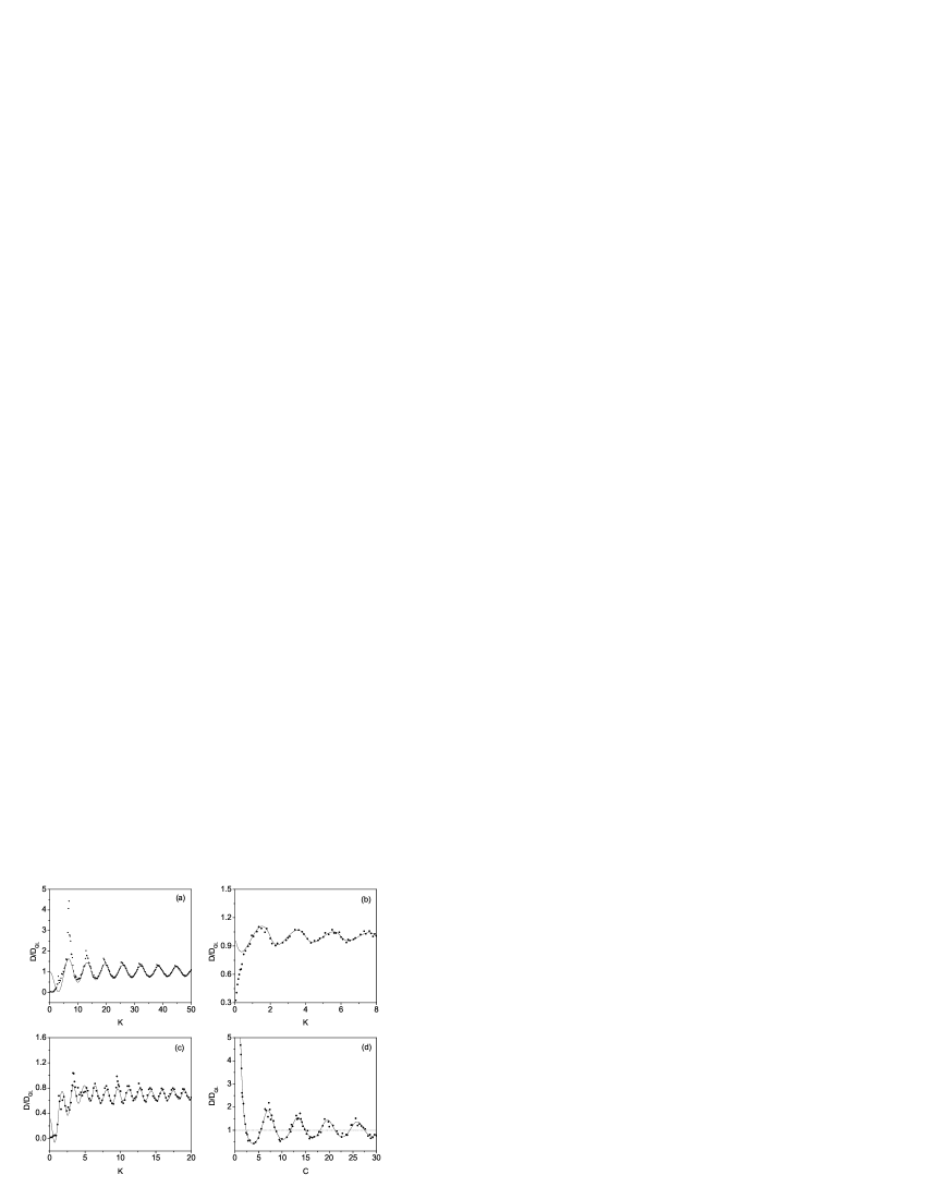
Figure 1: Theoretical diffusion coefficient rate $D/D_{ql}$ (solid lines) compared with numerical simulations calculated for $n=100$. In the cases (a), (b), and (c) we truncate the diffusion formulas (13) and (14) at $j=2$. A better agreement for small values of $K$ requires the calculation of further memory functions. (a) Standard map. The accelerator modes give rise to spikes in the figure. (b) Sawtooth map and (c) Harper map for $c=5.5$ (with presence of accelerator modes). (d) Harper map as a function of $c$ for $K=10^{5}$. The angular evolution induces fast and slow modes of diffusion even in the high stochasticity regime. This strong angular memory effect decay as $2J_{0}(c)/[1-J_{0}(c)]$.

References

- (1) B.V. Chirikov, Phys. Reports 52, 265 (1979).
- (2) A.B. Rechester and R.B. White, Phys. Rev. Lett. 44, 1586 (1980); A.B. Rechester, M.N. Rosenbluth and R.B. White, Phys. Rev. A 23, 2664 (1981).
- (3) H.D.I. Abarbanel, Physica 4D, 89 (1981).
- (4) J.R. Cary, J.D. Meiss, and A. Bhattacharjee, Phys. Rev. A 23, 2744 (1981); J.R. Cary and J.D. Meiss, Phys. Rev. A 24, 2664 (1981); J.D. Meiss, J.R. Cary, C. Grebogi, J.D. Crawford, A.N. Kaufman, and H.D.I. Abarbanel, Physica D 6, 375 (1983).
- (5) R.S. Mackay, J.D. Meiss, and I.C. Percival, Phys. Rev. Lett. 52, 697 (1984).
- (6) I. Dana, N.W. Murray, and I.C. Percival, Phys. Rev. Lett. 62, 233 (1990); I. Dana , Phys. Rev. Lett. 64, 2339 (1990); Q. Chen, I. Dana, J.D. Meiss, N.W. Murray, and I.C. Percival, Physica D 46, 217 (1990).
- (7) T. Hatori, T. Kamimura and Y.H. Hichikawa, Physica D 14, 193 (1985). The authors conclude that, for in (3), the diffusion coefficient relaxes to the quasilinear value for any nonlinear . They do not take into consideration the possibility of periodicity in .
- (8) P. Gaspard, Chaos, Scattering and Statistical Mechanics (Cambridge University Press, Cambridge, England, 1998).
- (9) J.R. Dorfman, An Introduction to Chaos in Nonequilibrium Statistical Mechanics (Cambridge University Press, Cambridge, England, 1999).
- (10) M. Pollicott, Invent. Math. 81, 413 (1985); Invent. Math. 85, 147 (1986).
- (11) D. Ruelle, Phys. Rev. Lett. 56, 405 (1986); J. Stat. Phys. 44, 281 (1986).
- (12) H.H. Hasegawa and W.C. Saphir, Phys. Rev. A 46, 7401 (1992).
- (13) P. Cvitanovi, J.-P. Eckmann and P. Gaspard, Chaos, Solitons and Fractals 6 113 (1995).
- (14) S. Tasaki and P. Gaspard, J. Stat. Phys. 81 935 (1995).
- (15) M. Khodas and S. Fishman, Phys. Rev. Lett. 84, 2837 (2000); M. Khodas, S. Fishman and O. Agam, Phys. Rev. E 62, 4769 (2000).
- (16) J. Weber, F. Haake, P. Seba, Phys. Rev. Lett. 85, 3620 (2000); J. Phys. A: Math. Gen. 34, 7195 (2001).
- (17) G. Blum, O. Agam, Phys. Rev. E 62, 1977 (2000).
- (18) K. Pance, W. Lu, S. Sridhar, Phys. Rev. Lett. 85, 2737 (2000).
- (19) A.J. Lichtenberg and M.A. Lieberman, Regular and Chaotic Dynamics (Springer, New York, 1992).
- (20) J.L. Zhou, Y.S. Sun, J.Q. Zheng, and M.J. Valtonen, Astron. Astrophys. 364, 887 (2000); B.V. Chirikov and V.V. Vecheslavov, Astron. Astroph. 221, 146 (1989); T.Y. Petrosky, Phys. Lett. A 117, 328 (1986).
- (21) A. Punjabi, A. Verma, and A. Boozer, Phys. Rev. Lett. 69, 3322 (1992); D. del-Castillo-Negrette and P.J. Morrison, Phys. Fluids A 5, 948 (1993); J.T. Mendonça, Phys. Fluids B 3, 87 (1991); H. Wobig and R.H. Fowler, Plasma Phys. Control. Fusion 30, 721 (1988).
- (22) A. Veltri and V. Carbone, Phys. Rev. Lett. 92, 143901 (2004); A.P.S. de Moura and P.S. Letelier, Phys. Rev. E 62, 4784 (2000); E. Fermi, Phys. Rev. 75, 1169 (1949); J.S. Berg, R.L. Warnock, R.D. Ruth and E. Forest, Phys. Rev. E 49, 722 (1994).
- (23) H.H. Hasegawa and W.C. Saphir, Aspects of Nonlinear Dynamics: Solitons and Chaos (193), edited by I. Antoniou and F. Lambert, (Springer, Berlin, 1991); R. Balescu, Statistical Dynamics, Matter out of Equilibrium (Imperial College Press, London, 1997).
- (24) It is a necessary condition for the validity of the Kol’mogorov-Arnol’d-Moser theorem on (3). In particular, this condition guarantees that rotational invariant circles with sufficiently irrational frequency persist under small -perturbations. For more details, see J. Moser, Stable and Random Motions in Dynamical Systems (Princeton University, Princeton, 1973).
- (25) V.I. Arnold and A. Avez, Ergodic Problems of Classical Mechanics (Benjamin, New York, 1968).
- (26) G.M. Zaslavsky, Phys. Rep. 371, 461 (2002).
- (27) R. Venegeroles (to be published).
- (28) J.A. McLennan, Introduction to Non-Equilibrium Statistical Mechanics (Prentice Hall, Engewood cliffs, New Jersey, 1989).
- (29) R. Venegeroles, Non-Gaussian Features of the Hamiltonian Transport (to be published).