Dynamics on unbounded domains;
co-solutions and inheritance of stability

Abstract

We consider the dynamics of semiflows of patterns on unbounded domains that are equivariant under a noncompact group action. We exploit the unbounded nature of the domain in a setting where there is a strong ‘global’ norm and a weak ‘local’ norm. Relative equilibria whose group orbits are closed manifolds for a compact group action need not be closed in a noncompact setting; the closure of a group orbit of a solution can contain ‘co-solutions’.

The main result of the paper is to show that co-solutions inherit stability in the sense that co-solutions of a Lyapunov stable pattern are also stable (but in a weaker sense). This means that the existence of a single group orbit of stable relative equilibria may force the existence of quite distinct group orbits of relative equilibria, and these are also stable. This is in contrast to the case for finite dimensional dynamical systems where group orbits of relative equilibria are typically isolated.

1 Introduction

There has been much effort devoted to trying to understand the dynamics of spatially extended systems; that is, dynamical systems that have not just unbounded time but also unbounded space dependence. Most of this work has progressed by restricting to parabolic partial differential equations such as the Ginzburg-Landau and Swift-Hohenberg equations (see for example [9, 5]) used to model ‘generic’ instabilities with nontrivial spatial dependence. This has been successful in characterising solutions of specific types in specific systems of equations; for example wave-like solutions, fronts between them [3], spirals and defects. Related to this approach there have been attempts to find a ‘qualitative theory’ of partial differential equations (see for example [4]) where careful reductions to ODE models can explain many universal features of patterns in unbounded systems, for example the stability of fronts and defects [11].

There remain fundamental problems in trying to characterise what sort of attractors ‘generically’ appear in initial value problems for partial differential equations with unbounded domains. Related to this is the usual problem of deciding which space of functions and which topology or norm is appropriate. As is well recognised, a change of choice of norm can lead to qualitatively very different behaviour [10, 9]. For example, consider a solution $u(x,t)$ to the heat equation $u_{t}=u_{xx}$ with initial condition $u_{0}(x)\geq 0$ satisfying $\int|u_{0}(x)|\,dx<\infty$. Then $u(x,t)$ decays to zero in sufficiently ‘weak’ norms; for example a weighted $L^{1}$ norm $\|u\|={\textstyle\int}\rho(x)|u(x,t)|\,dx$ with weight $\rho>0$ such that $\rho(x)\rightarrow 0$ as $|x|\rightarrow\infty$. By contrast in a more ‘global’ norm such as the $L^{1}$ norm, the solution remains bounded away from zero.

Rather than being discouraged by what might be seen as the arbitrary nature of the choice of topology, in this paper we wish to use it to our advantage. In an attempt to move away from specific systems of equations we consider a general setting where the dynamics is given by a semiflow on a space of patterns. A key assumption is that there are two important topologies; a weak one which characterises local changes and a strong one which characterises global changes. We assume that the semiflow is continuous for both of the topologies and note that this is typical in many systems.

If there is a stable propagating front between states $A$ and $B$ it seems reasonable to ask whether $A$ and $B$ inherit the stability of the front. We describe a setting in which one can make such deductions and extend them to understand the stability in general for ‘far field’ stable patterns.

In many models for dynamics on unbounded domains there are translational or Euclidean group symmetries in the model. We make an assumption of this form to allow us to discuss a range of different solutions. We assume that the semiflow commutes with the action of a noncompact group $\Gamma$, meaning that we can characterise the unboundedness by group symmetries.

Section 2 gives the details of the setting and some motivating examples. Section 3 shows that under quite general assumptions on the semiflow, solutions often force the existence of a variety of new solutions that we call co-solutions. These co-solutions are patterns that are in the closure of the group orbit in the weak topology. In Proposition 3.3 we give conditions such that if the original solution is a relative equilibrium then the co-solution is also a relative equilibrium. The main result in Section 4 shows that the stability of a solution implies stability of its co-solutions. Section 5 discusses the results and suggests some further questions that may be usefully addressed using this approach.

2 Semiflows with noncompact domain symmetries

We consider the behaviour of patterns that evolve on an infinite domain for a semiflow equivariant under a group $\Gamma$ acting on this domain. By a space of patterns we mean a vector space $\mathcal{B}$ of functions $u:D\to{\mathbb{R}}^{s}$ where for example $D={\mathbb{R}}^{n}$. We suppose that $\Gamma$ is a (noncompact) Lie group acting on $\mathcal{B}$ and $L\Gamma$ is the Lie algebra of $\Gamma$. Our main applications have $D={\mathbb{R}}^{n}$ and $\Gamma={\bf E}(n)$ or ${\bf SE}(n)$.

2.1 The strong and weak topologies

We consider semiflows on $\mathcal{B}$ subject to two topologies that express closeness in a weak (local) or in a strong (global) senses. More precisely, we assume:

• • The strong norm $\|.\|_{s}$ is $\Gamma$-invariant, i.e. $\|\gamma u\|_{s}=\|u\|_{s}$ for all $u\in\mathcal{B}$ and $\gamma\in\Gamma$.

  • For each fixed $\gamma\in\Gamma$, the linear map $u\mapsto\gamma u$ is bounded in the weak norm. (So $\|\gamma u\|_{w}\leq K\|u\|_{w}$ for all $u\in\mathcal{B}$, where $K=\|\gamma\|_{w}<\infty$ is the operator norm of $\gamma$.)

  • The map $\gamma\to\|\gamma\|_{w}$ is continuous.

• There is a family of functions $\Lambda=\{\lambda\}$ of functions $\lambda:D\rightarrow(0,\infty)$ such that

  • $\|u\|_{w}\leq\|\lambda u\|_{s}\leq\|u\|_{s}$, and

  • For all $M>0$ and $\epsilon>0$, there exists $\lambda\in\Lambda$ such that

    $$\|u\|_{s}\leq M\enspace\text{implies that}\enspace\|(1-\lambda)u\|_{w}<\epsilon.$$

• For all $u\in\mathcal{B}$, $v\in\operatorname{clos}_{w}(\Gamma u)$, $\lambda\in\Lambda$ and $\epsilon>0$, there exists $\gamma\in\Gamma$ such that

  $$\|\lambda(\gamma u-v)\|_{s}<\epsilon.$$

We give an example of a setting of weighted norms where these hypotheses can be verified in Section 2.3 below. In our example, $\mathcal{B}$ is a Banach space under the strong norm but not the weak norm. This is the typical situation for the applications we have in mind, but completeness is not used in this paper.

2.2 Dynamics on $\mathcal{B}$

Suppose that we have an evolution given by a semiflow $\Phi_{t}:\mathcal{B}\rightarrow\mathcal{B}$ such that

$$\Phi_{t}\circ\Phi_{s}=\Phi_{s+t},~{}~{}\Phi_{0}={\rm Id}.$$

We suppose that $\Phi_{t}$ is continuous in both the weak norm $\|.\|_{w}$ and the strong norm $\|.\|_{s}$ on the function space $\mathcal{B}$. We suppose also that $\Phi_{t}$ is $\Gamma$-equivariant.

We say $u\in\mathcal{B}$ has symmetry or isotropy $\Sigma_{u}=\{\gamma\in\Gamma~{}:~{}\gamma u=u\}$ (see for example [7]). A subgroup $\Sigma$ of $\Gamma$ is cocompact if the coset space $\Gamma/\Sigma$ is compact.

We say $u_{0}\in\mathcal{B}$ is a relative equilibrium if $\Phi_{t}(u_{0})=u(t)=e^{\eta t}u_{0}$ for some $\eta\in L\Gamma$ which is called the drift of $u_{0}$. Note that for any $\gamma\in\Gamma$, $\gamma u_{0}$ is also a relative equilibrium with drift $\eta_{\gamma}$, where $\eta_{\gamma}$ is given by the adjoint action of $\gamma$ on $\eta$ (i.e. $e^{\eta_{\gamma}t}=\gamma e^{\eta t}\gamma^{-1}$ for all $t>0$.)

Remark 2.1

Associated to the relative equilibrium $u(t)=e^{\eta t}u_{0}$ is the closed Lie subgroup

$$K(\eta)=\overline{\{\exp\eta t~{}:~{}t\in{\mathbb{R}}\}}.$$

Recall that for $\Gamma$ compact and any $\eta$ the group $K(\eta)$ is a torus and for generic $\eta$ this torus is maximal [6, 8]. For $\Gamma$ non-compact, $K(\eta)$ is either isomorphic to ${\mathbb{R}}$ or to a torus; generically $K(\eta)$ is either a maximal torus or ${\mathbb{R}}$, see [2]. For ${\bf E}(n)$, generically $K(\eta)$ is a torus for $n$ even, and generically $K(\eta)\cong{\mathbb{R}}$ for $n$ odd.

2.3 An example in ${\mathbb{R}}^{n}$ satisfying (H1)–(H3)

Let $\mathcal{B}$ be a set of functions $u:{\mathbb{R}}^{n}\to{\mathbb{R}}^{s}$. We assume that $\Gamma$ is a closed subgroup of ${\bf E}(n)$ acting as Euclidean isometries in the domain variables ${\mathbb{R}}^{n}$, possibly coupled with a norm-preserving action in the range ${\mathbb{R}}^{s}$. More precisely, let $\gamma=(A,a)\in{\bf E}(n)={\bf O}(n)\ltimes{\mathbb{R}}^{n}$ act on $x\in{\mathbb{R}}^{n}$ by $\gamma x=Ax+a$, and let $\chi:\Gamma\to O(s)$ be an orthogonal action of $\Gamma$ on ${\mathbb{R}}^{s}$. Then we assume that the action of $\gamma$ on functions $u\subset\mathcal{B}$ is given by

$$(\gamma u)(x)=(\chi_{\gamma}u)(\gamma^{-1}x).$$

Define the strong norm $\|u\|_{s}=\sup_{x}|u(x)|$ and the weak norm $\|u\|_{w}=\|\rho u\|_{s}$ where $\rho(x)=(1-|x|^{2})^{-1}$ and $|x|^{2}=x_{1}^{2}+\dots+x_{n}^{2}$. We also define the family of weights $\lambda_{\alpha}(x)=\rho(\alpha x)$, $0<\alpha\leq 1$.

Lemma 2.2

In this setting, hypotheses (H1)–(H3) are satisfied with $\Lambda=\{\lambda_{\alpha}:0<\alpha\leq 1\}$.

Proof.

Let $\gamma\in\Gamma$, $u\in\mathcal{B}$. It follows from orthogonality of the action $\chi$ on ${\mathbb{R}}^{s}$ that $|(\gamma u)(x)|=|u(\gamma^{-1}x)|$. In particular, $\|\gamma u\|_{s}=\|u\|_{s}$ proving (H1)(a).

For any $a\in{\mathbb{R}}^{n}$, $\lim_{|x|\to\infty}\rho(x+a)/\rho(x)=1$ so we can define $C(a)=\sup_{x}\rho(x+a)/\rho(x)<\infty$. Writing $\gamma x=Ax+a=A(x+A^{-1}a)$, we claim that $\|\gamma\|_{w}=C(A^{-1}a)$. It suffices to show that $\|\gamma\|_{w}=1$ for $\gamma x=Ax$ and $\|\gamma\|_{w}=C(a)$ for $\gamma x=x+a$.

Note that $\|\gamma u\|_{w}=\sup_{x}\rho(x)|u(\gamma^{-1}x)|=\sup_{x}\rho(\gamma x)|u(x)|$. If $\gamma x=Ax$, then $\rho(\gamma x)=\rho(x)$ and $\|\gamma\|_{w}=1$. If $\gamma x=x+a$ is a translation, then it follows from the definition of $C(a)$ that $\|\gamma u\|_{w}=C(a)$. This completes the proof of (H1)(b).

It is clear that $C(a)$ depends continuously on $a$ so that $\|\gamma\|_{w}$ depends continuously on $\gamma$, proving (H1)(c).

Let $\alpha>0$ and note that for any $x$

$$|\rho(x)u(x)|\leq|\lambda_{\alpha}u(x)|\leq|u(x)|$$

proving (H2)(a). To verify (H2)(b), suppose that $\|u\|_{s}<M$ so that

$$\|(1-\lambda_{\alpha})u\|_{w}=\sup_{x}|\rho(x)(1-\lambda_{\alpha}(x))u(x)|\leq P_{\alpha}M$$

where

$$P_{\alpha}=\sup_{r}\frac{1}{1+r^{2}}\,\frac{\alpha^{2}r^{2}}{1+\alpha^{2}r^{2}}\leq\alpha^{2}.$$

Hence $P_{\alpha}\rightarrow 0$ as $\alpha\rightarrow 0$, and so we can choose $\lambda=\lambda_{\alpha}$ with $\alpha$ sufficiently small.

For (H3), let $M=\|u\|_{s}+\|v\|_{s}$. Since $v\in\operatorname{clos}_{w}(\Gamma u)$, there is a sequence $\gamma_{n}$ such that $\gamma_{n}u-v\to_{w}0$. In particular, $\gamma_{n}u-v\to 0$ pointwise. Moreover, $\sup_{x}|\gamma_{n}u(x)-v(x)|\leq M$ and so it is easy to verify that $\lambda(\gamma_{n}u-v)\to 0$ uniformly for each fixed $\lambda\in\Lambda$ as required. ∎

It is routine to extend this result to the case of a $C^{k}$ norm, $k\geq 1$. As a trivial example of a semiflow that evolves continuously on $\mathcal{B}$, take any semiflow that evolves continuously according to its local value, i.e. such that

$$(\Phi_{t}(u))(x)=F_{t}(u(x))$$

where $F_{t}$ is a continuous semiflow on ${\mathbb{R}}^{s}$. Less trivial examples are given by solutions of reaction-diffusion systems.

3 Co-solutions and relative equilibria

Suppose that $\Phi_{t}$ is a semiflow on $\mathcal{B}$ that is continuous in strong and weak norms satisfying the hypotheses in Section 2.

For continuous action of compact groups, relative equilibria are compact and hence closed. As noted in [2], this is not true for noncompact groups unless one makes further assumptions. Generally speaking, in the situations of interest in this paper, the relative equilibria are closed in the strong topology but not in the weak topology.

Definition 3.1

Let $u_{0},v_{0}\in\mathcal{B}$. We say that $v_{0}$ is a co-solution of $u_{0}$ if $v_{0}\in\operatorname{clos}_{w}(\Gamma u_{0})$.

If $u_{0},v_{0}\in\mathcal{B}$ and $u(t)=\Phi_{t}(u_{0})$, $v(t)=\Phi_{t}(v_{0})$ are the corresponding solutions, then we say that $v(t)$ is a co-solution of $u(t)$ if $v_{0}$ is a co-solution of $u_{0}$. It follows from weak-continuity of the flow that the property $v(t)\in\operatorname{clos}_{w}(\Gamma u(t))$ holds for one value of $t$ if and only if it holds for all $t$. Hence the set of co-solutions of any given solution is also an invariant set.

Remark 3.2

(a) Note that $v_{0}$ being a co-solution for $u_{0}$ means that one can find arbitrarily large patches of $u_{0}$ that resemble $v_{0}$ arbitrarily closely, up to transformation by elements of $\Gamma$.
(b) Our definition of co-solution is in terms of the weak topology. We can also define a strong notion of co-solution. However in many situations of interest, the notion is vacuous. Indeed, suppose that $u_{0}$ is a relative equilibrium with isotropy $\Sigma$. Following [2, Definition 5.2], we say that a sequence $\{\gamma_{n}\}\subset\Gamma/\Sigma$ is an approximate symmetry of $u_{0}$ if $\gamma_{n}$ has no convergent subsequences and $\|\gamma_{n}u_{0}-u_{0}\|_{s}\to 0$. If no such approximate symmetries exist, then in the strong topology $\Gamma u_{0}$ is a closed submanifold diffeomorphic to $\Gamma/\Sigma$ (see [2, Proposition 5.3]).
(c) Arguing as in (b), we note that relative equilibria with cocompact isotropy subgroup are compact and hence closed in both the strong and weak topologies. In particular, such relative equilibria cannot have nontrivial co-solutions.

It is clear the co-solutions of equilibria are themselves equilibria. In certain cases, co-solutions of relative equilibria are also relative equilibria.

Proposition 3.3

Suppose $u_{0}$ is a relative equilibrium with drift $\xi$. If there is a sequence $\gamma_{n}\in\Gamma$, an $\eta\in L\Gamma$ and a $v_{0}\in\mathcal{B}$ such that $\|\gamma_{n}u_{0}-v_{0}\|_{w}\rightarrow 0$ and

$$\|(e^{\xi_{n}t}-e^{\eta t})\gamma_{n}u_{0}\|_{w}\rightarrow 0$$

as $n\rightarrow\infty$ (where $\xi_{n}=\xi_{\gamma_{n}}$ is the drift of $\gamma_{n}u_{0}$) for all $t>0$, then $v_{0}$ is a relative equilibrium with drift $\eta$.

Proof.

We set $u_{n}=\gamma_{n}u_{0}$ and calculate

$$\|e^{\eta t}v_{0}-\Phi_{t}(v_{0})\|_{w} = \|e^{\eta t}v_{0}-e^{\eta t}u_{n}+e^{\eta t}u_{n}-e^{\xi_{n}t}u_{n}+e^{\xi_{n}t}u_{n}-\Phi_{t}(v_{0})\|_{w}$$

$$\leq \|e^{\eta t}v_{0}-e^{\eta t}u_{n}\|_{w}+\|e^{\eta t}u_{n}-e^{\xi_{n}t}u_{n}\|_{w}+\|\Phi_{t}(u_{n})-\Phi_{t}(v_{0})\|_{w}.$$

In the limit $n\rightarrow\infty$ for fixed $t$, by continuity of the group action the first term goes to zero, by the hypothesis the second term goes to zero and by continuity of the flow the third term goes to zero. Hence

$$\Phi_{t}(v_{0})=e^{\eta t}v_{0}$$

meaning that $v_{0}$ is a relative equilibrium with drift $\eta$. ∎

Remark 3.4

(a) A special case where Proposition 3.3 applies is when $v_{0}\in\operatorname{clos}_{w}(\Gamma u_{0})$ and $v$ has a drift that is in the centre of $\Gamma$. In such a case $\xi_{n}=\xi$ and we can choose $\eta=\xi$ to satisfy the hypotheses.
(b) Another special case satisfying these hypotheses is where $v$ has full symmetry, in which case $\eta=0$.

3.1 Examples of co-solutions

To motivate the results we give a few examples of patterns that have a nontrivial set of co-solutions, building on ideas in [1]. Figure 1 shows two examples. Figure 1(a) shows a front between a spatially periodic pattern for $x>0$ and a uniform state for $x<0$. If this pattern is a relative equilibrium for a flow that fits our setting then there are two families of co-solutions; the uniform pattern for $x\to-\infty$ and the periodic pattern for $x\to+\infty$. Figure 1(b) shows a defect solution that implies the existence of stripe solutions as well. Note that in both cases all co-solutions have cocompact symmetry, so the co-solutions have no further co-solutions.

 

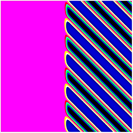
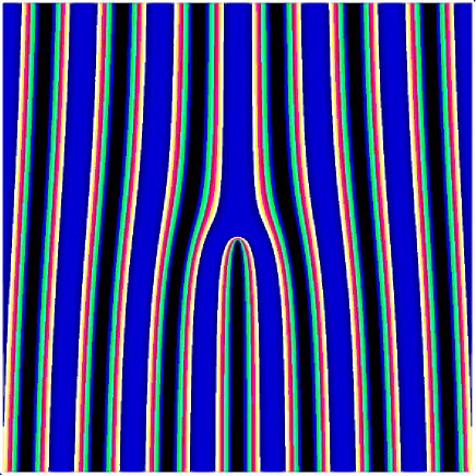
(a)                                                                     (b)

Figure 1: (a) A relative equilibrium for a Euclidean-equivariant system with two co-solutions that are relative equilibria; a uniform state (by taking translations to the right) and a family of spatially periodic states (by taking translations to the left). (b) A relative equilibrium that is a defect of this form has stripe co-solutions that are relative equilibira on taking translations in any direction. In both cases the co-solutions have additional symmetries.

Another example is illustrated in Figure 2; this shows one component of reaction diffusion system with a spiral relative equilibrium that rotate anticlockwise. By taking limits of large translations in any direction we obtain weak co-solutions that are propagating spatially periodic stripe patterns.

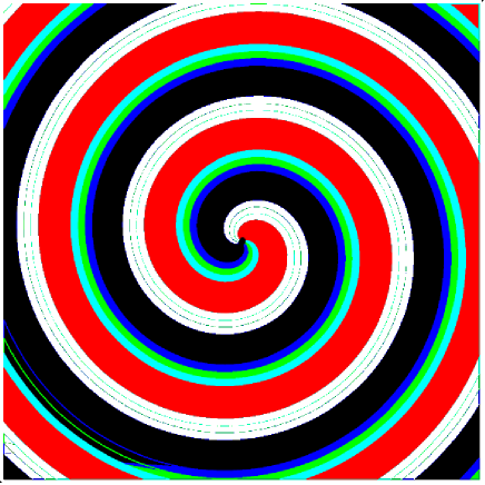
Figure 2: A spiral relative equilibrium for a Euclidean-equivariant system with co-solutions given by rolls that drift if the spiral rotates; these are be found by considering translates of the spiral in any direction.

3.2 Symmetries of co-solutions

In spite of the fact that co-solutions are generated by symmetries of the system there is not a simple relationship between the symmetries of a relative equilibrium $v$ and the symmetries of a co-solution. Figures 1 and 2 show cases where the co-solutions have more symmetry than the original pattern. By contrast Figure 3 has a reflection symmetry in the vertical axis that is missing on the cosolutions obtained by translating to the left or right. Hence symmetry may be gained or lost in passing from a relative equilibrium to a co-solution.

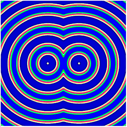
Figure 3: Consider an equilibrium for a Euclidean-equivariant system that has two target patterns anchored near each other. Observe that this has co-solutions that are spatially periodic stripe patterns; moreover the vertical axis reflection symmetry of the original pattern is missing in taking the stripe pattern cosolutions.

4 Inheritance of stability

Let $u_{0}\in\mathcal{B}$. We say that $u_{0}$ is (Lyapunov) sw-stable if for all $\epsilon>0$ there exists $\delta>0$ such that

$$\|u-u_{0}\|_{s}<\delta\enspace\text{implies that}\enspace\|\Phi_{t}(u)-\Phi_{t}(u_{0})\|_{w}<\epsilon\enspace\text{for all $t>0$}.$$ (1)

Similarly, we say $u_{0}$ is ss-stable if (1) holds with $\|.\|_{w}$ replaced by $\|.\|_{s}$. This corresponds to the usual notion of stability. Observe that ss-stability clearly implies sw-stability.

In a similar way one could define ww-stability but this is probably too weak to be of use and so we do not discuss it further here.

Proposition 4.1

If $u_{0}\in\mathcal{B}$ is sw-stable (resp. ss-stable) then so is $\gamma u_{0}$ for all $\gamma\in\Gamma$.

Proof.

Suppose that $u_{0}$ is sw-stable and $\gamma\in\Gamma$. By (H1)(b), $K=\|\gamma\|_{w}<\infty$. For any $\epsilon>0$, there exists $\delta>0$ such that $\|u-u_{0}\|_{s}<\delta$ implies that $\|\Phi_{t}(u)-\Phi_{t}(u_{0})\|_{w}<\epsilon/K$ for all $t>0$.

We show that $v_{0}=\gamma u_{0}$ is sw-stable. Suppose that $\|v-v_{0}\|_{s}<\delta$. By (H1)(a), $\|\gamma^{-1}v-u_{0}\|_{s}<\delta$. Hence $\|\Phi_{t}(\gamma^{-1}v)-\Phi_{t}(u_{0})\|_{w}<\epsilon/K$. By (H1)(b) and equivariance of the flow,

$$\|\Phi_{t}(v)-\Phi_{t}(v_{0})\|_{w}\leq K\|\gamma^{-1}(\Phi_{t}(v)-\Phi_{t}(v_{0}))\|_{w}=K\|\Phi_{t}(\gamma^{-1}v)-\Phi_{t}(u_{0})\|<K\epsilon/K=\epsilon,$$

proving that $v_{0}$ is sw-stable.

The proof that ss-stability of $u_{0}$ is inherited by $v_{0}$ is simpler (with $K=1$) by (H1)(a). ∎

Theorem 4.2

Suppose that $u_{0},v_{0}\in\mathcal{B}$ and $v_{0}\in\operatorname{clos}_{w}(\Gamma u_{0})$. If $u_{0}$ is ss-stable then $v_{0}$ is sw-stable.

Proof.

We prove the statement by contradiction, assuming that $v_{0}$ is sw-unstable and arguing that $u_{0}$ must be ss-unstable.

Since $v_{0}$ is sw-unstable, there is an $\epsilon>0$ such that for all $\delta>0$ we can find a $T>0$ and $v_{1}$ (both depending on $\delta$) such that

$$\|v_{1}-v_{0}\|_{s}<\delta,$$ (2)

but

$$\|\Phi_{T}(v_{1})-\Phi_{T}(v_{0})\|_{w}\geq\epsilon.$$ (3)

By weak continuity of $\Phi_{t}$, there exists $\eta\in(0,\delta)$ such that

$$\|\Phi_{T}(z)-\Phi_{T}(v_{0})\|_{w} <\frac{\epsilon}{3}\quad\text{for all $z\in\mathcal{B}$ with $\|z-v_{0}\|_{w}<\eta$},$$ (4)

$$\|\Phi_{T}(z)-\Phi_{T}(v_{1})\|_{w} <\frac{\epsilon}{3}\quad\text{for all $z\in\mathcal{B}$ with $\|z-v_{1}\|_{w}<\eta$}.$$ (5)

Set $M=\|u_{0}\|_{s}+\|v_{1}\|_{s}$. Then $\|\gamma u_{0}-v_{1}\|_{s}\leq M$ for all $\gamma\in\Gamma$ by (H1)(a), and hence by (H2)(b) there exists $\lambda_{0}\in\Lambda$ such that

$$\|(1-\lambda_{0})(\gamma u_{0}-v_{1})\|_{w}<\eta\quad\text{for all $\gamma\in\Gamma$}.$$ (6)

Since $v_{0}\in\operatorname{clos}_{w}(u_{0})$, it follows from (H3) that there exists $\gamma_{0}\in\Gamma$ such that

$$\|\lambda_{0}(\gamma_{0}u_{0}-v_{0})\|_{s}<\eta<\delta.$$ (7)

By hypothesis (H2)(a) and estimate (7),

$$\|\gamma_{0}u_{0}-v_{0}\|_{w}\leq\|\lambda_{0}(\gamma_{0}u_{0}-v_{0})\|_{s}<\eta,$$

so it follows from (4) that

$$\|\Phi_{T}(\gamma_{0}u_{0})-\Phi_{T}(v_{0})\|_{w}<\frac{\epsilon}{3}.$$ (8)

Now define

$$u_{1}=(1-\lambda_{0})\gamma_{0}u_{0}+\lambda_{0}v_{1}.$$

Then $u_{1}-\gamma_{0}u_{0}=\lambda_{0}(v_{1}-\gamma_{0}u_{0})$ and we compute that

$$\|\gamma_{0}^{-1}u_{1}-u_{0}\|_{s} =\|u_{1}-\gamma_{0}u_{0}\|_{s}=\|\lambda_{0}(v_{1}-\gamma_{0}u_{0})\|_{s}\ \leq\|\lambda_{0}(v_{1}-v_{0})\|_{s}+\|\lambda_{0}(\gamma_{0}u_{0}-v_{0})\|_{s}$$

$$\leq\|v_{1}-v_{0}\|_{s}+\|\lambda_{0}(\gamma_{0}u_{0}-v_{0})\|_{s}<\delta+\delta=2\delta,$$

where we have used hypotheses (H1)(a) and (H2)(a), and estimates (2) and (7).

Moreover, $u_{1}-v_{1}=(1-\lambda_{0})(\gamma_{0}u_{0}-v_{1})$ so $\|u_{1}-v_{1}\|_{w}<\eta$ by (6). It follows from (5) that

$$\|\Phi_{T}(u_{1})-\Phi_{T}(v_{1})\|_{w}<\frac{\epsilon}{3}.$$ (9)

Writing

$$\Phi_{T}(u_{1})-\Phi_{T}(\gamma_{0}u_{0})=[\Phi_{T}(u_{1})-\Phi_{T}(v_{1})]+[\Phi_{T}(v_{1})-\Phi_{T}(v_{0})]+[\Phi_{T}(v_{0})-\Phi_{T}(\gamma_{0}u_{0})]$$

we have

$$\|\Phi_{T}(\gamma_{0}^{-1}u_{1})-\Phi_{T}(u_{0})\|_{s}=\|\Phi_{T}(u_{1})-\Phi_{T}(\gamma_{0}u_{0})\|_{s}$$

$$\qquad\geq\|\Phi_{T}(v_{1})-\Phi_{T}(v_{0})\|_{w}-\|\Phi_{T}(u_{1})-\Phi_{T}(v_{1})\|_{w}-\|\Phi_{T}(\gamma_{0}u_{0})-\Phi_{T}(v_{0})\|_{w}$$

$$\qquad\geq\epsilon-\frac{\epsilon}{3}-\frac{\epsilon}{3}=\frac{\epsilon}{3},$$

where we have used hypothesis (H1)(a), $\Gamma$-equivariance of $\Phi_{T}$, and estimates (5), (8) and (9).

Summarizing, we have shown that there is an $\epsilon>0$ such that for all $\delta>0$ there is a $T>0$ and a $w=\gamma_{0}^{-1}u_{1}$ such that

$$\|w-u_{0}\|_{s}<2\delta\quad\text{and}\quad\|\Phi_{T}(w)-\Phi_{T}(u_{0})\|_{s}\geq\frac{\epsilon}{3}$$

giving ss-instability of $u_{0}$ and the proof is complete. ∎

In certain situations we obtain a more powerful result, namely in the presence of an additional hypothesis:

• For any $\epsilon>0$, there exists $\delta>0$ such that for any $u\in\mathcal{B}$

  $${\textstyle\sup_{\gamma\in\Gamma}}\|\gamma u\|_{w}<\delta\enspace\text{implies that}\enspace\|u\|_{s}<\epsilon.$$

Note that hypothesis (H4) clearly holds for the setup in Section 2.3 where we have $\|u\|_{s}=\sup_{\gamma\in\Gamma}\|\gamma u\|_{w}$.

Lemma 4.3

Suppose that (H1-H4) hold and that $u_{0}\in\mathcal{B}$ has cocompact isotropy $\Sigma$. Then $u_{0}$ is ss-stable if and only if $u_{0}$ is sw-stable.

Proof.

We prove the nontrivial direction, namely that sw-stability implies ss-stability. Let $\epsilon>0$ and choose $\delta>0$ as in (H4). By Proposition 4.1, $\gamma u_{0}$ is sw-stable for all $\gamma\in\Gamma$. Hence, for each $\gamma$, there exists $\eta=\eta(\gamma)>0$ such that $\|u-\gamma u_{0}\|_{s}<\eta$ implies that $\|\Phi_{t}(u)-\Phi_{t}(\gamma u_{0})\|_{w}<\delta$ for all $t>0$. By the proof of Proposition 4.1, we can take $\eta(\gamma)=\eta(1_{\Gamma})/\|\gamma\|_{w}$ where $1_{\Gamma}$ is the identity element in $\Gamma$. By (H1)(c), $\eta(\gamma)$ depends continuously on $\gamma$. Clearly $\eta(\gamma)$ can be chosen to be constant on $\Sigma$-cosets. Since $\Gamma/\Sigma$ is compact, it follows that $\eta>0$ can be chosen independent of $\gamma$.

Suppose that $\|v-u_{0}\|_{s}<\eta$ and let $\gamma\in\Gamma$. By hypothesis (H1)(a), $\|\gamma v-\gamma u_{0}\|_{s}<\eta$, so by the above argument with $u=\gamma v$ we have $\|\Phi_{t}(\gamma v)-\Phi_{t}(\gamma u_{0})\|_{w}<\delta$ for all $t>0$. By equivariance, $\|\gamma(\Phi_{t}(v)-\Phi_{t}(u_{0}))\|_{w}<\delta$ for all $t>0$ and all $\gamma\in\Gamma$. By (H4), we deduce that $\|\Phi_{t}(v)-\Phi_{t}(u_{0})\|_{s}<\epsilon$ for all $t>0$ and so $u_{0}$ is ss-stable. ∎

Combining Theorem 4.2 and Lemma 4.3 we have:

Theorem 4.4

Suppose that $u_{0},v_{0}\in\mathcal{B}$ and $v_{0}\in\operatorname{clos}_{w}(\Gamma u_{0})$. Suppose further that $v_{0}$ has cocompact isotropy. If $u_{0}$ is ss-stable then $v_{0}$ is also ss-stable.

The means, for example, that the existence of an ss-stable relative equilibrium of the form in Figure 1(a) implies that both the uniform and the stripe co-solutions are ss-stable. Similarly if the spiral solution in Figure 2 is ss-stable then the ‘far field’ roll solutions are are ss-stable.

5 Discussion

We give a novel way of trying to understand the qualitative behaviour of dynamics on unbounded domains. There is clearly a great deal more that can be investigated by making use of a strong and a weak norm that satisfy assumptions such as (H1-H4) to a co-solution.

One direction that seems worth pursuing is the generalisation to transients. In particular initial conditions may converge to relative equilibria in a weak sense, and this gives further predictions for the existence of co-solutions (see for example the spiral wind-up discussed in [1]); we note that the results in Section 4 apply equally for solutions and co-solutions that are not relative equilibria.

In another direction, the results above are purely ‘topological’ in nature and do not attempt to understand the smooth dynamics. This setting may give a way to obtain results that relate smooth dynamical properties such as spectral stability to topological properties such as ss- and sw-stability and indeed to understand what qualitative ingredients a bifurcation theory for such systems should have.

Similarly it would be interesting to discuss asymptotic stability as well as Lyapunov stability in the setting; we observe that similar to the case for Lyapunov stability there will be several inequivalent notions of asymptotic stability depending on choice of norm.

Finally, we remark that there are situations where a flow that is continuous in the weak and strong topology becomes continuous in only the strong topology due to the appearance of mean flow effects [12]. At this point, certain of our hypotheses are violated, and it would be interesting to understand how this impacts on the relationship between local and global dynamics.

Acknowledgements

This research was supported in part by EPSRC research grant number GR/S31662 (PA) and by a Leverhulme Fellowship (IM).

References

• [1] P. Ashwin. Patchwork patterns: dynamics on unbounded domains. In: Proceedings of workshop on Symmetry and Bifurcation, Porto 2000, Editors: J Buescu, S Castro, A Dias and I Laboriau (Birkhauser 2003).
• [2] P. Ashwin and I. Melbourne. Noncompact drift for relative equilibria and relative periodic orbits. Nonlinearity 10, 595-616 (1997).
• [3] P. Collet and J.-P. Eckmann. Instabilities and Fronts in Extended Systems. Princeton University Press (1990).
• [4] P. Coullet, C. Riera and C. Tresser. Qualitative theory of stable stationary localised structures in one dimension. Prog. Theor. Phys 139, 46–49 (2000).
• [5] E. Feireisl, P. Laurençot and F. Simondon. Global attractors for degenerate parabolic equations on unbounded domains. J. Diff. Eqns. 129, 239–261 (1996).
• [6] M. J. Field. Equivariant dynamical systems. Trans. Amer. Math. Soc. 259, 185–205 (1980).
• [7] M. Golubitsky, I. N. Stewart and D. Schaeffer. Singularities and Groups in Bifurcation Theory, Vol. II, Appl. Math. Sci. 69, Springer, New York, 1988.
• [8] M. Krupa. Bifurcations of relative equilibria. SIAM J. Math. Anal. 21, 1453–1486 (1990).
• [9] A. Mielke. The Ginzburg-Landau equation in its role as a modulation equation. In B. Fiedler, editor, Handbook of Dynamical Systems II, pages 759-834. Elsevier Science B.V., (2002)
• [10] A. Mielke and G. Schneider. Attractors for modulation equations on unbounded domains – existence and comparison. Nonlinearity 8, 743–768 (1995).
• [11] B. Sandstede and A. Scheel. Essential instabilities of fronts: bifurcation, and bifurcation failure. Dynamical Systems 16, 1–28 (2001).
• [12] J. D. Scheel, M. R. Paul, M. C. Cross, and P. F. Fischer. Traveling waves in rotating Rayleigh-Bénard convection: Analysis of modes and mean flow. Phys. Rev. E 66 06621 (2003).