Loschmidt echo decay from local boundary perturbations

Abstract

We investigate the sensitivity of the time evolution of semiclassical wave packets in two-dimensional chaotic billiards with respect to local perturbations of their boundaries. For this purpose, we address, analytically and numerically, the time decay of the Loschmidt echo (LE). We find the LE to decay exponentially in time, with the rate equal to the classical escape rate from an open billiard obtained from the original one by removing the perturbation-affected region of its boundary. Finally, we propose a principal scheme for the experimental observation of the LE decay.

The study of the sensitivity of the quantum dynamics to perturbations of the system’s Hamiltonian is one of the important objectives of the field of Quantum Chaos. An essential concept here is the Loschmidt echo (LE), also known as fidelity, that was first introduced by Peres peres and has been widely discussed in the literature since then review . The LE, $M(t)$, is defined as an overlap of the quantum state $e^{-iHt/\hbar}|\phi_{0}\rangle$ obtained from an initial state $|\phi_{0}\rangle$ in the course of its evolution through a time $t$ under a Hamiltonian $H$, with the state $e^{-i\tilde{H}t/\hbar}|\phi_{0}\rangle$ that results from the same initial state by evolving the latter through the same time, but under a perturbed Hamiltonian $\tilde{H}$ different from $H$:

$$M(t)=\left|\langle\phi_{0}|e^{i\tilde{H}t/\hbar}e^{-iHt/\hbar}|\phi_{0}\rangle\right|^{2}.$$ (1)

It can be also interpreted as the overlap of the initial state $|\phi_{0}\rangle$ and the state obtained by first propagating $|\phi_{0}\rangle$ through the time $t$ under the Hamiltonian $H$, and then through the time $-t$ under $\tilde{H}$. The LE equals unity at $t=0$, and typically decays further in time.

Jalabert and Pastawski have analytically discovered jalab that in a quantum system, with a chaotic classical counterpart, Hamiltonian perturbations (sufficiently week not to affect the geometry of classical trajectories, but strong enough to significantly modify their actions) result in the exponential decay of the average LE $\overline{M(t)}$, where the averaging is performed over an ensemble of initial states or system Hamiltonians: $\overline{M(t)}\sim e^{-\lambda t}$. The decay rate $\lambda$ equals the average Lyapunov exponent of the classical system. This decay regime, known as the Lyapunov regime, provides a strong, appealing connection between classical and quantum chaos, and is supported by extensive numerical simulations cucch-3 . For discussion of other decay regimes consult Ref. review .

In this paper we report a new regime for the time decay of the unaveraged, individual LE for a semiclassical wave packet evolving in a two-dimensional billiard that is chaotic in the classical limit. We consider the general class of strong perturbations of the Hamiltonian that locally modify the billiard’s boundary: the perturbation only affects a boundary segment of length $w$ small compared to the perimeter $P$, see Figs. 1 and 2. Both $w$ and the perturbation length scale in the direction perpendicular to the boundary are considered to be much larger than the de Broglie wavelength $\lambdabar$, so that the perturbation significantly modifies trajectories of the underlying classical system, see Fig. 1. Our analytical calculations, confirmed by results of numerical simulations, show that the LE in such a system follows the exponential decay $M(t)\sim e^{-2\gamma t}$, with $\gamma$ being the rate at which classical particles would escape from an open billiard obtained from the original, unperturbed billiard by removing the perturbation-affected boundary segment. The LE decay is independent of the shape of a particular boundary perturbation, and only depends on the length of the perturbation region. Furthermore, our numerical analysis shows that for certain choices of system parameters the exponential decay persists for times $t$ even longer than the Heisenberg time $t_{\mathrm{H}}$.

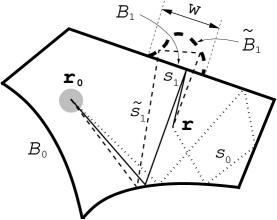
Figure 1: An unperturbed, chaotic billiard (solid-line), together with the perturbation (dashed-line). The boundary of the unperturbed billiard consists of two segments, $\mathcal{B}_{0}$ and $\mathcal{B}_{1}$. The perturbation replaces the latter segment by $\tilde{\mathcal{B}}_{1}$, rendering the perturbed billiard to be bounded by $\mathcal{B}_{0}$ and $\tilde{\mathcal{B}}_{1}$. The initial Gaussian wave packet is centered at ${\bf{r}}_{0}$. Three possible types of trajectories, $s_{0}$, $s_{1}$ and $\tilde{s}_{1}$, leading from ${\bf{r}}_{0}$ to another point ${\bf{r}}$, are shown.

We proceed by considering a Gaussian wave packet,

$$\phi_{0}({\bf{r}})=\frac{1}{\sqrt{\pi}\sigma}\exp\left[\frac{i}{\hbar}\>{\bf{p}}_{0}\cdot({\bf{r}}-{\bf{r}}_{0})-\frac{({\bf{r}}-{\bf{r}}_{0})^{2}}{2\sigma^{2}}\right],$$ (2)

centered at a point ${\bf{r}}_{0}$ inside the domain $\mathcal{A}$ of a two-dimensional chaotic billiard (e.g. the solid-line boundary in Fig. 1), and characterized by an average momentum ${\bf{p}}_{0}$ that defines the de Broglie wavelength of the moving particle, $\lambdabar=\hbar/|{\bf{p}}_{0}|$. The dispersion $\sigma$ is assumed to be sufficiently small for the normalization integral $\int_{\mathcal{A}}d{\bf{r}}|\phi_{0}({\bf{r}})|^{2}$ to be close to unity. We let the wave packet evolve inside the billiard through a time $t$ according to the time-dependent Schrödinger equation with hard-wall (Dirichlet) boundary conditions. This evolution yields the wave function $\phi_{t}({\bf{r}})=\langle{\bf{r}}|e^{-iHt/\hbar}|\phi_{0}\rangle$, where $H$ stands for the Hamiltonian of the billiard. Then, we consider a perturbed billiard obtained from the original one by modifying the shape of a small segment of its boundary. Fig. 1 illustrates the perturbation: the unperturbed billiard is bounded by segments $\mathcal{B}_{0}$ and $\mathcal{B}_{1}$, whereas the boundary of the perturbed billiard is composed of $\mathcal{B}_{0}$ and $\tilde{\mathcal{B}}_{1}$. The perturbation, $\mathcal{B}_{1}\to\tilde{\mathcal{B}}_{1}$, is assumed to be such that the domain $\tilde{\mathcal{A}}$ of the perturbed billiard entirely contains the domain $\mathcal{A}$ of the unperturbed one. The time evolution of the initial wave packet, Eq. (2), inside the perturbed billiard results to $\tilde{\phi}_{t}({\bf{r}})=\langle{\bf{r}}|e^{-i\tilde{H}t/\hbar}|\phi_{0}\rangle$, with $\tilde{H}$ being the Hamiltonian of the perturbed billiard. Then, the LE, defined in Eq. (1), reads

$$M(t)=\left|\int_{\mathcal{A}}d{\bf{r}}\tilde{\phi}_{t}^{*}({\bf{r}})\phi_{t}({\bf{r}})\right|^{2},$$ (3)

where the asterisk denotes complex conjugation.

We now present a semiclassical calculation of the overlap integral Eq. (3). As the starting point we take the expression jalab ; cucch-3 for the time evolution of the small (such that $\sigma$ is much smaller than the characteristic length scale of the billiard) Gaussian wave packet, defined by Eq. (2):

$$\phi_{t}({\bf{r}})\approx(4\pi\sigma^{2})^{1/2}\sum_{s({\bf{r}},{\bf{r}}_{0},\,t)}\!\mathcal{K}_{s}({\bf{r}},{\bf{r}}_{0},t)\>e^{-\sigma^{2}({\bf{p}}_{s}-{\bf{p}}_{0})^{2}/{2\hbar^{2}}}.$$ (4)

This expression is obtained by applying the semiclassical Van Vleck propagator brack , with the action linearized in the vicinity of the wave packet center ${\bf{r}}_{0}$, to the wave packet $\phi_{0}({\bf{r}})$. Here, the sum goes over all possible trajectories $s({\bf{r}},{\bf{r}}_{0},t)$ of a classical particle inside the unperturbed billiard leading from the point ${\bf{r}}_{0}$ to the point ${\bf{r}}$ in time $t$ (e.g. trajectories $s_{0}$ and $s_{1}$ in Fig. 1), and

$$\mathcal{K}_{s}({\bf{r}},{\bf{r}}_{0},t)=\frac{\sqrt{D_{s}}}{2\pi i\hbar}\exp\left(\frac{i}{\hbar}S_{s}({\bf{r}},{\bf{r}}_{0},t)-i\frac{\pi\nu_{s}}{2}\right),$$ (5)

where $S_{s}({\bf{r}},{\bf{r}}_{0},t)$ denotes the classical action along the path $s$. In a hard-wall billiard $S_{s}({\bf{r}},{\bf{r}}_{0},t)=(m/2t)L_{s}^{2}({\bf{r}},{\bf{r}}_{0})$, where $L_{s}({\bf{r}},{\bf{r}}_{0})$ is the length of the trajectory $s$, and $m$ is the mass of the moving particle. In Eq. (5), $D_{s}=|\det(-\partial^{2}S_{s}/\partial{\bf{r}}\partial{\bf{r}}_{0})|$ is the Van Vleck determinant, and $\nu_{s}$ is an index equal to twice the number of collisions with the hard-wall billiard boundary that a particle, traveling along $s$, experiences during time $t$ gasp . In Eq. (4), ${\bf{p}}_{s}=-\partial S_{s}({\bf{r}},{\bf{r}}_{0},t)/\partial{\bf{r}}_{0}$ stands for the initial momentum of a particle on the trajectory $s$. The expression for the time-dependent wave function $\tilde{\phi}_{t}({\bf{r}})$ is obtained from Eq. (4) by replacing the trajectories $s({\bf{r}},{\bf{r}}_{0},t)$ by paths $\tilde{s}({\bf{r}},{\bf{r}}_{0},t)$, that lead from ${\bf{r}}_{0}$ to ${\bf{r}}$ in time $t$ within the boundaries of the perturbed billiard (e.g. trajectories $s_{0}$ and $\tilde{s}_{1}$ in Fig. 1).

The wave functions of the unperturbed and perturbed billiards at a point ${\bf{r}}\in\mathcal{A}$ can be written as

$$\begin{split}\phi_{t}({\bf{r}})&=\phi_{t}^{(0)}({\bf{r}})+\phi_{t}^{(1)}({\bf{r}}),\\ \tilde{\phi}_{t}({\bf{r}})&=\phi_{t}^{(0)}({\bf{r}})+\tilde{\phi}_{t}^{(1)}({\bf{r}}),\end{split}$$ (6)

where $\phi_{t}^{(0)}({\bf{r}})$ is given by Eq. (4) with the sum in the RHS involving only trajectories $s_{0}$, which scatter only off the part of the boundary, $\mathcal{B}_{0}$, that stays unaffected by the perturbation, see Fig. 1. On the other hand, the wave function $\phi_{t}^{(1)}$ ( $\tilde{\phi}_{t}^{(1)}$ ) involves only such trajectories $s_{1}$ ( $\tilde{s}_{1}$ ) that undergo at least one collision with the perturbation-affected region, $\mathcal{B}_{1}$ ( $\tilde{\mathcal{B}}_{1}$ ), see Fig. 1. The LE integral in Eq. (3) has now four contributions:

$$\begin{split}\int_{\mathcal{A}}d{\bf{r}}\tilde{\phi}_{t}^{*}\phi_{t}&=\int_{\mathcal{A}}d{\bf{r}}\left|\phi_{t}^{(0)}\right|^{2}+\int_{\mathcal{A}}d{\bf{r}}\left[\phi_{t}^{(0)}\right]^{*}\phi_{t}^{(1)}\\ &+\int_{\mathcal{A}}d{\bf{r}}\left[\tilde{\phi}_{t}^{(1)}\right]^{*}\phi_{t}^{(0)}+\int_{\mathcal{A}}d{\bf{r}}\left[\tilde{\phi}_{t}^{(1)}\right]^{*}\phi_{t}^{(1)}.\end{split}$$ (7)

We argue that the dominant contribution to the LE overlap comes from the first integral in the RHS of the last equation. Indeed, all the integrands in Eq. (7) contain the factor $\exp[i(S_{s}-S_{s^{\prime}})/\hbar-i\pi(\nu_{s}-\nu_{s^{\prime}})/2]$, where the trajectory $s$ is either of the type $s_{0}$ or $s_{1}$, and $s^{\prime}$ is either of the type $s_{0}$ or $\tilde{s}_{1}$, see Fig. 1. An integral vanishes if there is no correlation between $s$ and $s^{\prime}$, since the corresponding integrand is a rapidly oscillating function of ${\bf{r}}$. This is indeed the case for the last two integrals: they involve such trajectory pairs $(s,s^{\prime})$ that $s$ is of the type $s_{0}$ or $s_{1}$, and $s^{\prime}$ is of the type $\tilde{s}_{1}$, so that the absence of correlations within such pairs is guaranteed by the fact that the scale of the boundary deformation is much larger than $\lambdabar$. Then, we restrict ourselves to the diagonal approximation, in which only the trajectory pairs with $s=s^{\prime}$ survive the integration over ${\bf{r}}$. The second integral in the RHS of Eq. (7) only contains the trajectory pairs of the type $(s_{0},s_{1})$, and, therefore, vanishes in the diagonal approximation. Thus, the only non-vanishing contribution reads

$$\begin{split}\int_{\mathcal{A}}d{\bf{r}}\left|\phi_{t}^{(0)}\right|^{2}&\approx\frac{\sigma^{2}}{\pi\hbar^{2}}\int_{\mathcal{A}}d{\bf{r}}\sum_{s_{0}}D_{s_{0}}\exp\left[-\frac{\sigma^{2}}{\hbar^{2}}\left({\bf{p}}_{s_{0}}-{\bf{p}}_{0}\right)^{2}\right]\\ &\approx\int_{\mathcal{P}_{t}(\mathcal{A})}d{\bf{p}}\>\frac{\sigma^{2}}{\pi\hbar^{2}}\exp\left[-\frac{\sigma^{2}}{\hbar^{2}}\left({\bf{p}}-{\bf{p}}_{0}\right)^{2}\right],\end{split}$$ (8)

where $D_{s_{0}}=|\det(\partial{\bf{p}}_{s_{0}}/\partial{\bf{r}})|$, with ${\bf{p}}_{s_{0}}$ being the initial momentum on the trajectory $s_{0}({\bf{r}},{\bf{r}}_{0},t)$, serves as the Jacobian of the transformation from the space of final positions ${\bf{r}}\in\mathcal{A}$ to the space of initial momenta ${\bf{p}}\in\mathcal{P}_{t}(\mathcal{A})$. Here, $\mathcal{P}_{t}(\mathcal{A})$ is the set of all momenta ${\bf{p}}$ such that a trajectory, starting from the phase-space point $({\bf{r}}_{0},{\bf{p}})$, arrives at a coordinate point ${\bf{r}}\in\mathcal{A}$ after the time $t$, while undergoing collisions only with the boundary $\mathcal{B}_{0}$ (and, thus, avoiding $\mathcal{B}_{1}$), see Fig. 1. Thus, $\int_{\mathcal{A}}d{\bf{r}}|\phi_{t}^{(0)}|^{2}$ is merely the probability that a classical particle, with the initial momentum sampled from the Gaussian distribution, experiences no collisions with $\mathcal{B}_{1}$ during the time $t$. Therefore, if the boundary segment $\mathcal{B}_{1}$ is removed, this integral corresponds to the survival probability of the classical particle in the resulting open billiard. In chaotic billiards the survival probability decays exponentially bauer as $e^{-\gamma t}$, with the escape rate $\gamma$ given by

$$\gamma=v\frac{w}{\pi A},$$ (9)

where $v=|{\bf{p}}_{0}|/m$ is the particle’s velocity, and $A$ stands for the area of the billiard. Equation (9) assumes that the characteristic escape time $1/\gamma$ is much longer that the average free flight time $t_{\mathrm{f}}$. In chaotic billiards the latter is given by niels $t_{f}=\pi A/vP$, where $P$ is the perimeter of the billiard. Condition $t_{\mathrm{f}}\ll 1/\gamma$ is equivalent to $w\ll P$.

In accordance with Eqs. (3) and (7) the LE decays as

$$M(t)\sim\exp(-2\gamma t).$$ (10)

Equation (10) constitutes the central result of the paper. Together with Eq. (9) it shows that for a given billiard the LE merely depends on the length $w$ of the boundary segment affected by the perturbation and on the de Broglie wavelength $\lambdabar=\hbar/mv$. It is independent of the shape and area of the boundary perturbation, as well as of the position, size and momentum direction of the initial wave packet. (We exclude initial conditions for which the wave packet interacts with the perturbation before having considerably explored the allowed phase space.)

The decay rate $\gamma$, and thus the LE, are also related to classical properties of the chaotic set of periodic trajectories unaffected by the boundary perturbation, i.e. to properties of the chaotic repellor of the open billiard kantz :

$$\gamma=\lambda_{\mathrm{r}}-h_{\mathrm{KS}},$$ (11)

where $\lambda_{\mathrm{r}}$ is the average Lyapunov exponent of the repellor, and $h_{\mathrm{KS}}$ is its Kolmogorov-Sinai entropy. Thus, Eqs. (10) and (11) provide an interesting link between classical and quantum chaos.

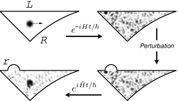
Figure 2: Forward-time wave packet evolution in the unperturbed DD billiard, followed by the reversed-time evolution in the perturbed billiard. The initial Gaussian wave packet is characterized by the size $\sigma=12$ and de Broglie wavelength $\lambdabar=15/\pi$; the arrow shows the momentum direction of the initial wave packet. The DD billiard is characterized by $L=400$ and $R=200\sqrt{10}$. The perturbation is defined by $w=60$ and $r=30$. The propagation time corresponds to approximately 10 collisions of the classical particle.

In order to verify the analytical predictions we simulated the dynamics of a Gaussian wave packet inside a desymmetrized diamond (DD) billiard, defined as the fundamental domain of the area confined by four intersecting disks centered at the vertices of a square. According to the theorem of Ref. szasz the DD billiard is chaotic in the classical limit. It can be characterized by the disk radius $R$, and the length $L$ of the longest straight segment of the boundary, see Fig. 2. We consider the Hamiltonian perturbation that replaces a straight segment of length $w$ of the boundary of the unperturbed billiard by an arc of radius $r$, see Fig. 2. In general, $w\leq 2r$.

To simulate the time evolution of the wave packet inside the billiard we utilize the Trotter-Suzuki algorithm raedt . Figure 2 illustrates the time evolution of a Gaussian wave packet in the DD billiard followed by the time-reversed evolution inside the perturbed billiard. The parameters characterizing the system are $L=400$, $R=200\sqrt{10}$, $w=60$ and $r=30$. The Gaussian wave packet is parametrized by $\sigma=12$, $\lambdabar=15/\pi$; the arrow shows the momentum direction of the initial wave packet. The evolution time $t$ in Fig. 2 corresponds to some 10 free flight times of the corresponding classical particle, i.e. $t=10t_{\mathrm{f}}$.

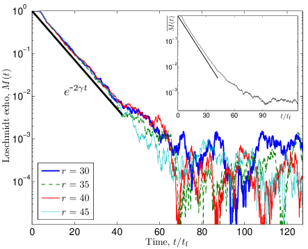
Figure 3: (Color online) The Loschmidt echo (LE) decay in the DD billiard for four different values of the curvature radius $r$ of the arc perturbation. The width of the perturbation region is fixed, $w=60$. The other system parameters are $L=400$, $R=200\sqrt{10}$, $\sigma=3$, and $\lambdabar=5/\pi$. The solid straight line gives the trend of the $\exp(-2\gamma t)$ decay, with $\gamma$ given by Eq. (9). The inset presents the decay of the average LE, with averaging performed over individual LE curves corresponding to different values of $r$.

Figure 3 shows the time dependence of the LE computed for the DD billiard system characterized by $L=400$, $R=200\sqrt{10}$, $\sigma=3$, and $\lambdabar=5/\pi$. The initial momentum direction is the same as in Fig. 2. The different LE decay curves correspond to different shapes of the local boundary perturbation: the width of the perturbation region stays fixed, $w=60$, and the curvature radius of the perturbation arc takes the values $r=30;\,35;\,40;\,45$. In all four cases the LE displays the exponential decay for times $t$ up to 40$t_{\mathrm{f}}$-45$t_{\mathrm{f}}$ followed by LE fluctuations around a saturation value, $M_{\mathrm{s}}$. The thick solid straight line shows the trend of the $e^{-2\gamma t}$ exponential decay, with $\gamma$ given by Eq. (9). One can see strong agreement between the numerical and analytical LE decay rates. We have also verified numerically that the LE decay rate is independent of the momentum direction of the initial wave packet.

The inset in Fig. 3 presents the time decay of the average LE $\overline{M(t)}$, with the averaging performed over 16 individual decay curves $M(t)$ corresponding to different values of the arc radius $r$, ranging from $r=30$ to $45$. The saturation mechanism for the LE decay was first proposed by Peres peres and later discussed in Ref. cucch-3 . The LE saturates at a value $M_{\mathrm{s}}$ inversely proportional to the number $N$ of energy levels significantly represented in the initial state. If the areas of the unperturbed and perturbed billiards are relatively close, then $N\approx A/\sigma^{2}$ and $M_{\mathrm{s}}\sim\sigma^{2}/A$. (We have verified the latter relation by computing the LE saturation value for billiards of different area.) Thus, one might expect the exponential decay of the LE to persist for times $t\lesssim t_{\mathrm{s}}$, with the saturation time $t_{\mathrm{s}}=(1/2\gamma v)\ln N$. The latter can be longer than the Heisenberg time $t_{\mathrm{H}}=A/2\pi\lambdabar v$ for a system with sufficiently large effective Hilbert space, since $t_{\mathrm{s}}/t_{\mathrm{H}}\sim(\lambdabar/w)\ln N$. Indeed, for the system corresponding to Fig. 3 one has $t_{\mathrm{H}}\approx 29t_{\mathrm{f}}$, whereas the exponential decay persists for times $t<40t_{\mathrm{f}}$.

Finally, we sketch a principal experimental scheme for measuring the LE decay regime proposed in this paper. Consider a two-dimensional, AlGaAs-GaAs heterojunction-based ballistic cavity with the shape of a chaotic billiard, e.g. Fig. 1. Let the initial electron state to be given by $|\Psi_{0}\rangle=|\phi_{0}\rangle\otimes|\chi\rangle$, where $|\phi_{0}\rangle$ is the spatial part defined by Eq. (2), and $|\chi\rangle=2^{-1/2}\left(|\!\uparrow\rangle+|\!\downarrow\rangle\right)$ represents a spin-1/2 state. Here, $|\!\uparrow\rangle$ and $|\!\downarrow\rangle$ are the eigenstates of the spin-projection operator in the $z$-direction, perpendicular to the billiard plane. Then, $|\chi\rangle$ is the eigenstate of the spin-projection operator $s_{x}=\frac{\hbar}{2}\sigma_{x}$, with $\sigma_{x}=|\!\uparrow\rangle\langle\downarrow\!|+|\!\downarrow\rangle\langle\uparrow\!|$, in some $x$-direction, fixed in the billiard plane. Suppose now that a half-metallic ferromagnet, magnetized in the $z$-direction, is attached to the boundary of the ballistic cavity. (One may consider the region bounded by $\mathcal{B}_{0}$ and $\mathcal{B}_{1}$ in Fig. 1 to represent the ballistic cavity, and the region bounded by $\mathcal{B}_{1}$ and $\tilde{\mathcal{B}}_{1}$ to represent the ferromagnet.) Then the ferromagnet-cavity interface will reflect the $|\!\uparrow\rangle$-component of the state, but will transmit the $|\!\downarrow\rangle$-component. As a result, the two components will evolve under two different spatial Hamiltonians, $H$ and $\tilde{H}$, corresponding to the geometry of the ballistic cavity and the geometry of the cavity-ferromagnet compound respectively. Then $|\Psi_{0}\rangle$ will evolve to

$$|\Psi_{t}\rangle=\frac{1}{\sqrt{2}}\left[e^{-iHt/\hbar}|\phi_{0}\rangle\otimes|\!\uparrow\rangle+e^{-i\tilde{H}t/\hbar}|\phi_{0}\rangle\otimes|\!\downarrow\rangle\right].$$ (12)

The expectation value of the projection of the spin in the $x$-direction is related to the LE overlap by

$$\bar{s}_{x}(t)\equiv\langle\Psi_{t}|s_{x}|\Psi_{t}\rangle=\frac{\hbar}{2}\mathrm{Re}\langle\phi_{0}|e^{i\tilde{H}t/\hbar}e^{-iHt/\hbar}|\phi_{0}\rangle,$$ (13)

where $\mathrm{Re}$ denotes the real part. As we have shown above, this overlap is real and decays exponentially in time. Therefore, the average spin projection in the $x$-direction will also relax exponentially with time, i.e. $\bar{s}_{x}(t)\sim\frac{\hbar}{2}\exp(-\gamma t)$, with the relaxation rate $\gamma$ determined by Eq. (9). This result provides a link between the spin relaxation in chaotic, mesoscopic structures been and the LE decay due to local boundary perturbations.

The authors would like to thank Inanc Adagideli, Arnd Bäcker, Fernando Cucchietti, Philippe Jacquod, Thomas Seligman, and Oleg Zaitsev for helpful conversations. AG acknowledges the Alexander von Humboldt Foundation (Germany), and KR acknowledges the Deutsche Forschungsgemeinschaft (DFG) for support of the project.

References

- (1) A. Peres, Phys. Rev. A 30, 1610 (1984).
- (2) see, e.g., T. Gorin, T. Prosen, T. H. Seligman, and M. Znidaric, Phys. Rep. 435, 33 (2006); C. Petitjean and Ph. Jacquod, Phys. Rev. E 71, 036223 (2005), and references therein.
- (3) R. A. Jalabert and H. M. Pastawski, Phys. Rev. Lett. 86, 2490 (2001).
- (4) F. M. Cucchietti, H. M. Pastawski, and R. A. Jalabert, Phys. Rev. B 70, 035311 (2004).
- (5) M. Brack and R. K. Bhaduri, Semiclassical physics, Frontier in Physics, Vol. 96, (Westview Press, Boulder, 1997).
- (6) P. Gaspard and S. A. Rice, J. Chem Phys. 90, 2242 (1989).
- (7) see, e.g., O. Legrand and D. Sornette, Phys. Rev. Lett. 66, 2172 (1991), and references therein.
- (8) S. F. Nielsen, P. Dahlqvist, and P. Cvitanović, J. Phys. A 32, 6757 (1999).
- (9) H. Kantz and P. Grassberger, Physica D 17, 75 (1985); J.-P. Eckmann and D. Ruelle, Rev. Mod. Phys. 57, 617 (1985).
- (10) A. Krámli, N. Simányi, and D. Szász, Comm. Math. Phys. 125, 439 (1989).
- (11) H. De Raedt, Annu. Rev. Comput. Phys. 4, 107 (1996).
- (12) C. W. J. Beenakker, Phys. Rev. B 73, 201304(R) (2006).