Comparative Study of Different Discretizations of the $\phi^{4}$ Model

Abstract

We examine various recently proposed discretizations of the well-known $\phi^{4}$ field theory. We compare and contrast the properties of their fundamental solutions including the nature of their kink-type solitary waves and the spectral properties of the linearization around such waves. We study these features as a function of the lattice spacing $h$, as one deviates from the continuum limit of $h\rightarrow 0$. We then proceed to a more “stringent” comparison of the models, by discussing the scattering properties of a kink-antikink pair for the different discretizations. These collisions are well-known to possess properties that quite sensitively depend on the initial speed even at the continuum limit. We examine how typical model behaviors are modified in the presence (and as a function) of discreteness and attempt to extract qualitative trends and issue pertinent warnings about some of the surprising resulting properties.

I Introduction

In the past few years, a variety of physical applications ranging from Bose-Einstein condensates in optical lattices konotop , to arrays of waveguides in nonlinear optics nlo and even to the dynamics of DNA peyrard have stimulated an enormous growth in the study of discrete models and the differential-difference equations that describe them. These models have a two-fold role and importance. On the one hand, they serve as discretizations of the corresponding continuum field theories; however, on the other hand, they may also be important physical models in their own right, e.g. in the context of crystal lattices.

An important class of models (and discretizations thereof) that is relevant to a wide variety of applications consists of the so-called Klein-Gordon type equations kivshar1 . One of the particularly interesting equations within this family is the so-called $\phi^{4}$ model belova , featuring a wave equation with a cubic nonlinear (odd-power) polynomial added to it. This model has been physically argued as being of relevance in describing cosmic domain walls in cosmological settings anninos , but also structural phase transitions, uniaxial ferroelectrics or even simple polymeric chains; see e.g. Campbell and references therein. A particularly intriguing feature that was discovered early on in the continuum limit was the existence of a fractal structure anninos in the collisions between the fundamental nonlinear wave structures (a kink and an anti-kink) in this model. This is a topic that was initiated by the numerical investigations of Refs. Campbell ; Campbell1 (see also belova ) and is a topic that is still under active investigation (see e.g., the very recent mathematical analysis of the relevant mechanism provided in Ref. goodman ).

On the other hand, more recently, an issue that has concerned research work has been how to produce discretizations of such continuum models (such as the $\phi^{4}$ model or its complex cousin, the nonlinear-Schrödinger equation sulem ) that preserve some of the important properties of the corresponding continuum limit. One of the non-trivial aspects of this endeavor is the generation of discrete models in space that maintain some of the key invariances of their continuum siblings. For instance, in the uniform continuum medium, solutions can be shifted arbitrarily along a certain direction $x$ by any $x_{0}$ ($x$ is the spatial coordinate and $x_{0}={\rm const.}$), due to the underlying translational invariance. However, discretizations generically will fail to maintain that feature and in the most straightforward versions thereof, equilibrium static solutions exist for a discrete rather than a continuum set of $x_{0}$ kivshar1 . Some of these equilibrium solutions correspond to energy maxima and are unstable, while others, corresponding to energy minima, are stable. The difference between such maxima and minima of the energy is typically referred to as the Peierls-Nabarro barrier (PNb). One of the topics of intense research efforts in the past few years has been to develop discretizations that do not present such energetic barriers; this is done in the hope that the latter class of models may provide more faithful representations of their continuum counterparts, regarding both symmetry properties and traveling solution features.

The result of the above considerations in recent years has been the systematic construction of a large class of non-integrable discrete Klein-Gordon equations free of the Peierls-Nabarro barrier (PNb-free). Since the standard discretization of the continuum $\phi^{4}$ models conserves the energy but does have a PNb, Speight and co-workers SpeightKleinGordon (see also Speight ; SpeightPhi4 ) originally used a Bogomol’nyi argument Bogom , in order to eliminate that barrier. A later successful attempt (that produced multiple PNb-free models) was based on a different perspective, namely the one of associating the PNb-free models to momentum-conserving discretizations KevrekidisPhysD . Subsequently, yet another such model was recently proposed in Saxena . Furthermore, these approaches were systematized and generalized through their formulation by means of a two-point discrete version of the first integral of the static continuum Klein-Gordon equation JPhysA ; Barashenkov . We should note in passing that similar discretization efforts have recently been extended to the nonlinear Schrödinger equation dk ; dep ; krss .

One of the important questions that naturally emerges in the presence of this extensive recent literature is, indeed, how accurately do we expect these models to track the continuum limit behavior and how various properties are affected by the discreteness, as a function of its characteristic parameter (the lattice spacing $h$). Already, to some extent, there have been concerns regarding that question in that simulations of more sensitive phenomena such as kink collisions in the “Speight discretization” SpeightKleinGordon ; SpeightPhi4 were only faithful to the continuum limit for fine lattices ($h\approx 0.1$ or less) almeida . Here, we examine this question a bit more broadly and in more detail through numerical computations and analytical considerations comparing/contrasting five different discretizations of the continuum $\phi^{4}$ field theory. Among them is the “standard”, classical $\phi^{4}$ discretization (Model 1) Campbell , two energy-conserving discretizations, namely the Speight-one (Model 2) SpeightKleinGordon and the one of Ref. Saxena also labeled CKMS hereafter (Model 3), and two momentum-conserving discretizations stemming from Ref. KevrekidisPhysD , labeled K1 (Model 4) and K2 (Model 5), respectively. For each one of these models, we begin by examining the properties of the fundamental building block nonlinear wave solutions, namely the discrete kinks (and antikinks). We show how to obtain such solutions analytically or semi-analytically and subsequently examine the spectrum of small-amplitude excitations (linearization) around them, among other properties (such as stability) because this spectrum plays a nontrivial role in the outcome of wave interactions. Finally, we focus on the latter (i.e., on solitary wave collisions between kinks and antikinks) and attempt to extract salient features of such interactions as a function of the lattice spacing $h$ and for a set of different speeds (and also different initial separations between the kinks).

Our main findings can be summarized as follows:

• The different models yield kink profiles that are different between them and from the continuum limit. These differences are strongest for the CKMS model and are found to lead to shrinking kinks for the energy conserving models 1-3, while they lead to expanding kinks in models 4-5. The deviation from the relevant continuum profile grows as $h^{2}$.

• The boosting of the kinks in order to induce their collision excites their internal modes. This plays a significant role in the collisions, since for different initial distances, the excitation of the internal mode will carry a different phase (at the moment of collision) and may accordingly lead to different collision outcomes.

• The different models have different properties as regards the elasticity of their collisions. The most inelastic collisions occur in the standard discretization of model 1. Perhaps the next least elastic collisions occur in the CKMS Model 3, then K1 (Model 4), Speight (Model 2) and K2 (Model 5) in order of increasing elasticity.

• The elasticity of collisions changes as a function of the lattice spacing. In fact, remarkably so, the collisions are more elastic for larger values of the lattice spacing. This is also demonstrated in the decreasing dependence of the critical velocity (beyond which the solitary waves separate after one collision) as a function of $h$.

The presentation of our results will be structured as follows. In section II, we will present the various models and, in section III, compare their kink solutions and spectral properties. In section IV, we will examine the properties of the collisions of the different models focusing on a few typical speeds of the incoming waves for different initial distances and for different initial lattice spacings. Finally, in section V, we will summarize our findings and present our conclusions, as well as some open questions for future study.

II $\phi^{4}$ field and its various discretizations

Starting from the continuum limit of the model, we note that the one-dimensional $\phi^{4}$ field is described by the Lagrangian ${\cal L}=E_{K}-E_{P}$ with the kinetic and potential energy functionals defined, respectively, by

$$E_{K}=\frac{1}{2}\int_{-\infty}^{\infty}\phi_{t}^{2}dx\,,$$ (1)

$$E_{P}=\frac{1}{2}\int_{-\infty}^{\infty}\left[\phi_{x}^{2}+\left(1-\phi^{2}\right)^{2}\right]dx\,,$$ (2)

where $\phi(x,t)$ is the scalar field of interest and subscript indices mean partial derivatives with respect to the corresponding variable. The resulting Euler-Lagrange equation is obtained by demanding that $\phi$ be a local extremum of the action $S=\int{\cal L}{\rm d}t$, and it reads

$$\phi_{tt}=\phi_{xx}+2\phi(1-\phi^{2})\,.$$ (3)

The following kink (antikink) solution to Eq. (3),

$$\phi(x,t)=\pm\tanh\frac{x-x_{0}-vt}{\sqrt{1-v^{2}}},$$ (4)

is one of the simplest examples of topological solitons. In Eq. (4), $v$ is the kink velocity and $x_{0}$ is its arbitrary initial position (signalling the translational invariance of the continuum model discussed in the previous section).

The first integral of the static version of Eq. (3),

$$U(x)\equiv\phi_{x}^{2}-(1-\phi^{2})^{2}=0\,,$$ (5)

plays an important role in our considerations. The integration constant was set to zero in Eq. (5), which is sufficient for obtaining the kink solutions. The first integral can also be taken in a modified form, e.g., as

$$u(x)\equiv\pm\phi_{x}-1+\phi^{2}=0\,.$$ (6)

We study various lattice dynamical equations obtained by discretizing Eq. (3) on the lattice $x=nh$, where $n=0,\pm 1,\pm 2...$, and $h$ is the lattice spacing. The general form of the lattice equations studied herein is

$$\ddot{\phi}_{n} = \Delta_{2}\phi_{n}+F(\phi_{n-1},\phi_{n},\phi_{n+1})$$ (7)

$$\equiv D(\phi_{n-1},\phi_{n},\phi_{n+1}),$$

where

$$\Delta_{2}\phi_{n}=\frac{1}{h^{2}}(\phi_{n-1}-2\phi_{n}+\phi_{n+1}),$$ (8)

and, in the continuum limit $(h\rightarrow 0)$,

$$F(\phi_{n-1},\phi_{n},\phi_{n+1})\rightarrow 2\phi(1-\phi^{2}).$$ (9)

As mentioned previously, of particular interest will be the lattices whose static solutions, satisfying the three-point static problem corresponding to Eq. (7),

$$D(\phi_{n-1},\phi_{n},\phi_{n+1})=0,$$ (10)

can be found from a reduced two-point problem of the form

$$U(\phi_{n-1},\phi_{n})=0,$$ (11)

or of the form

$$u(\phi_{n-1},\phi_{n})=0.$$ (12)

Equations (11) and (12) are the discretized first integrals (DFIs) obtained by discretizing Eq. (5) and Eq. (6), respectively JPhysA (see also Barashenkov ).

Lattices whose static solutions can be found from the two-point DFI are called translationally invariant because the equilibrium solution can be obtained iteratively from the nonlinear algebraic equation starting from an arbitrary admissible value $\phi_{n}$. In other words, translationally invariant lattices support a continuum rather than a discrete set of equilibrium solutions parametrized, e.g., by the position of the $n$th particle, $\phi_{n}$.

Let us now calculate the PN barrier in the models whose static solutions can be found from a two-point DFI, i.e., in the translationally invariant lattices. We consider a continuum set of equilibrium solutions parameterized by the position of the $n$th particle, $\phi_{n}$, in the range $\phi_{n}\in[\phi_{n}^{(1)},\phi_{n}^{(2)}]$, assuming that all values of $\phi_{n}$ within this range are admissible.

The work done by the inter-particle and the background forces (originating from the discretized background potential) to move (quasi-statically) the $n$th particle from the configuration $\phi^{(1)}$ to the configuration $\phi^{(2)}$ is

$$W_{n}=\int_{\phi_{n}^{(1)}}^{\phi_{n}^{(2)}}D(\phi_{n-1},\phi_{n},\phi_{n+1}){\rm d}\phi_{n},$$ (13)

and the total work performed to “transform” the whole chain from $\phi^{(1)}$ to $\phi^{(2)}$ is

$$W=\sum_{n=-\infty}^{\infty}W_{n}.$$ (14)

However, in the translationally invariant models, the availability of a path of equilibrium configurations allowing to transit from $\phi^{(1)}$ to $\phi^{(2)}$ leads to $D=0$ and thus, $W_{n}=0$ for all $n$. This, in turn, results in $W=0$. This result suggests that there is no energy cost to transform quasi-statically one equilibrium solution into another through a continuous set of equilibrium solutions. In other words, the height of the Peierls-Nabarro barrier calculated along this path is zero. For Hamiltonian lattices, the total work is path-independent (and equal to the potential energy difference between the final and initial state) and we can claim that, in such dynamical lattices, the PN potential is zero. For non-Hamiltonian lattices the work is path-dependent and we can only claim the absence of the PN barrier along the path considered above (which, however, is a natural one). While there are mathematical subtleties as regards whether this notion yields zero PNb more generally for translationally invariant lattices, this is the definition of PNb-free models that will be used herein. A more detailed examination of the, admittedly interesting, pertinent topics is outside the scope of the present study focusing on the comparison between different discrete $\phi^{4}$ models and will be delegated to a future publication.

In the following, we consider various discrete $\phi^{4}$ models reported in the literature describing their kink solutions, their spectra of small-amplitude vibrations around vacuum solutions ($\phi_{n}=\pm 1$), and also the spectra of lattices containing one static kink, revealing the kink’s internal vibrational modes. Physical quantities conserved by the lattices are given, if they exist. These results will be quite relevant also in the discussion of kink-antikink collision outcomes.

II.1 Classical discretization (model 1)

The “standard” discretization of Eq. (3) is Campbell

$$\ddot{\phi}_{n}=\Delta_{2}\phi_{n}+2\phi_{n}(1-\phi_{n}^{2}),$$ (15)

and this is the only lattice in this study that possesses a Peierls-Nabarro barrier.

Model 1 conserves the Hamiltonian (total energy)

$$H_{1}=\frac{h}{2}\sum_{n}\left[\dot{\phi}_{n}^{2}+\frac{\left(\phi_{n+1}-\phi_{n}\right)^{2}}{h^{2}}+\left(1-\phi_{n}^{2}\right)^{2}\right].$$ (16)

Static kink solutions in model 1 exist only for those waves centered at a lattice site (unstable) or in the middle between two neighboring lattice sites (stable). Solutions can be found by various numerical techniques. As a first approximation, one can adopt Eq. (4) to write the following approximate static kink solution

$$\phi_{n}=\pm\tanh[h(n-x_{0})].$$ (17)

One can use this ansatz in a fixed point scheme (such as a Newton method) for $x_{0}=0$ or $x_{0}=1/2$ (mod 1), to identify the exact discrete static solutions $\phi_{n}^{0}$.

Subsequently, introducing the ansatz $\phi_{n}(t)=\phi_{n}^{0}+\varepsilon_{n}(t)$ (where $\phi_{n}^{0}$ is an equilibrium solution and $\varepsilon_{n}(t)$ is a small perturbation), we linearize Eq. (15) with respect to $\varepsilon_{n}$ and obtain the following equation:

$$\ddot{\varepsilon}_{n}=\Delta_{2}\varepsilon_{n}+2\varepsilon_{n}-6(\phi_{n}^{0})^{2}\varepsilon_{n}.$$ (18)

For the small-amplitude phonons, $\varepsilon_{n}=\exp(ikn+i\omega t)$, with frequency $\omega$ and wave number $k$, Eq. (18) is reduced to the following dispersion relation:

$$\omega^{2}=\frac{4}{h^{2}}\sin^{2}\left(\frac{k}{2}\right)-2+6(\phi_{n}^{0})^{2}.$$ (19)

From Eq. (19), the spectrum of the vacuum solution, $\phi_{n}^{0}=\pm 1$, is

$$\omega^{2}=4+\frac{4}{h^{2}}\sin^{2}\left(\frac{k}{2}\right).$$ (20)

The spectrum of the lattice when linearizing around a static kink is shown in Fig. 1.

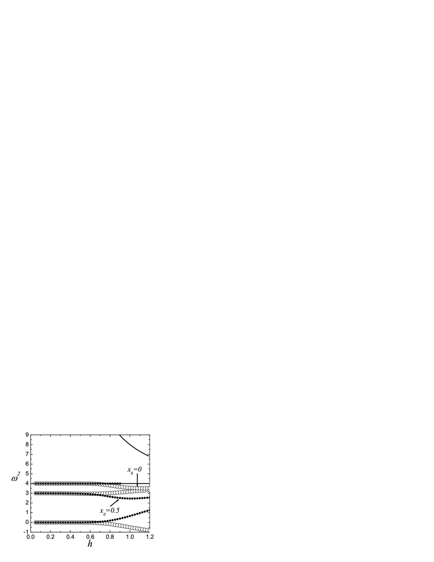
Figure 1: Model 1, Eq. (15): Frequencies of the kink’s internal modes for different magnitudes of the discreteness parameter $h$. Results for the on-site (circles) and inter-site (dots) kinks. Two solid lines show the borders of the spectrum of vacuum, Eq. (20). The on-site kink is unstable because the spectrum contains imaginary frequencies, while the inter-site kink is stable. All three internal models are below the phonon band.

II.2 Energy-conserving model 2

Here we use the following DFI obtained from Eq. (12),

$$u_{2}\equiv\pm\frac{\phi_{n}-\phi_{n-1}}{h}-1+\frac{\phi_{n-1}^{2}+\phi_{n-1}\phi_{n}+\phi_{n}^{2}}{3}=0.$$ (21)

The Hamiltonian, ${\cal H}=E_{K}+E_{P}$, defined by Eq. (1) and Eq. (2), can be discretized as follows,

$$H_{2}=h\sum_{n}\left(\frac{\dot{\phi}_{n}^{2}}{2}+u_{2}^{2}\right),$$ (22)

which gives the equations of motion of the energy-conserving model after Speight SpeightKleinGordon (see also SpeightPhi4 ),

$$\ddot{\phi}_{n} = -u_{2}(\phi_{n-1},\phi_{n})\frac{\partial}{{\partial\phi_{n}}}u_{2}(\phi_{n-1},\phi_{n})-u_{2}(\phi_{n},\phi_{n+1})\frac{\partial}{{\partial\phi_{n}}}u_{2}(\phi_{n},\phi_{n+1})$$ (23)

$$= \left(1+\frac{h^{2}}{3}\right)\Delta_{2}\phi_{n}+2\phi_{n}-\frac{1}{9}\left[2\phi_{n}^{3}+(\phi_{n}+\phi_{n-1})^{3}+(\phi_{n}+\phi_{n+1})^{3}\right].$$

It is clear that the static solutions to Eq. (23) can be found from the two-point problem, Eq. (21). We have

$$\phi_{n\pm 1}=-\frac{\phi_{n}}{2}\mp\frac{3}{2h}\pm\frac{\sqrt{3}}{2}\sqrt{-\phi_{n}^{2}\pm\frac{6}{h}\phi_{n}+\frac{3}{h^{2}}+4},$$ (24)

where one can take either the upper or the lower signs. The kink solution can be obtained iteratively from Eq. (24), starting from any $|\phi_{n}|<1$. For the on-site and inter-site kinks one should take for the initial value $\phi_{n}=0$ and $\phi_{n}=3/h-\sqrt{3+9/h^{2}}$, respectively.

The equation of motion, Eq. (23), linearized in the vicinity of an equilibrium solution $\phi_{n}^{0}$ yields

$$\ddot{\varepsilon}_{n}=\left(1+\frac{h^{2}}{3}\right)\Delta_{2}\varepsilon_{n}+2\varepsilon_{n}-\frac{1}{9}\Big{[}6(\phi_{n}^{0})^{2}\varepsilon_{n}+3(\phi_{n}^{0}+\phi_{n-1}^{0})^{2}(\varepsilon_{n}+\varepsilon_{n-1})+3(\phi_{n}^{0}+\phi_{n+1}^{0})^{2}(\varepsilon_{n}+\varepsilon_{n+1})\Big{]}.$$ (25)

The spectrum of the vacuum solution, $\phi_{n}^{0}=\pm 1$, is

$$\omega^{2}=4+4\frac{1-h^{2}}{h^{2}}\sin^{2}\left(\frac{k}{2}\right).$$ (26)

On the other hand, the spectrum of linearization around a kink is shown in Fig. 2.

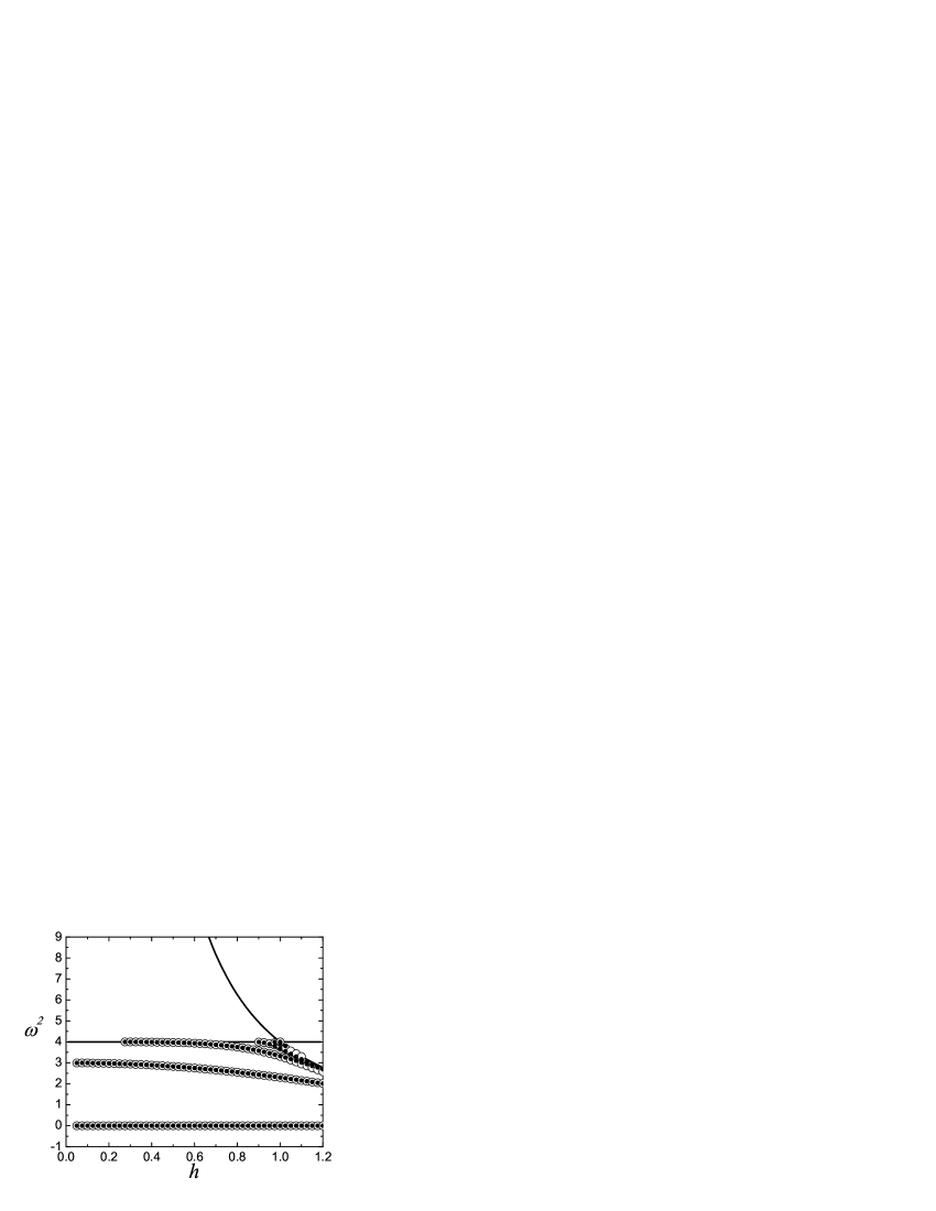
Figure 2: Model 2, Eq. (23). Same as in Fig. 1. Notice the difference of the mode closest to the origin which in this case remains at $\omega^{2}=0$ contrary to what is the case for model 1. There are three internal modes. However, note that a fourth mode appears for $h>0.85$. There is a zero mode for all values of $h$ indicating the absence of a PN barrier.

II.3 Energy-conserving model 3

We take the DFI, corresponding to Eq. (5), in the form

$$U_{3}\equiv\frac{1}{h^{2}}(\phi_{n}-\phi_{n-1})^{2}-(1-\phi_{n-1}\phi_{n})^{2}=0.$$ (27)

The equations of motion of the model of CKMS Saxena ,

$$\ddot{\phi}_{n} = \frac{U_{3}(\phi_{n},\phi_{n+1})-U_{3}(\phi_{n-1},\phi_{n})}{(\phi_{n+1}-\phi_{n-1})(1-h^{2}\phi_{n}^{2})}$$ (28)

$$= \Delta_{2}\phi_{n}+2\frac{\phi_{n}-\phi_{n}^{3}}{1-h^{2}\phi_{n}^{2}},$$

can be obtained from the Hamiltonian

$$H_{3}=\frac{1}{2}\sum_{n}\Big{[}{\dot{\phi}}_{n}^{2}+\frac{(\phi_{n}-\phi_{n-1})^{2}}{h^{2}}+V(\phi_{n})\Big{]},$$ (29)

where the potential $V(\phi_{n})$ is given by

$$V(\phi_{n})=-\frac{1}{h^{2}}\left(\phi_{n}^{2}+\frac{1-h^{2}}{h^{2}}\ln\left|\phi_{n}^{2}-\frac{1}{h^{2}}\right|\right).$$ (30)

The exact static kink (antikink) solution is Saxena

$$\phi_{n}=\pm\tanh[\beta h(n-x_{0})],\quad\tanh(\beta h)=h,$$ (31)

where $x_{0}$ is the arbitrary position of the solution.

Alternatively, the kink solution can be found from Eq. (27). We come to the iterative formula,

$$\phi_{n}=\frac{\phi_{n-1}\pm h}{1\pm h\phi_{n-1}},$$ (32)

where one can choose either the upper or the lower signs and one can interchange $\phi_{n}$ and $\phi_{n-1}$. To obtain a kink centered on a lattice site, one should use as a starting point the value $\phi_{n}=0$, while for a kink centered in the middle between two neighboring sites, $\phi_{n}=1/h-\sqrt{1/h^{2}-1}$.

The linearized equation of motion reads

$$\ddot{\varepsilon}_{n}=\Delta_{2}\varepsilon_{n}+2\frac{1+\left(h^{2}-3\right)(\phi_{n}^{0})^{2}+h^{2}(\phi_{n}^{0})^{4}}{\left[1-h^{2}(\phi_{n}^{0})^{2}\right]^{2}}\varepsilon_{n}.$$ (33)

The spectrum of vacuum solutions $\phi_{n}^{0}=\pm 1$ is

$$\omega^{2}=\frac{4}{1-h^{2}}+\frac{4}{h^{2}}\sin^{2}\left(\frac{k}{2}\right).$$ (34)

On the other hand, the spectrum of the CKMS lattice with a kink is shown in Fig. 3.

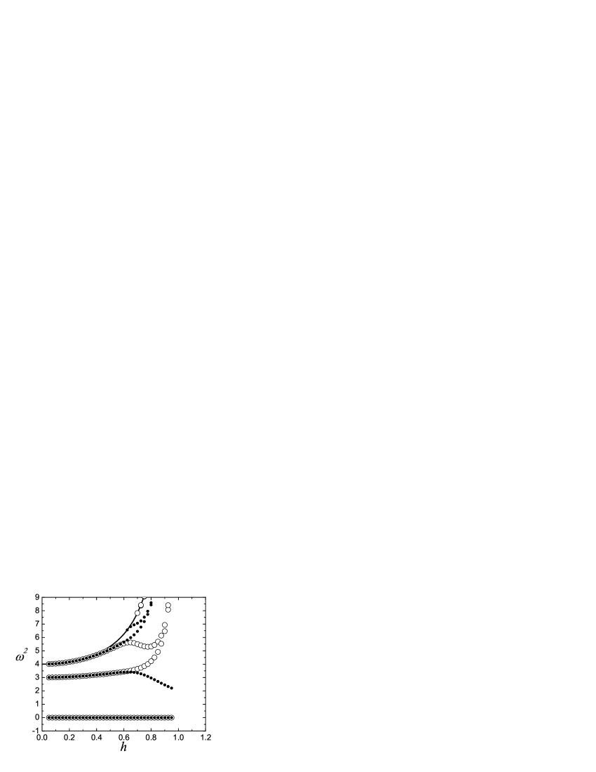
Figure 3: Model 3, Eq. (28): Same as in Fig. 1. The vacuum solution $\phi_{n}=\pm 1$ is unstable for $h>1$. The upper edge of the phonon spectrum lies above the scale of the figure. There are three internal modes. A fourth mode appears for $h>0.6$. Note that there is a zero mode for all values of $h$ indicating the absence of a PN barrier.

II.4 Momentum-conserving model 4

Discretizing Eq. (5) as follows,

$$U_{4}\equiv\frac{1+h^{2}}{h^{2}}(\phi_{n}-\phi_{n-1})^{2}-(1-\phi_{n-1}\phi_{n})^{2}=0,$$ (35)

we come to the model reported in the work of KevrekidisPhysD (motivated by its corresponding, so-called Ablowitz-Ladik sibling discretization for the nonlinear Schrödinger equation AL )

$${\ddot{\phi}_{n}} = \frac{U_{4}(\phi_{n},\phi_{n+1})-U_{4}(\phi_{n-1},\phi_{n})}{\phi_{n+1}-\phi_{n-1}}$$ (36)

$$= \Delta_{2}\phi_{n}+(\phi_{n+1}+\phi_{n-1})(1-\phi_{n}^{2}).$$

This non-Hamiltonian PNb-free model conserves the momentum KevrekidisPhysD which has the form:

$$P_{4}=\sum_{n}\dot{\phi}_{n}(\phi_{n+1}-\phi_{n-1}).$$ (37)

The exact static kink (antikink) solution is

$$\phi_{n}=\pm\tanh[\beta h(n-x_{0})],\quad\tanh(\beta h)=\frac{h}{\sqrt{1+h^{2}}},$$ (38)

where $x_{0}$ is the arbitrary position of the solution.

Alternatively, the kink solution can be found iteratively from

$$\phi_{n}=\frac{\phi_{n-1}\pm h/\sqrt{1+h^{2}}}{1\pm\phi_{n-1}h/\sqrt{1+h^{2}}},$$ (39)

where one can choose either the upper or the lower signs and one can interchange $\phi_{n}$ and $\phi_{n-1}$. To obtain the on-site (inter-site) kink one should use as initial value $\phi_{n}=0$ $(\phi_{n}=\sqrt{1+h^{2}}/h-1/h)$.

The equation of motion, Eq. (36), linearized in the vicinity of an equilibrium solution $\phi_{n}^{0}$ assumes the form

$$\ddot{\varepsilon}_{n}=\left(1+h^{2}\right)\Delta_{2}\varepsilon_{n}+2\varepsilon_{n}-(\phi_{n}^{0})^{2}(\varepsilon_{n-1}+\varepsilon_{n+1})-2\phi_{n}^{0}(\phi_{n-1}^{0}+\phi_{n+1}^{0})\varepsilon_{n}.$$ (40)

The spectrum of vacuum, $\phi_{n}^{0}=\pm 1$, coincides with that of model 1, Eq. (20).

However, the spectrum of the linearization around a kink is different as shown in Fig. 4.

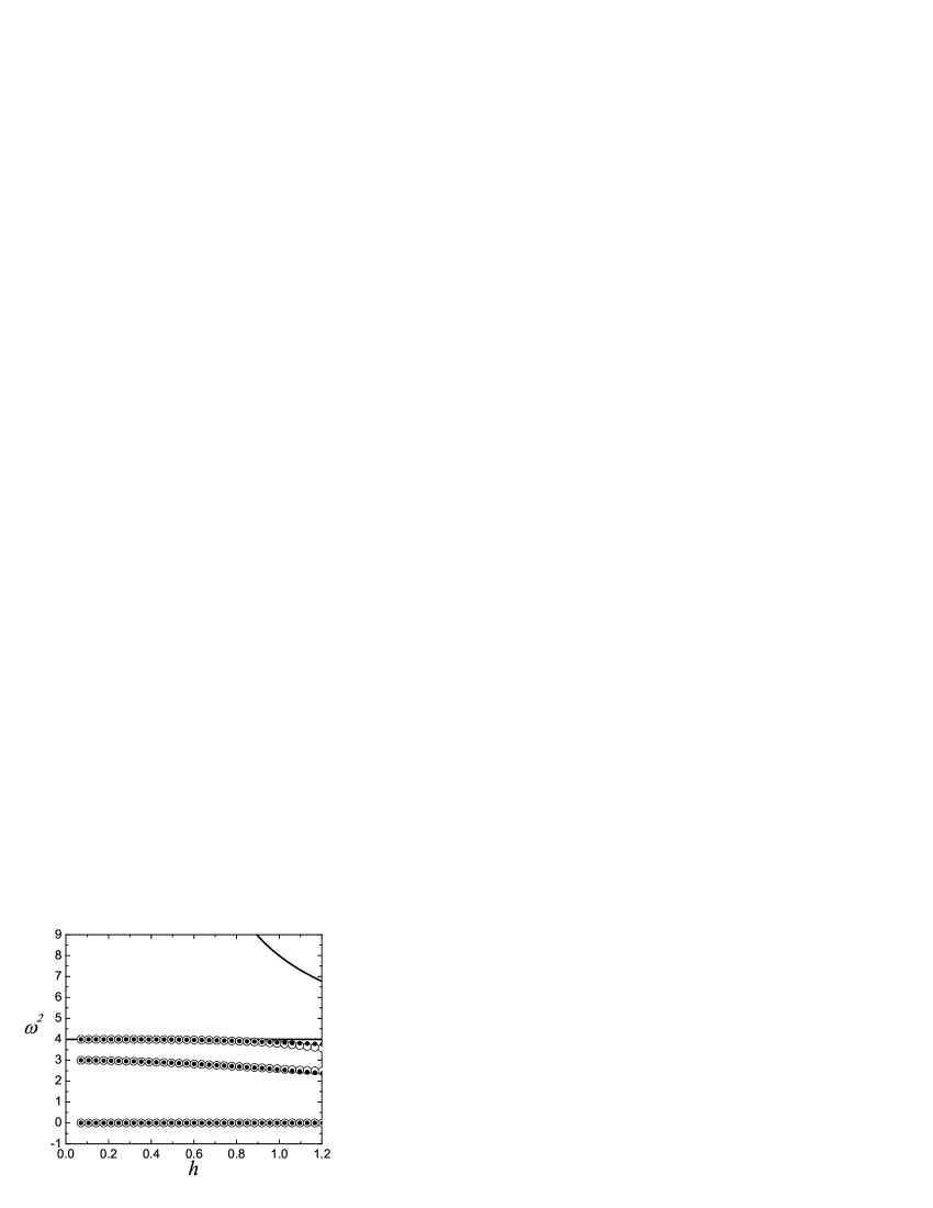
Figure 4: Model 4, Eq. (36). Same as in Fig. 1. There are three internal modes including the $\omega^{2}=0$ mode indicating the absence of a PN barrier.

II.5 Momentum-conserving model 5

Discretizing Eq. (5) as

$$U_{5}\equiv\frac{1}{h^{2}}(\phi_{n}-\phi_{n-1})^{2}-1+\phi_{n-1}^{2}+\phi_{n}^{2}\frac{1}{4}(\phi_{n-1}^{4}+\phi_{n}^{4})-\frac{1}{2}\phi_{n-1}^{2}\phi_{n}^{2}=0,$$ (41)

we obtain another momentum-conserving model of the type of KevrekidisPhysD (see also Barashenkov )

$${\ddot{\phi}_{n}} = \frac{U_{5}(\phi_{n},\phi_{n+1})-U_{5}(\phi_{n-1},\phi_{n})}{\phi_{n+1}-\phi_{n-1}}$$ (42)

$$= \Delta_{2}\phi_{n}+\frac{\phi_{n+1}+\phi_{n-1}}{4}(4-\phi_{n-1}^{2}-2\phi_{n}^{2}-\phi_{n+1}^{2}).$$

This non-Hamiltonian PNb-free model conserves the momentum of Eq. (37).

Static solutions in this model can be found iteratively by solving the quartic Eq. (41).

The equation of motion, Eq. (42), linearized in the vicinity of an equilibrium solution $\phi_{n}^{0}$ is

$$\ddot{\varepsilon}_{n} = \Delta_{2}\varepsilon_{n}+\varepsilon_{n-1}+\varepsilon_{n+1}$$ (43)

$$- \frac{\phi_{n-1}^{0}+\phi_{n+1}^{0}}{2}(\phi_{n-1}^{0}\varepsilon_{n-1}+2\phi_{n}^{0}\varepsilon_{n}+\phi_{n+1}^{0}\varepsilon_{n+1})$$

$$- \frac{\varepsilon_{n-1}+\varepsilon_{n+1}}{4}\left[(\phi_{n-1}^{0})^{2}+2(\phi_{n}^{0})^{2}+(\phi_{n+1}^{0})^{2}\right].$$

The spectrum of vacuum is the same as for model 2, Eq. (26).

Furthermore, the spectrum of the linearization around a kink is shown in Fig. 5.

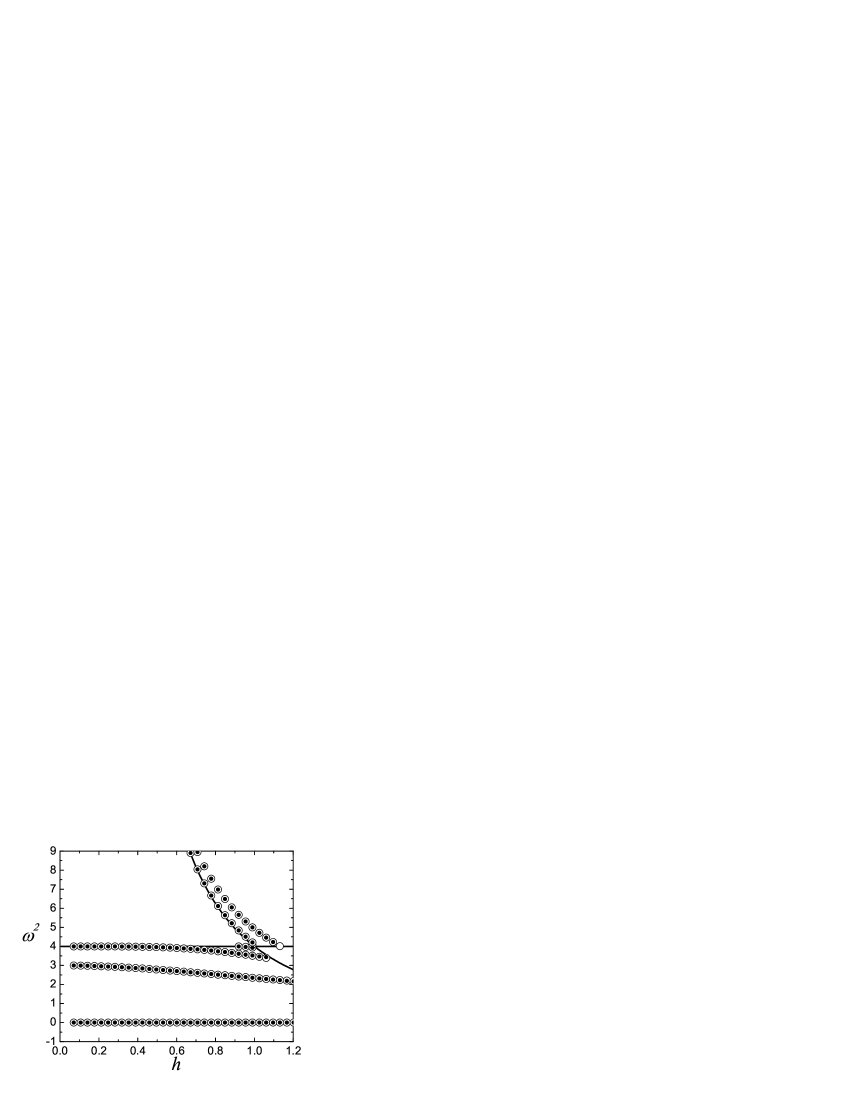
Figure 5: Model 5, Eq. (42). Same as in Fig. 1. A unique feature of this discretization is the presence of the vibrational modes lying above the phonon spectrum. There are three internal modes (including the zero mode) and three additional modes for higher values of $h$ indicating the presence of modes above the phonon spectrum.

III Comparison of Kink Properties

III.1 Spectra of vacuum and kink’s internal modes

We have presented the spectra for the classical $\phi^{4}$ model (model 1) and for the four models free of the Peierls-Nabarro barrier (models 2-5). All models share the same continuum limit; that is why, for small $h$, their properties are close and they only start to deviate from each other, as $h$ increases.

If we divide the models in groups by the quantities they conserve, then models 1-3 belong to the energy-conserving group while models 4 and 5 conserve the momentum of Eq. (37).

Models 3 and 4 have the static solutions derived in Saxena and DKYF . Comparing the DFIs of these models, Eq. (27) and Eq. (35), we can see that the solutions for model 4 can be obtained from those for model 3 by substituting $h\rightarrow h/\sqrt{1+h^{2}}$. Exact static kink solutions are given for model 3 by Eq. (31) or Eq. (32) and for model 4 by Eq. (38) or Eq. (39).

Exact static kink solutions for model 2 can be found iteratively from Eq. (24), while the ones of model 5 can be obtained by solving the quartic Eq. (41). For Model 1, the full 3-point problem of Eq. (10) needs to be solved.

Comparing the spectra of the vacuum (band edges of the spectra are shown by solid lines in Figs. 1 - 5), we note that:

• Model 4 has the same spectrum of vacuum as the classical model 1, and the width of this spectrum vanishes only when $h\rightarrow\infty$. The vacuum solution is always stable because $\omega^{2}>0$ for any $h$.

• Models 2 and 5 have the same spectrum of the vacuum. The width of the spectrum vanishes at $h=1$. Close to this value of $h$, the phonon spectrum is narrow and hence potential phonon radiation (of a kink-like structure due to resonance of internal mode harmonics with the phonon band) is minimized. The vacuum solution is always stable because $\omega^{2}>0$ for any $h$.

• Model 3 has an $h$-dependent cubic term; that is why the lower boundary of the spectrum is also $h$-dependent, while in all other models it is constant ($\omega^{2}=4$). In this model, the vacuum solution is stable only for $0<h<1$.

Subsequently, examining the spectra of lattices containing a static kink, we note that (frequencies of kink’s internal modes are shown in Figs. 1 - 5 by circles and dots):

1. Models 2-5 are PNb-free because they have a zero-frequency mode, which is the, so-called, translational (or the Goldstone) mode of the kink. For model 1, the corresponding mode has a non-zero frequency (in fact, it depends on $h$ as $\propto\exp(-\pi^{2}/h)$; see e.g., pla ), signalling the presence of the Peierls-Nabarro barrier. Given the form of its $h$-dependence, for small $h$ $(<0.4)$, even for model 1 this mode has a nearly zero frequency (see Fig. 1). This is the weakly perturbed translational mode of the continuum $\phi^{4}$ equation.

2. For small $h$ $(<0.4)$ and even for moderate $h$ $(<0.8)$, for all five models, apart from the translational mode we have two kink internal modes lying below the phonon spectrum, one of them very close to the edge of the phonon spectrum ($\omega^{2}=4$) and another one in the vicinity of $\omega^{2}\sim 3$ (i.e., the corresponding continuum limit of this mode sugiyama ). Additional internal modes may emerge for large $h$, but we will focus on smaller values of $h$ (i.e., for $h<0.5$) in the collision results that follow, hence we do not discuss these further here.

3. Model 5, in contrast to all other models, is the model with internal modes lying not only below but also above the phonon band. Such modes, in contrast to the previously reported ones below the band, are of the short-wave (staggered) type and, for this reason, their excitation (or lack thereof) can be sensitive to the position of the collision point with respect to the lattice.

III.2 Static kink profile and kink boosting

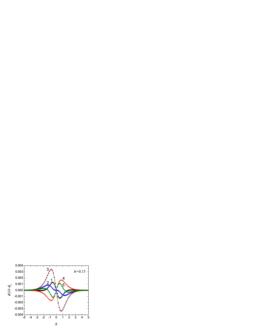
Figure 6: Difference between the continuum and the discrete static kink profiles in the five models at $h=0.15$. The continuum static kink is given by Eq. (4) with $v=0$. The kink in model 3 has the largest deviation from the continuum kink profile. Kinks in the energy-conserving discrete models (1 to 3) have a width smaller than the continuum kink while for the momentum-conserving models 4 and 5, the situation is reversed.

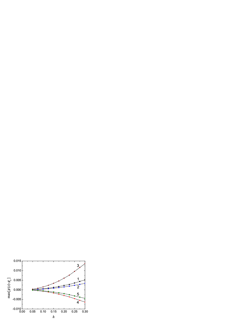
Figure 7: The maximal difference between the continuum and the discrete static kink profiles shown as a function of the spacing $h$ for the five models. The amplitude of the deviation from the continuum kink profile increases with the discreteness parameter as $h^{2}$.

It is also of interest to compare the static kink profiles in the five discrete models (to examine the relevant deviations between them and the continuum limit from which they are derived). In Fig. 6 we present the difference between the static kink profiles of the different models and that of the continuum static kink, Eq. (4). The lattice spacing is $h=0.15$. It is clear that the kink in the CKMS model 3 has the largest deviation from the continuum kink profile. Kinks in the energy-conserving discrete models (1 to 3) have widths which are smaller than that of the continuum kink while for the momentum-conserving models 4 and 5 the situation is reversed. Furthermore, in Fig. 7, we show how this difference between continuum and discrete kink is amplified as $h$ is increased. This is carried out by showing the maximal difference between the two kinks as an $h$-dependent diagnostic which reveals that the relevant difference grows as $h^{2}$ as $h$ increases.

Figure 8: Kinetic energy of a lattice containing a kink boosted at $t=0$ with $v=0.25$ with the help of Eq. (44) for the five discrete models. The lattice spacing is $h=0.3$.

In order to induce collisions, the kink needs to be set into motion in the discrete system. This can be achieved in a variety of ways. Here we have used the most standard one, namely Lorentz boosting the static kink to speed $v$, according to the continuum ansatz:

$$\phi(x,t)=\pm\tanh\frac{h(n-x_{0})-vt}{\sqrt{1-v^{2}}}.$$ (44)

The results presented previously about the static kink also have a direct bearing on the kink boosting. In Fig. 8 we show the kinetic energy of a lattice containing a kink boosted at $t=0$ with velocity $v=0.25$ through Eq. (44). Lines of different thickness show the results for the five discrete models. The lattice spacing is $h=0.3$ in this figure (even though similar, yet less pronounced results have been obtained for smaller $h$; again the relevant trend is quadratic in $h$). $E_{K}(t)$ oscillates with the frequency close to the kink internal mode frequency of $\omega^{2}\sim 3$. At $t=0$ we have $E_{K}=0.043$ and for the energy-conserving models 1 to 3, $E_{K}(t)$ is below this value, while for the momentum-conserving models 4 and 5, it is above this value. This is in sync with the static results where it was shown that models 4 and 5 have a correction to the continuum kink profile of opposite sign than the models 1 to 3 (see also Fig. 6). Model 3 shows the largest amplitude of kinetic energy oscillations, again in agreement with the static results.

We have investigated another boosting method that uses the dynamical solution of the form $\phi_{n}(t)=\phi_{n}^{0}+vt\varepsilon_{n}$, where $\phi_{n}^{0}$ is the static kink solution, $\varepsilon_{n}$ is the normalized translational kink’s internal mode corresponding to the multiple eigenvalue $\omega^{2}=0$, and $v$ is the amplitude that plays the role of kink’s velocity. We found this method to be very good (internal modes were not excited for any $h$) for small $v$, as it should be, because the accuracy of the linearized equations of motion increases as the eigenmode amplitude decreases. However, for velocities of order of $v\sim 0.1$ the accuracy of this method is insufficient because it does not take into account the Lorentz correction of kink’s width. The ansatz Eq. (44) takes into account this correction, but it does not take into account the discreteness of media and, hence, naturally it is less accurate for large $h$.

The best results were obtained for the use of Eq. (44) together with the addition of the kink’s internal mode with the amplitude chosen to compensate the excitation of such mode. In the present study we did not use this more complicated/fine tuned method.

As a result of these considerations, even for relatively small $h$, the kink boosted employing Eq. (44) carries an internal mode of non-vanishing amplitude. This internal mode often plays a nontrivial role in determining the outcome of the collision in what follows.

IV Collision Results

IV.1 Numerical findings for different lattice spacings, initial speeds and kink-antikink separations

We have carried out a comparative study of kink collisions under different discretizations. Our results have been obtained for different domain sizes (i.e., lattice sizes) and with different initial separations detailed in Table 1. As illustrated above, all of our models share the same continuum limit. We have compared the scattering properties for four different (dimensionless) velocities $v=0.21,0.225,0.24$ and $0.255$, respectively presented in Tables 2-5. We chose these velocities motivated by their (continuum limit) phenomenology in the detailed examination of anninos . In each of the Tables 2-5, the collision results are shown with an increment of $0.025$ in the lattice spacing $h$ for each of the different selected initial separations and domain sizes. Some of the standard collision outcomes are highlighted for $v=0.255$ in Figs. 9-13. The most typical cases are those of figures 9-10; the former shows a bion formation (i.e., the kink and the antikink merge, forming an oscillatory, so-called bion state, and never separate thereafter), a behavior typical for sufficiently small speeds. The latter illustrates what is characterized as a “one-bounce” separation, a behavior typical for sufficiently large initial speeds. However, the delicate structure of collisions for an intermediate range of speeds may lead to additional fine structure including multiple bounces before the eventual separation of the two kinks, as illustrated in Figs. 11-13.

Table 1: Domain Sizes and Initial Kink Separations (in units of lattice constant) Examined

domain size	80	80	160
separation	14	28	28

Table 2: Outcome of Kink-Antikink Collisions for $v=0.21$.

Results for velocity 0.21

$h$

Campbell et.al.

Speight

CKMS

K1

K2

80/14

80/28

160/28

80/14

80/28

160/28

80/14

80/28

160/28

80/14

80/28

160/28

80/14

80/28

160/28

0.025

bion

bion

bion

bion

bion

bion

bion

bion

bion

bion

bion

bion

bion

bion

bion

0.05

bion

bion

bion

bion

bion

bion

bion

bion

bion

bion

bion

bion

bion

bion

bion

0.075

bion

bion

bion

bion

bion

bion

bion

bion

bion

bion

bion

bion

bion

bion

bion

0.1

bion

bion

bion

bion

bion

bion

bion

bion

bion

bion

bion

bion

bion

bion

bion

0.125

bion

bion

bion

4

bion

bion

bion

bion

bion

bion

bion

bion

2

2

2

0.15

bion

bion

bion

4

4

bion

bion

bion

bion

bion

bion

bion

4

bion

bion

0.175

bion

bion

bion

bion

bion

3

bion

bion

bion

2

2

2

bion

bion

bion

0.2

bion

bion

bion

bion

bion

2

bion

bion

bion

bion

bion

bion

bion

2

2

0.225

bion

bion

bion

2

bion

bion

bion

3

3

bion

bion

bion

1

1

1

0.25

3

bion

bion

1

1

1

bion

bion

bion

2

2

2

1

1

1

0.275

bion

bion

bion

1

1

1

2

1

1

bion

bion

bion

1

1

1

0.3

2

bion

bion

1

1

1

bion

1

1

bion

2

2

1

1

1

0.325

2

2

2

1

1

1

2

1

1

2

1

1

1

1

1

Table 3: Outcome of Kink-Antikink Collisions for $v=0.225$.

Results for velocity 0.225
$h$	Campbell et.al.			Speight			CKMS			K1			K2
	80/14	80/28	160/28	80/14	80/28	160/28	80/14	80/28	160/28	80/14	80/28	160/28	80/14	80/28	160/28
0.025	2	2	2	2	2	2	2	2	2	2	2	2	2	2	2
0.05	2	2	2	2	2	2	2	2	2	2	2	2	2	2	2
0.075	2	2	2	3	bion	bion	2	2	2	2	2	2	bion	bion	bion
0.1	2	2	2	bion	bion	bion	bion	bion	bion	bion	bion	bion	bion	bion	bion
0.125	2	bion	bion	2	2	2	4	bion	bion	bion	bion	bion	bion	bion	bion
0.15	bion	bion	bion	bion	2	2	bion	bion	bion	bion	bion	bion	bion	2	2
0.175	bion	bion	bion	bion	bion	bion	bion	bion	bion	bion	2	2	bion	bion	bion
0.2	bion	bion	bion	2	bion	1	bion	bion	bion	bion	bion	bion	1	1	1
0.225	3	bion	bion	1	1	1	1	bion	bion	bion	2	2	1	1	1
0.25	2	2	2	1	1	1	1	bion	bion	bion	2	2	1	1	1
0.275	bion	bion	bion	1	1	1	1	1	1	1	1	1	1	1	1
0.3	2	bion	bion	1	1	1	1	1	1	1	1	1	1	1	1
0.325	bion	bion	bion	1	1	1	1	1	1	1	1	1	1	1	1

Table 4: Outcome of Kink-Antikink Collisions for $v=0.24$.

Results for velocity 0.24
$h$	Campbell et.al.			Speight			CKMS			K1			K2
	80/14	80/28	160/28	80/14	80/28	160/28	80/14	80/28	160/28	80/14	80/28	160/28	80/14	80/28	160/28
0.025	bion	bion	bion	bion	bion	bion	bion	bion	bion	bion	bion	bion	bion	bion	bion
0.05	bion	bion	bion	bion	bion	bion	bion	bion	bion	bion	bion	bion	bion	bion	bion
0.075	bion	bion	bion	2	2	2	bion	3	3	2	bion	bion	bion	bion	bion
0.1	bion	bion	bion	3	2	2	bion	2	2	bion	2	2	bion	2	2
0.125	bion	bion	bion	bion	bion	bion	bion	bion	bion	3	3	3	2	bion	bion
0.15	bion	2	2	2	1	1	bion	bion	bion	bion	3	3	1	1	1
0.175	bion	bion	bion	1	1	1	bion	bion	bion	bion	bion	bion	1	1	1
0.2	2	2	2	1	1	1	2	3	3	1	2	2	1	1	1
0.225	2	bion	bion	1	1	1	bion	3	3	1	1	1	1	1	1
0.25	bion	2	2	1	1	1	bion	bion	bion	1	1	1	1	1	1
0.275	bion	2	2	1	1	1	2	1	1	1	1	1	1	1	1
0.3	bion	bion	bion	1	1	1	1	1	1	1	1	1	1	1	1
0.325	2	2	2	1	1	1	1	1	1	1	1	1	1	1	1

Table 5: Outcome of Kink-Antikink Collisions for $v=0.255$.

Results for velocity 0.255
$h$	Campbell et.al.			Speight			CKMS			K1			K2
	80/14	80/28	160/28	80/14	80/28	160/28	80/14	80/28	160/28	80/14	80/28	160/28	80/14	80/28	160/28
0.0125	bion	bion	bion	bion	bion	bion	bion	bion	bion	3	bion	bion	bion	bion	bion
0.025	bion	bion	bion	2	bion	2	bion	bion	bion	bion	bion	bion	2	2	2
0.05	2	bion	bion	bion	2	2	bion	bion	bion	2	2	2	2	4	4
0.075	bion	bion	bion	1	bion	2	bion	2	2	bion	2	1	1	1	1
0.1	2	bion	bion	1	1	1	1	bion	bion	1	1	1	1	1	1
0.125	bion	bion	bion	1	1	1	1	bion	bion	1	1	1	1	1	1
0.15	1	3	3	1	1	1	1	2	2	1	1	1	1	1	1
0.175	1	bion	4	1	1	1	1	2	2	1	1	1	1	1	1
0.2	1	1	1	1	1	1	1	1	1	1	1	1	1	1	1
0.225	1	1	1	1	1	1	1	1	1	1	1	1	1	1	1
0.25	1	1	1	1	1	1	1	1	1	1	1	1	1	1	1
0.275	1	1	1	1	1	1	1	1	1	1	1	1	1	1	1
0.3	1	1	1	1	1	1	1	1	1	1	1	1	1	1	1
0.325	1	1	1	1	1	1	1	1	1	1	1	1	1	1	1

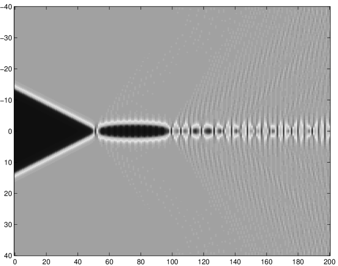
Figure 9: Bion formation for model 3 with h = 0.05, kink velocity = 0.255, domain size = 80, kink separation = 28. Note the radiation (phonons) emanating from the bion.

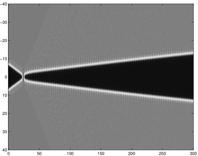
Figure 10: One bounce for model 2 with h = 0.1, kink velocity = 0.255, domain size = 80, kink separation = 14.

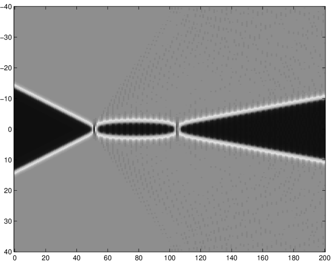
Figure 11: Two bounces for model 4 with h = 0.05, kink velocity = 0.255, domain size = 80, kink separation = 28.

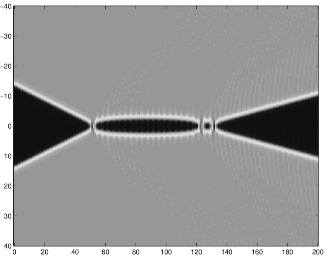
Figure 12: Three bounces for model 1 with h = 0.15, kink velocity = 0.255, domain size = 80, kink separation = 28.

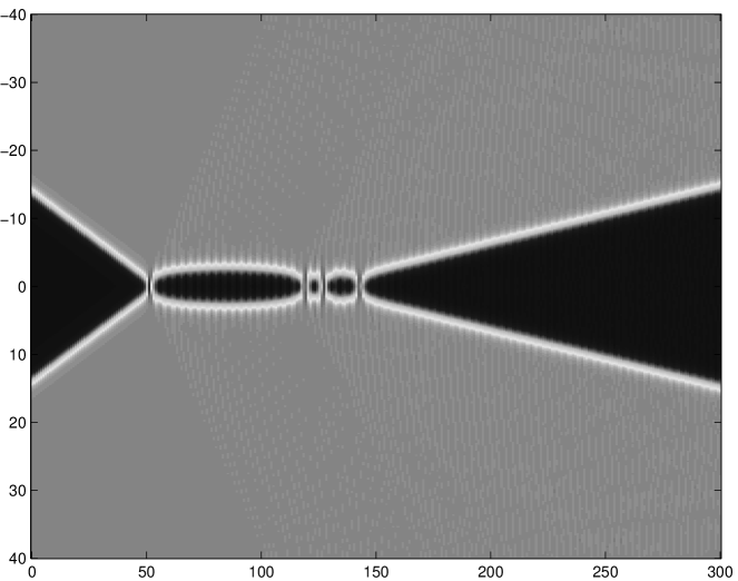
Figure 13: Four bounces for model 5 with h = 0.05, kink velocity = 0.255, domain size = 80, kink separation = 28.

The general trend as displayed in the table 2 is that for velocity $v=0.21$, when the kinks collide, they form a bion state. In the bound state the kink and the antikink are trapped by their mutual attraction. In the table we see that, for small lattice spacings, the behavior of the different models is similar (as is expected, given the common continuum limit); on the other hand, the dynamics starts to diversify between discretizations, as the spacing is increased. Remarkably so, for larger values of $h$, we observe that the collisions are more elastic and, in fact, typically result in a single bounce for sufficiently large $h$. For velocity $v=0.225$ (Table 3) the kinks are in a two-bounce window for small lattice spacing $h$ but the change in outcome with increasing $h$ is rather drastic (especially since the two-bounce is a rather fine-tuned collision outcome, where the internal modes control the resonant transfer of energy from and back to its original kinetic form anninos ; Campbell ; goodman ). We see a similar trend for the case with velocity $v=0.24$, whereby the kinks form a bion state in the continuum limit but for increasing $h$ we observe multiple bounces. For higher $h$, the kinks in all five models collide quasi-elastically i.e., with a single bounce. For a kink velocity of $v=0.255$ (which is close to the critical velocity, above which only single bounce phenomena occur in the continuum) we see an additional quite interesting feature. In this case, the outcomes for different models are so sensitive that they may not even converge for very small values of $h$.

Our results overall indicate that the elasticity of the collisions depends strongly on the lattice spacing as well as on the details of the particular discretization. The collisions appear to be more elastic for larger values of $h$, a feature which seems to be counter-intuitive given that discreteness in this type of models is perceived as a source of dissipation of kinetic energy peyrard1 . On the other hand, discreteness leads to the excitation of additional internal modes (see Figs. 2, 3 and 5, in particular) and hence, potentially, to more exotic dynamical outcomes of the collisions. Furthermore, as $h$ increases the width of the phonon band decreases, hence potentially limiting the range of resonant modes and therefore the amount of radiated energy (see also the relevant discussion below). This particular feature (apparent collision elasticity increase as a function of $h$) would be certainly wortwhile of a separate and detailed theoretical investigation. From the general trends of our results, we also observe that the most inelastic collisions occur for model 1, as might be expected by the presence of the PN barrier in that model. Finally, one more note of caution worth making here concerns the disparity between the different model results even for small $h$. It is clear that such phenomena as the outcome of collisions depend strongly and sensitively on a variety of factors (including e.g., the internal mode excitations, the location of collision, etc.) to an extent that one should not expect identical collision outcomes among these models even rather close to the continuum limit (which the models share). This is also a result that partially defies the conventional wisdom that would suggest that different collisional outcomes across discretizations might be expected only when the length scale of discreteness (the lattice spacing) becomes comparable to the size of the kink.

In what follows, we briefly analyze one of the sources of the above mentioned sensitivity of the collision outcome, namely the original distance between the kink-antikink pair. We also quantify in a characteristic, in our view, way the increase in collision elasticity through the dependence of the critical speed separating bion formation from one-bounce collisions as a function of the lattice spacing $h$.

IV.2 Initial distance between colliding kinks

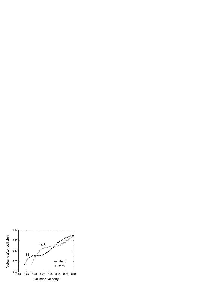
Figure 14: Kink velocity after collision as a function of collision velocity in model 3 at $h=0.15$. Dots show the results for initial distance between kinks of $14$, while open circles for the initial distance of $14.8$.

In Fig. 14 we show the kink velocity after the collision as a function of initial collision velocity in model 3 at $h=0.15$. Dots show the results for initial distance between kinks of $14$, while open circles for the initial distance of $14.8$.

One can notice a strong sensitivity of the collision outcome to the initial separation distance. This is because of the internal mode being excited when boosting the kinks. Changing the initial distance, we change the phase of the internal mode at the collision point, which critically, in turn, affects the result of the collision.

For different models, the sensitivity of the collision outcome to the initial kink separation correlates with the amplitude of the kink’s internal mode excited at boosting (see Fig. 8). Thus, the sensitivity is highest for model 3 and lowest for model 5.

The sensitivity also decreases rapidly with decrease in $h$ and the reason is, essentially, the same: the amplitude of the excited kink’s internal mode decreases as $h^{2}$.

IV.3 Threshold velocity $v_{c}$ as a function of $h$

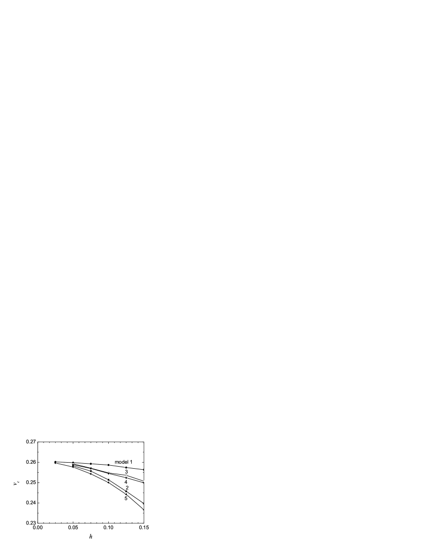
Figure 15: Critical velocity $v_{c}$ as a function of $h$ for the five models. In all models, $v_{c}$ decreases with increase in $h$ implying that for larger $h$ collisions are more elastic. The classical discretization (model 1) shows the weakest dependence of $v_{c}$ on $h$, while in the models 2 and 5 this dependence is strongest.

It is well known (see, e.g., Campbell ) that there exists a threshold velocity $v_{c}$ such that collision of kinks with $v>v_{c}$ leads to separation after the first collision while for collisions with $v<v_{c}$, the first collision cannot lead to separation. In the latter case, the reflection windows discussed in Campbell can be observed amidst regions of bion formation.

In Fig. 15 we show for the five models how $v_{c}$ changes with $h$. These results were obtained from computations similar to the ones presented in Fig. 14; $v_{c}$ was estimated from the fit ${\rm constant}\times(v^{2}-v^{2}_{c})^{1/2}$ suggested in Campbell and thus the effect of the initial separation was averaged out to some extent.

In all models $v_{c}$ decreases with increase in $h$ implying that for larger $h$ the collisions are more elastic. The standard discretization (model 1) shows the weakest dependence of $v_{c}$ on $h$, while in models 2 and 5 this dependence is strongest.

Since the PN barrier is very small at $h\sim 0.1$, the observed effect can hardly be explained through the influence of the PN barrier. As one possible explanation of the dependence of $v_{c}$ on $h$, we discuss the burst of radiation emitted during collision. Corresponding numerical results are presented in Fig. 16 for kinks colliding with $v=0.26$ in the Speight lattice (model 2) with two lattice spacings, $h=0.1$ and $h=0.15$. This is the highest velocity we use in our simulations. We show the kinetic energy of radiation, (in order to exclude the kinetic energy of the moving kinks, an area of width equal to 4 around each kink was not included in the computation of the kinetic energy) as a function of the time after collision. Dots show the results for $h=0.1$ and open circles for $h=0.15$. The amount of radiated energy grows with time due to the emission from the kink’s internal modes excited at the collision.

Extrapolation of the data presented in Fig. 16 to $t=0$ suggests that, in the case of $h=0.1$, the collision results in the burst of kinetic energy (in dimensionless units) of $8.7\times 10^{-3}$, while a smaller burst of radiation of $6.8\times 10^{-3}$ takes place in the lattice with higher discreteness of $h=0.15$. The fact that the burst of radiation is smaller in the lattice with higher discreteness can be related to the phonon spectrum width, which decreases with $h$ as $1/h$ for small $h$, for all five models. The narrower the phonon band, the smaller the amount of energy that can be radiated and the more elastic the collision.

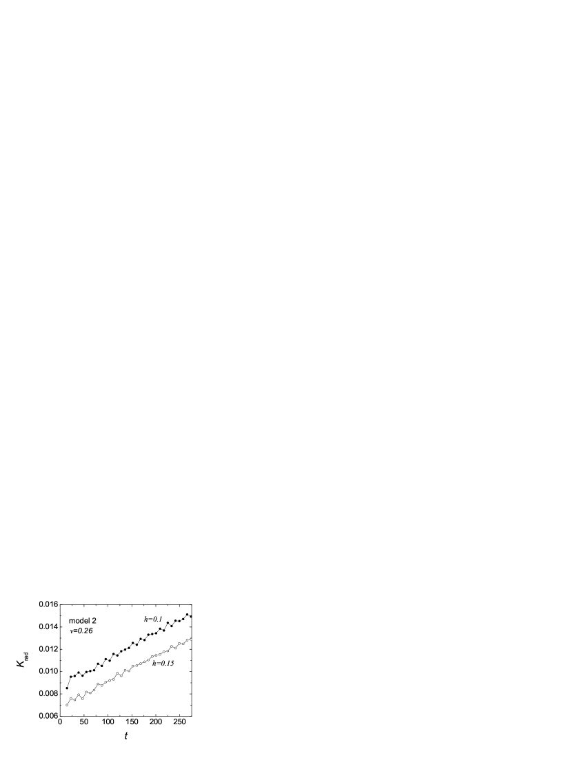
Figure 16: Kinetic energy of radiation as a function of the time after a collision in model 2. Dots show the results for the lattice spacing $h=0.1$ and open circles for $h=0.15$. The collision velocity is $v=0.26$. Radiated energy growth with time is due to the coupling of the kink’s internal modes with the phonon band. Extrapolation of the data to $t=0$ suggests that in the case of $h=0.1$ collision results in the burst of (dimensionless) kinetic energy of $8.7\times 10^{-3}$, while a smaller burst of radiation of $6.8\times 10^{-3}$ takes place in a lattice with higher discreteness of $h=0.15$.

V Conclusions and Future Challenges

In the present work, we have analyzed the properties of a number of recently proposed discretizations of the continuum $\phi^{4}$ field theory in the vicinity of (and further away from) the continuum limit. The relevant analysis consisted of the examination of the static properties of the models, concerning their fundamental nonlinear wave solutions, namely the kinks (and anti-kinks). For these types of solutions, we have examined how to obtain them, in what ways they differ from their continuum siblings, as well as the spectral properties of the linearization around such solutions. In particular, we have computed both the phonon (continuous) spectrum, as well as discussed the internal (or shape) modes present in the models.

On the other hand, we have also examined dynamic properties of the kinks by studying their collision and comparing/contrasting their outcomes across the different discretizations. In that regard, we have observed a variety of interesting results. In particular, we have seen that the models only align with their continuum limit (especially as regards sensitive collision phenomenology) extremely close to the continuum limit [(i.e., for spacings of O$(10^{-2})$)]. In fact, in some cases (e.g. for the CKMS model and $v=0.255$), the results are not independent of factors such as lattice spacing and kink-antikink separation even for the smallest $h$ used herein ($h=0.0125$). This is rather remarkable given that the scale of the kinks themselves is considerably wider, hence one would not expect this result on the basis of length-scale competition. However, we have argued that this should be attributed to the (initial-boost induced) excitation of the internal modes of the kink whose coupling to the continuous spectrum sensitively affects the collision outcome, as has been substantiated previously anninos ; Campbell ; Campbell1 ; goodman . This should operate as a significant note of caution to researchers conducting numerical experiments with these models in an attempt to describe their continuum limits.

Furthermore, we have seen that the elasticity of collisions varies not only from model to model, but even with increasing spacing of the lattice. In particular, we have illustrated through our numerical observations that the most inelastic collisions take place in the model that does have a Peierls-Nabarro barrier, while PNb-free models feature more elastic collisions. Moreover, there is a very interesting (and worthwhile to investigate further, possibly theoretically as well) dependence of the critical speed for single-bounce collisions on the spacing $h$. In particular, $v_{c}$ rapidly decreases as a function of $h$, rendering coarser collisions more elastic. This should also be attributed to the spectral properties of the models and the decreasing width of the phonon band for increasing $h$, which activates fewer couplings of internal mode frequency harmonics with the continuous spectrum and hence leads to weaker “dissipation” and consequently to more elastic collisions.

While the static properties of the kinks have been obtained to a large extent explicitly from the underlying discretized first integral formalisms, kink collisions are naturally much harder to analyze theoretically for the presented discrete models. However, some of the relevant features such as the dependence of $v_{c}$ on $h$ may be, to a certain degree, tractable (see e.g. goodman and references therein). Hence, it would be particularly interesting to seek a deeper understanding of the features numerically observed herein and how these can be associated with the nature of the underlying discretized nonlinearity. Such studies are currently in progress.

References

- (1) V. V. Konotop and V. A. Brazhnyi, Mod. Phys. Lett. B 18 627, (2004); P.G. Kevrekidis and D. J. Frantzeskakis, Mod. Phys. Lett. B 18, 173 (2004).
- (2) D. N. Christodoulides, F. Lederer, and Y. Silberberg, Nature 424, 817 (2003); Yu. S. Kivshar and G. P. Agrawal, Optical Solitons: From Fibers to Photonic Crystals, Academic Press (San Diego, 2003).
- (3) M. Peyrard, Nonlinearity 17, R1 (2004).
- (4) O. M. Braun and Y. S. Kivshar, The Frenkel-Kontorova Model: Concepts, Methods, and Applications (Springer, Berlin, 2004).
- (5) T. I. Belova and A. E. Kudryavtsev, Phys. Usp. 40, 359 (1997).
- (6) P. Anninos, S. Oliveira, and R.A. Matzner, Phys. Rev. D 44, 1147 (1991).
- (7) D. K. Campbell, J. F. Schonfeld, and C. A. Wingate, Physica D 9, 1 (1983).
- (8) D.K. Campbell and M. Peyrard, Physica D 18, 47 (1986); ibid. 19, 165 (1986).
- (9) R.H. Goodman and R. Haberman, SIAM J. Appl. Dyn. Sys. 4, 1195 (2005).
- (10) C. Sulem and P.L. Sulem, The Nonlinear Schrödinger Equation, (Springer-Verlag, New York, 1999).
- (11) J. M. Speight, Nonlinearity 12, 1373 (1999).
- (12) J. M. Speight and R. S. Ward, Nonlinearity 7, 475 (1994).
- (13) J. M. Speight, Nonlinearity 10, 1615 (1997).
- (14) E. B. Bogomol’nyi, J. Nucl. Phys. 24, 449 (1976).
- (15) P. G. Kevrekidis, Physica D 183, 68 (2003).
- (16) F. Cooper, A. Khare, B. Mihaila, and A. Saxena, Phys. Rev. E 72, 36605 (2005).
- (17) S. V. Dmitriev, P. G. Kevrekidis, and N. Yoshikawa, J. Phys. A 38, 7617 (2005).
- (18) I. V. Barashenkov, O. F. Oxtoby, and D. E. Pelinovsky, Phys. Rev. E 72, 035602(R) (2005); O. F. Oxtoby, D. E. Pelinovsky, and I. V. Barashenkov, Nonlinearity 19, 217 (2006).
- (19) S.V. Dmitriev, P.G. Kevrekidis, A.A. Sukhorukov, N. Yoshikawa, and S. Takeno, Phys. Lett. A 356, 324 (2006); P. G. Kevrekidis, S. V. Dmitriev, and A. A. Sukhorukov, nlin.SI/0603046.
- (20) D.E. Pelinovsky, nlin.PS/0603022.
- (21) A. Khare, K. Ø. Rasmussen, M. R. Samuelsen, and A. Saxena, J. Phys. A: Math. Gen. 38, 807 (2005); A. Khare, K. Ø. Rasmussen, M. Salerno, M. R. Samuelsen, and A. Saxena, Phys. Rev. E 74, 016607 (2006).
- (22) A.B. Adib and C.A.S. Almeida, Phys. Rev. E 64, 037701 (2001).
- (23) M. J. Ablowitz and J. F. Ladik, J. Math. Phys. 16, 598 (1975); M. J. Ablowitz and J. F. Ladik, J. Math. Phys. 17, 1011 (1976).
- (24) S. V. Dmitriev, P. G. Kevrekidis, N. Yoshikawa, and D. J. Frantzeskakis, nlin.PS/0603074.
- (25) P. G. Kevrekidis, C.K.R.T. Jones, and T. Kapitula, Phys. Lett. A 269, 120 (2000).
- (26) T. Sugiyama, Prog. Theor. Phys. 61, 1550 (1978).
- (27) M. Peyrard and M.D. Kruskal, Physica D 14, 88 (1984).