Control of the chaotic velocity dispersion of a cold electron beam interacting with electrostatic waves

Abstract

In this article we present an application of a method of control of Hamiltonian systems to the chaotic velocity diffusion of a cold electron beam interacting with electrostatic waves. We numerically show the efficiency and robustness of the additional small control term in restoring kinetic coherence of the injected electron beam.

1 Introduction

The consequences of chaotic dynamics can be harmful in several contexts. During the last decade or so, much attention has been paid to the problem of chaos control. Controlling chaos means that one aims at reducing or suppressing chaos by mean of a small perturbation so that the original structure of the system under investigation is kept practically unaltered, while its behavior can be substantially altered. In particular, in many physical devices there are undesirable effects due to transport phenomena that can be attributed to a chaotic dynamics. For example, chaos in beams of particle accelerators leads to a weakening of the beam luminosity acceleratori ; robin . Similar problems are encountered in free electron lasers boni90 ; deni04 . In magnetically confined fusion plasmas, the so called anomalous transport, which has its microscopic origin in a chaotic transport of charged particles, represents a challenge to the attainment of high performance in fusion devices carre97 . The theoretical description of the physics of these devices (beam accelerators, free electron lasers, fusion devices) is based on Hamiltonian models, thus the above mentioned possibility of harmful consequences of chaos is related with Hamiltonian chaos. One way to control transport would be that of reducing or suppressing chaos. There exist numerous attempts to cope with this problem rev_c_d . However, these efforts have mainly been focused on dissipative systems. For Hamiltonian systems, the absence of phase space attractors has been a hindrance to the development of efficient methods of control. Conventional approaches aim at targeting individual trajectories. However, when a microscopic description of a physical system is required, targeting of individual microscopic trajectories is hopeless.

The strategy we developed is based on a small but suitable modification of the original Hamiltonian system such that the controlled one has a more regular dynamics. In this article this strategy is illustrated through a particular example: how to restore kinetic coherence of a cold electron beam interacting with electrostatic waves. Here chaos deteriorates the velocity ”monochromaticity” of the injected beam and one has to find a strategy of control such that this effect is reduced or suppressed.

The Hamiltonian which models the dynamics of charged test particles moving in electrostatic waves is

$$H(p,x,t)=\frac{p^{2}}{2}+\sum_{n=1}^{N}\varepsilon_{n}\cos(k_{n}x-\omega_{n}t+\varphi_{n}),$$ (1)

where $p$ is the test charged particle momentum and $\varepsilon_{n}$, $k_{n}$, $\omega_{n}$ and $\varphi_{n}$ are respectively the amplitudes, wave numbers, frequencies and phases of the electrostatic waves. Generically, for $N\geq 2$, the dynamics of the particles governed by this equation is a mixture of regular and chaotic behaviours mainly depending on the amplitude of the waves.

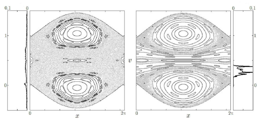
Figure 1: Poincaré surface of section and (normalized) probability distribution functions $F(p)$ of the velocity for the Hamiltonian given by Eq. (1) without control term (left panel) and with the control term given by Eq. (12) (right panel). The depicted numerical results are obtained in the case of two electrostatic waves using $(\varepsilon_{1},k_{1},\omega_{1},\varphi_{1})=(0.045,1,0,0)$ and $(\varepsilon_{2},k_{2},\omega_{2},\varphi_{2})=(0.045,1,1,0)$. Reprinted from Ref. TWT05 .

A Poincaré section of the dynamics (a stroboscopic plot of selected trajectories) is depicted on Fig. 1 for two waves ($N=2$). A large zone of chaotic behaviour occurs in between the primary resonances (nested regular structures). If one considers a beam of initially monokinetic particles, this zone is associated with a large spread of the velocities after some time (left hand side panel of Fig. 1) since the particles are moving in the chaotic sea created by the overlap of the two resonances chir79 . Here the problem of control is to find a control term $f$ given by

$$f(x,t)=\sum_{n=1}^{q}\eta_{n}\cos(\kappa_{n}x-\Omega_{n}t+\Phi_{n}),$$ (2)

that is the right set of additional controlling waves, such that the controlled Hamiltonian

$$H_{c}(p,x,t)=H(p,x,t)+f(x,t),$$

given by the original one plus the control term, is more regular than $H$. In general, adding a generic perturbation adds more resonances and hence more chaos. Nevertheless this problem has some obvious solutions with additional waves having amplitudes of the same order as the initial ones. For energetic purposes, the additional waves must have amplitudes which are much smaller than the initial ones ($\max_{n}|\eta_{n}|\ll\max_{n}|\varepsilon_{n}|$). This means finding a specifically designed small control term that is a slight modification of the system but which drastically changes the dynamical behaviour from chaotic to regular. In particular one aims at building barriers to transport that prevent large scale chaos to occur in the system.

2 Local control method and control term

In this section we briefly sketch the local control method that was extensively discussed in Refs. vitt05 ; chan05 . Let us consider Hamiltonian systems of the form

$$H({\bf A},{\bm{\theta}})=H_{0}({\bf A})+\varepsilon V({\bf A},{\bm{\theta}}),$$

that after a suitable expansion can be rewritten as

$$H({\bf A},{\bm{\theta}})={\bm{\omega}}\cdot{\bf A}+\varepsilon v({\bm{\theta}})+w({\bf A},{\bm{\theta}}),$$ (3)

where $({\bf A},{\bm{\theta}})\in{\mathbb{R}}^{L}\times{\mathbb{T}}^{L}$ are action-angle variables for $H_{0}$ in a phase space of dimension $2L$. The last term of the expansion can be written as

$$w({\bf A},{\bm{\theta}})=\varepsilon{\bf w}_{1}({\bm{\theta}})\cdot{\bf A}+w_{2}({\bf A},{\bm{\theta}}),$$

where $w_{2}$ is quadratic in the actions, i.e. $w_{2}({\bf 0},{\bm{\theta}})=0$ and $\partial_{\bf A}w_{2}({\bf 0},{\bm{\theta}})={\bf 0}$. We assume that $\bm{\omega}$ is a non-resonant vector of ${\mathbb{R}}^{L}$, i.e. there is no non-zero ${\bf k}\in{\mathbb{Z}}^{L}$ such that ${\bm{\omega}}\cdot{\bf k}=0$. Moreover we assume without restrictions that $\int_{{\mathbb{T}}^{L}}v({\bm{\theta}})d^{L}{\bm{\theta}}=0$.

We consider a region near ${\bf A}={\bf 0}$. The controlled Hamiltonian we construct is given by

$$H_{c}({\bf A},{\bm{\theta}})={\bm{\omega}}\cdot{\bf A}+\varepsilon v({\bm{\theta}})+w({\bf A},{\bm{\theta}})+\varepsilon^{2}f({\bm{\theta}}).$$ (4)

The control term depends only on angle variables and its expression is given by

$$f({\bm{\theta}})=-\varepsilon^{-2}w(-\varepsilon\Gamma\partial_{\bm{\theta}}v,{\bm{\theta}}),$$ (5)

where $\partial_{\bm{\theta}}v$ denotes the first derivatives of $v$ with respect to ${\bm{\theta}}$ : $\partial_{\bm{\theta}}v=\sum_{{\bf k}\in{\mathbb{Z}}^{L}}i{\bf k}v_{\bf k}{\mathrm{e}}^{i{\bf k}\cdot{\bm{\theta}}}$ and where the linear operator $\Gamma$ is a pseudo-inverse of ${\bm{\omega}}\cdot\partial_{\bm{\theta}}$, i.e. its action on a function $v({\bm{\theta}})=\sum_{{\bf k}\in{\mathbb{Z}}^{L}}v_{\bf k}{\mathrm{e}}^{i{\bf k}\cdot{\bm{\theta}}}$ is :

$$\Gamma v({\bm{\theta}})=\sum_{{\bf k}\in{\mathbb{Z}}^{L}\setminus\{{\bf 0}\}}\frac{v_{\bf k}}{i{\bm{\omega}}\cdot{\bf k}}{\mathrm{e}}^{i{\bf k}\cdot{\bm{\theta}}}.$$ (6)

We prove (see Ref. chan05 ) that $H_{c}$ has an invariant torus located at ${\bf A}=-\varepsilon\Gamma\partial_{\bm{\theta}}v$. For Hamiltonian systems with two degrees of freedom, such an invariant torus acts as a barrier to diffusion. For the construction of the control term, we notice that we do not require that the quadratic part of $w$ is small in order to have a control term of order $\varepsilon^{2}$.

2.1 Control term for a two wave model

We consider the following Hamiltonian with two traveling waves:

$$H(p,x,t) = \frac{p^{2}}{2}+\varepsilon_{1}\cos(k_{1}x-\omega_{1}t+\varphi_{1})$$ (7)

$$+\varepsilon_{2}\cos(k_{2}x-\omega_{2}t+\varphi_{2}),$$

where the wavenumbers are chosen according to a given dispersion relation $k_{1}=K(\omega_{1})$ and $k_{2}=K(\omega_{2})$. The numerical results we will show in the following have been obtained using $(\varepsilon_{1},k_{1},\omega_{1},\varphi_{1})=(\varepsilon,1,0,0)$ and $(\varepsilon_{2},k_{2},\omega_{2},\varphi_{2})=(\varepsilon,1,1,0)$. Similar results are expected for other values of $(\varepsilon_{n},k_{n},\omega_{n},\varphi_{n})$.

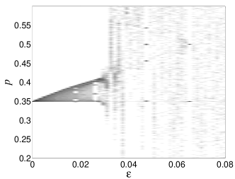
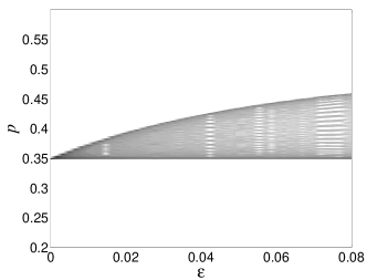
Figure 2: Distribution of momenta $p$ as a function of $\varepsilon$ for Hamiltonian (7) (left panel) and for Hamiltonian (7) plus the control term (10) (right panel). The numerical results are obtained for the following values of the parameters: $(\varepsilon_{1},k_{1},\omega_{1},\varphi_{1})=(\varepsilon,1,0,0)$ and $(\varepsilon_{2},k_{2},\omega_{2},\varphi_{2})=(\varepsilon,1,1,0)$.

Figure 2 (left panel) depicts the probability distribution function of the momenta of a trajectory of Hamiltonian (7) for $t\in[0,800\pi]$ (with initial condition chosen in the chaotic sea, e.g. for $(p\approx 0.35,x=0)$) as a function of the amplitude $\varepsilon$ of the perturbation. It shows that after $\varepsilon_{c}\approx 0.028$ there is no longer any barrier in phase space. We notice that the value of $\varepsilon_{c}$ for which the last invariant torus is broken is approximately equal to $\varepsilon_{c}\approx 0.02759$ chan02 .

The first step in order to compute the local control term which recreates a barrier in phase space is to map this Hamiltonian with one and a half degrees of freedom into an autonomous Hamiltonian with two degrees of freedom by considering that $t\mbox{ mod }2\pi$ is an additional angle variable. We denote $E$ its conjugate action. The autonomous Hamiltonian is

$$H = E+\frac{p^{2}}{2}+\varepsilon_{1}\cos(k_{1}x-\omega_{1}t+\varphi_{1})$$ (8)

$$+\varepsilon_{2}\cos(k_{2}x-\omega_{2}t+\varphi_{2}).$$

Then, the momentum $p$ is shifted by $\omega$ in order to define a local control in the region $p\approx 0$. The Hamiltonian is rewritten as

$$H = E+\omega p+\varepsilon_{1}\cos(k_{1}x-\omega_{1}t+\varphi_{1})$$ (9)

$$+\varepsilon_{2}\cos(k_{2}x-\omega_{2}t+\varphi_{2})+\frac{p^{2}}{2}.$$

We define

$$H_{0}=E+\omega p,$$

$$v(x,t)=\varepsilon_{1}\cos(k_{1}x-\omega_{1}t+\varphi_{1})+\varepsilon_{2}\cos(k_{2}x-\omega_{2}t+\varphi_{2}),$$

$$w(p,x,t)=p^{2}/2,$$

provided $\omega\neq\omega_{1}/k_{1}$ and $\omega\neq\omega_{2}/k_{2}$. In this case the control term is given by

$$f(x,t)=-\frac{1}{2}(\Gamma\partial_{x}v)^{2},$$

where $\partial_{x}$ is the partial derivative with respect to $x$ and the action of $\Gamma$ follows from Eq. (6). Therefore the control term is equal to

$$f(x,t) = -\frac{1}{2}\left[\varepsilon_{1}k_{1}\frac{\cos(k_{1}x-\omega_{1}t+\varphi_{1})}{\omega k_{1}-\omega_{1}}\right.$$ (10)

$$+\left.\varepsilon_{2}k_{2}\frac{\cos(k_{2}x-\omega_{2}t+\varphi_{2})}{\omega k_{2}-\omega_{2}}\right]^{2}.$$

Adding the exact control term (10) to the Hamiltonian (9), an invariant KAM torus with frequency $\omega$ is recreated. This barrier prevents the electron beam to diffuse in phase space and the electron kinetic coherence is restored. In Fig. 2 (right panel) the recreation of barrier in phase space can be observed on the probability distribution function of the momenta of a trajectory of Hamiltonian (7) plus the control term (10) for $t\in[0,800\pi]$ (with initial condition chosen as in the uncontrolled case, e.g. for $(p\approx 0.35,x=0)$). In fact for all the values of the amplitude $\varepsilon$ of the perturbation, the kinetic coherence of the initial electron beam is preserved.

The local control ensures that the barrier persists for all the magnitudes of the perturbation and also gives us explicitly the equation of the recreated KAM torus, that is

$$p_{0}(x,t) = \omega-\varepsilon_{1}k_{1}\frac{\cos(k_{1}x-\omega_{1}t+\varphi_{1})}{\omega k_{1}-\omega_{1}}$$ (11)

$$-\varepsilon_{2}k_{2}\frac{\cos(k_{2}x-\omega_{2}t+\varphi_{2})}{\omega k_{2}-\omega_{2}}.$$

The control term (10) has four Fourier modes, $(2k_{1},-2\omega_{1})$, $(2k_{2},-2\omega_{2})$, $((k_{1}+k_{2}),-(\omega_{1}+\omega_{2}))$ and $((k_{1}-k_{2}),-(\omega_{1}-\omega_{2}))$. If we consider $\omega$ close to $(\omega_{1}/k_{1}+\omega_{2}/k_{2})/2$, the main Fourier mode of the control term is

$$f_{2} = -\frac{\varepsilon_{1}\varepsilon_{2}k_{1}k_{2}}{2(\omega k_{1}-\omega_{1})(\omega k_{2}-\omega_{2})}\times$$ (12)

$$\cos[(k_{1}+k_{2})x-(\omega_{1}+\omega_{2})t+\varphi_{1}+\varphi_{2}].~{}~{}$$

Assuming $\omega=(\omega_{1}/k_{1}+\omega_{2}/k_{2})/2$, the control term given by Eq. (12) is

$$f_{2}=\frac{2\varepsilon_{1}\varepsilon_{2}}{(v_{1}-v_{2})^{2}}\cos[(k_{1}+k_{2})x-(\omega_{1}+\omega_{2})t+\varphi_{1}+\varphi_{2}],$$

where $v_{n}$ is the group velocity of the wave $n$ defined as $v_{n}=\omega_{n}/k_{n}$.

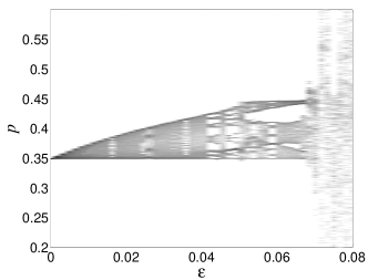
Figure 3: Distribution of momentum $p$ as a function of $\varepsilon$ for Hamiltonian (7) with the approximate control term (12). The numerical results are obtained for the same values of the parameters as in Fig. 2.

Figure 3 depicts the probability distribution function of the momenta of a trajectory of Hamiltonian (7) with the approximate control term (12), for $t\in[0,800\pi]$ and with initial condition $(p\approx 0.35,x=0)$, as a function of the amplitude $\varepsilon$ of the perturbation. It shows that even after $\varepsilon_{c}\approx 0.028$ barriers in phase space have been created. The approximate control is efficient till $\varepsilon_{c}\approx 0.07$.

2.2 Robustness of the control: Influence of a change of frequency and phase in the control term

The main problem is that the wavenumber $k_{1}+k_{2}$ of the control term does not satisfy in general the dispersion relation $k=K(\omega)$, i.e., we do not have in general $k_{1}+k_{2}=K(\omega_{1}+\omega_{2})$ since the dispersion relation is not linear. Therefore the determination of the frequency and wavenumber of the control term contains errors. The approximate control term has the form

$$f_{2}^{(\omega)} = -\frac{\varepsilon_{1}\varepsilon_{2}k_{1}k_{2}}{2(\omega k_{1}-\omega_{1})(\omega k_{2}-\omega_{2})}\times$$

$$\cos[(k_{1}+k_{2})x-(\omega_{1}+\omega_{2}+\delta\omega)t+\varphi_{1}+\varphi_{2}].$$

We also test the robustness of the local control when there is an error on the phase, i.e. we consider an approximate control term of the form

$$f_{2}^{(\varphi)} = -\frac{\varepsilon_{1}\varepsilon_{2}k_{1}k_{2}}{2(\omega k_{1}-\omega_{1})(\omega k_{2}-\omega_{2})}\times$$

$$\cos[(k_{1}+k_{2})x-(\omega_{1}+\omega_{2})t+\varphi_{1}+\varphi_{2}+\delta\varphi].$$

Figure 4 depicts the probability distribution function of the momenta of a trajectory of Hamiltonian (7) with the approximate control term $f_{2}^{(\omega)}$ (left panel), or with $f_{2}^{(\varphi)}$ (right panel), for $t\in[0,800\pi]$ and with initial condition $(p\approx 0.35,x=0)$, as a function of the amplitude $\varepsilon$ of the perturbation. From these figures we notice that it is important to adjust precisely the frequency of the control term, and also choose a set of modes such that $k_{1}+k_{2}$ is close to $K(\omega_{1}+\omega_{2})$.

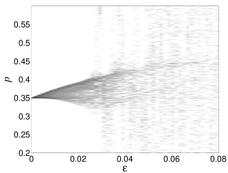
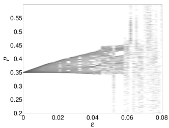
Figure 4: Distribution of momentum $p$ as a function of $\varepsilon$ for Hamiltonian (7) with the approximate control term (12) containing an error of $\delta\omega=0.001$ in the frequency (left panel) and an error of $\delta\varphi=0.2$ in the phase (right panel). The numerical results are obtained for the same values of the parameters as in Fig. 2.

In summary, we have shown here how our method of control works in suppressing chaotic velocity diffusion induced in a cold electron beam interacting with electrostatic waves. These numerical results have been successfully confirmed by an experimental check performed on a Traveling Wave Tube TWT05 . According to the fact that if the amplitude of the potential is of order $\varepsilon$ then the amplitude of the control term is of order $\varepsilon^{2}$, the control term is realized with an additional cost of energy that is less than $0.1\%$ of the initial electrostatic energy of the two wave system.

3 Acknowledgements

We acknowledge useful discussions with F. Doveil, Y. Elskens, Ph. Ghendrih and A. Macor. We acknowledge the financial support from Euratom/CEA (contract EUR 344-88-1 FUA F).

References

- (1) W. Scandale and G. Turchetti, Nonlinear Problems in Future Particle Accelerators (World Scientific, Singapore, 1991).
- (2) C. Steier, D. Robin, L. Nadolski, W. Decking, Y. Wu and J. Laskar, Phys. Rev. E 65 (2002) 056506.
- (3) R. Bonifacio, F. Casagrande, G. Cerchioni, L. De Salvo Souza, P. Pierini and N. Piovella, Riv. Nuovo Cim. 13 (1990) 1.
- (4) G. De Ninno and D. Fanelli, Phys. Rev. Lett. 92 (2004) 094801.
- (5) B.A. Carreras, IEEE Trans. Plasma Sci. 25 (1997) 1281.
- (6) A rather extended list of references on controlling chaos can be found in G. Chen and X. Dong From Chaos to Order (World Scientific, Singapore, 1998), and in D.J. Gauthier, Am. J. Phys. Resource Letter section 71 (2003) 750.
- (7) B.V. Chirikov, Phys. Rep. 52 (1979) 263.
- (8) M. Vittot, C. Chandre, G. Ciraolo and R. Lima, Nonlinearity 18 (2005) 423.
- (9) C. Chandre, M. Vittot, G. Ciraolo, Ph. Ghendrih and R. Lima, Nuclear Fusion (2005) to appear.
- (10) C. Chandre and H.R. Jauslin, Phys. Rep. 365 (2002) 1.
- (11) C. Chandre, G. Ciraolo, F. Doveil, R. Lima, A. Macor and M. Vittot, Phys. Rev. Lett. 94 (2005) 074101.