Abstract

Model of a passive scalar field advected by the compressible Gaussian strongly anisotropic velocity field with the covariance $\propto\delta(t-t^{\prime})|{\bf x}-{\bf x^{\prime}}|^{2\varepsilon}$ is studied by using the field theoretic renormalization group and the operator product expansion. The inertial-range stability of the corresponding scaling regime is established. The anomalous scaling of the single-time structure functions is studied and the corresponding anomalous exponents are calculated. Their dependence on the compressibility parameter and anisotropy parameters is analyzed. It is shown that, as in the isotropic case, the presence of compressibility leads to the decreasing of the critical dimensions of the important composite operators, i.e., the anomalous scaling is more pronounced in the compressible systems. All calculations are done to the first order in $\varepsilon$.

PACS numbers: 47.10.+g; 47.27.-i

Keywords: Passive scalar; Renormalization group; Anomalous scaling

1 Introduction

During the last two decades the so-called ”rapid change model” of a passively advected scalar by a self-similar Gaussian $\delta-$correlated in time velocity field introduced by Kraichnan [1] and number of its extensions have played the central role in the theoretical investigation of intermittency and anomalous scaling, the problems which stay in the center of attention in the framework of the inertial range investigation of fully developed turbulence [2, 3], i.e., in the range characterized by the scales which are far away from the largest scales at which energy is pumping into the system and, at the same time, far away form the smallest scales which are related to the dissipation processes. There are at least three reasons for this interest: First of all, it is well-known from experimental and also theoretical studies that the deviations from the statements of the famous classical Kolmogorov-Obukhov phenomenological theory (see, e.g., [2, 4, 5]) is surprisingly more noticeable and visible for the simpler models of passively advected scalar quantity (scalar field) than for the velocity field itself (see, e.g., [6, 7, 8, 9, 10, 11]); second, at the same time, the problem of passive advection of scalar field (as well as vector field) is much easier from theoretical point of view than the original problem of anomalous scaling in the framework of Navier-Stokes velocity field, and, in the end, third, even very simplified models with given Gaussian statistics of velocity field lead to the anomalous behavior which describe many features of the real turbulent advection, see, e.g., Refs. [1, 8, 9, 10, 11, 12, 13, 14, 15, 16, 17, 18] and references cited therein. As was already mentioned, the crucial role in these studies was played (and is still played) by the aforementioned rapid change model of a passive scalar advection, where, for the first time, the systematic analysis of the corresponding anomalous exponents was done on the microscopic level. For example, within the so-called ”zero-mode approach” to the rapid change model [12] (see also survey paper [19]) the anomalous exponents are found from the homogenous solutions (zero modes) of the closed equations for the single-time correlations.

On the other hand, one of the most effective approach for studying self-similar scaling behavior is the method of the field theoretic renormalization group (RG) [20, 21]. It can be also used in the theory of fully developed turbulence [22, 23] and related problems, e.g., in the problem of a passive scalar advection by the turbulent environment [24] (see also Refs. [21, 25, 26] for details).

In Refs. [27] the field theoretic RG and operator-product expansion (OPE) were used in the systematic investigation of the rapid-change model of a passive scalar. It was shown that within the field theoretic approach the anomalous scaling is related to the very existence of so-called ”dangerous” composite operators with negative critical dimensions in OPE (see, e.g., Refs. [21, 26] for details). In the subsequent papers [28] the anomalous exponents of the model were calculated within the $\varepsilon$ expansion up to order $\varepsilon^{3}$ (three-loop approximation). Here $\varepsilon$ is a parameter which describes a given equal-time pair correlation function of the velocity field (see next section). Important advantages of the RG approach are its universality and calculational efficiency: a regular systematic perturbation expansion for the anomalous exponents was constructed, similar to the well-known $\epsilon$-expansion in the theory of phase transitions.

Besides various generalizations of the Kraichnan model towards more realistic ones, namely, models with inclusion of small scale anisotropy [29], compressibility [30, 31], and finite correlation time of the velocity field [32, 33, 34] were studied by the field theoretic approach. General conclusion of all these investigations is that the anomalous scaling, which is the most intriguing and important feature of the Kraichnan rapid change model, remains valid for all generalized models.

In Ref. [29] the field theoretic RG and OPE were applied to the rapid change model of passive scalar advected by Gaussian strongly anisotropic velocity field where the anomalous exponents of the structure functions were calculated to the first order in $\varepsilon$ expansion. It was shown that in the presence of small-scale anisotropy the corresponding exponents are nonuniversal, i.e., they are functions of the anisotropy parameters, and they form the hierarchy with the leading exponent related to the most ”isotropic” operator. The importance of these investigations is related to the question of the influence of anisotropy on inertial-range behavior of passively advected fields as well as the velocity field itself [13, 14, 32, 33, 35, 36, 37, 38, 39, 40] (see also the survey paper [41] and references cited therein, as well as recent astrophysical investigations, e.g, in Refs. [42, 43]). On one hand, it was shown that for the even structure (or correlation) functions the exponents which describe the inertial-range scaling exhibit universality and they are ordered hierarchically in respect to degree of anisotropy with leading contribution given by the exponent from the isotropic shell but, on the other hand, the survival of the anisotropy in the inertial-range is demonstrated by the behavior of the odd structure functions, namely, the so-called skewness factor decreases down the scales slower than expected earlier in accordance with the classical Kolmogorov-Obukhov theory.

On the other hand, in Ref. [31] the influence of compressibility and large-scale anisotropy on the anomalous scaling behavior was studied in the aforementioned model in the order $\varepsilon^{2}$ in the $\varepsilon$ expansion, and anomalous exponents of higher-order correlation functions were calculated as functions of the parameter of compressibility. It was shown that the exponents exhibit hierarchy related to the degree of anisotropy. Again, the existence of small-scale anisotropy effects were demonstrated by the odd dimensionless ratios of correlation functions: the skewness and hyperskewness factors, and it was shown that the persistent of small-scale anisotropy is more pronounced for larger values of the compressibility parameter $\alpha$. From this point of view, compressible systems are very interesting to be studied.

In present paper, we shall continue in the investigation of the model, namely, for the first time, we shall study the model with compressible velocity field together with assumption about its small-scale uniaxial anisotropy in the first order in $\varepsilon$, i.e., we shall extend the model studied in Ref. [29] to the compressible case. In this situation, in general, two types of diffusion-advection problems of scalar particles exist in the compressible case which are identical in the incompressible case. In what follows, we shall study only one of them, namely, the advection of so-called ”tracer” (see, e.g., Ref.  [31]), i.e., for example, concentration of a scalar impurity, temperature, entropy, etc. Details will be shown in the next section.

First of all we shall establish stability of the scaling regime of the model and coordinates of the corresponding infrared (IR) stable fixed point will be found analytically as functions of the compressibility and anisotropy parameters. These results will be then used in the analysis of the asymptotic behavior of the single-time structure functions of a passively advected scalar field.

The paper is organized as follows: In Sec. 2 we present definition of the model and introduce the compressibility and small-scale uniaxial anisotropy to the given pair correlation function of the velocity field. In Sec. 3 we give the field theoretic formulation of the original stochastic problem and discuss the corresponding diagrammatic technique. The analysis of the ultraviolet (UV) divergences of the model is given, the multiplicative renormalizability of the model is established, and the renormalization constants are calculated in one-loop approximation. In Sec. 4 we analyze infrared (IR) asymptotic behavior of the model which is governed by the IR stable fixed point. Explicit expressions for the coordinates of the IR fixed point are found. In Sec. 5 the renormalization of needed composite operators is done and their critical dimensions are found as functions of parameters of the model. In Sec. 6 discussion of results is present.

2 The model of advection of passive ”tracer”

We shall consider the problem of the advection of a passive ”tracer” $\theta(x)\equiv\theta(t,{\bf x})$ which is described by the following stochastic equation

$$\partial_{t}\theta=\nu_{0}\triangle\theta-(v_{i}\partial_{i})\theta+f,$$ (1)

where $\partial_{t}\equiv\partial/\partial t$, $\partial_{i}\equiv\partial/\partial x_{i}$, $\triangle\equiv\partial^{2}$ is the Laplace operator, $\nu_{0}$ is the coefficient of molecular diffusivity (hereafter all parameters with a subscript $0$ denote bare parameters of unrenormalized theory; see below), $v_{i}\equiv v_{i}(x)$ is the $i$-th component of the compressible velocity field ${\bf v}(x)$, and $f\equiv f(x)$ is a Gaussian random noise with zero mean and correlation function

$$D^{f}\equiv\langle f(x)f(x^{\prime})\rangle=\delta(t-t^{\prime})C({\bf r}/L),\,\,\,{\bf r}={\bf x}-{\bf x^{\prime}},$$ (2)

where parentheses $\langle...\rangle$ hereafter denote average over corresponding statistical ensemble. The noise defined in Eq. (2) maintains the steady-state of the system but the concrete form of the correlator will not be essential in what follows. The only condition which must be fulfilled by the function $C({\bf r}/L)$ is that it must decrease rapidly for $r\equiv|{\bf r}|\gg L$, where $L$ denotes an integral scale related to the stirring.

As was already mentioned in Introduction, another type of the diffusion-advection problem exists in the case when compressibility of the velocity field is supposed which is given by the following more general stochastic equation [31, 44]

$$\partial_{t}\theta=\nu_{0}\triangle\theta-\partial_{i}(v_{i}\theta)+f.$$ (3)

It describes the passive advection of a density field but, in what follows, we shall not study this problem. In the case of incompressible velocity field (it is given mathematically by the divergence-free condition $\partial_{i}v_{i}=0$) both models are equivalent.

In real problems it is traditionally assumed that the velocity field ${\bf v}(x)$ satisfies stochastic Navier-Stokes equation [24]. In spite of, in what follows, we shall suppose that the velocity field obeys a Gaussian distribution with zero mean and two-point correlator

$$\langle v_{i}(x)v_{j}(x^{\prime})\rangle\equiv D^{v}_{ij}(x;x^{\prime})=D_{0}\delta(t-t^{\prime})\int\frac{d^{d}k}{(2\pi)^{d}}\frac{R_{ij}({\bf k})}{(k^{2}+m^{2})^{d/2+\varepsilon}}\exp[i{\bf k}({\bf x}-{\bf x^{\prime}})],$$ (4)

i.e, we shall work in the framework of the so-called rapid-change model [1, 12, 17, 18, 27, 28, 29, 30, 45, 46, 47]. Here, $d$ denotes the dimension of the ${\bf x}$ space, and $D_{0}$ is an amplitude factor related to the coupling constant $g_{0}$ of the model (expansion parameter in the perturbation theory, see next Section) by the relation $D_{0}/\nu_{0}\equiv g_{0}\simeq\Lambda^{2\varepsilon}$, where $\Lambda$ is the characteristic UV momentum scale. The parameter of the energy spectrum of the velocity field $0<\varepsilon<1$ is taken in such a way that its ”Kolmogorov” value (the value which corresponds to the Kolmogorov scaling of the velocity correlation function in developed turbulence) is $\varepsilon=2/3$, and $1/m$ is another integral scale. In general, the scale $1/m$ may be different from the integral scale $L$ introduced in Eq. (2) but, in accordance with Ref. [29], we suppose that $1/m\simeq L$.

In the incompressible isotropic case the second-rank tensor $R_{ij}({\bf k})$ in Eq. (4) has the simple form of the ordinary transverse projector $R_{ij}({\bf k})=P_{ij}({\bf k})\equiv\delta_{ij}-k_{i}k_{j}/k^{2}$, where $k=|{\bf k}|$. This tensor is changed when one incorporates small-scale anisotropy or compressibility. Let us briefly discuss these questions.

First of all, in the case of incompressible anisotropic case a new second-rank tensor must be again a transverse operator because the velocity field is still divergence-free ($\partial_{i}v_{i}=0$). The simplest way how to introduce small-scale uniaxial anisotropy is to take the operator $R_{ij}({\bf k})$ in the following way [29]

$$R_{ij}({\bf k})=\left(1+\alpha_{1}\frac{({\bf n\cdot k})^{2}}{k^{2}}\right)P_{ij}({\bf k})+\alpha_{2}n_{s}n_{l}P_{is}({\bf k})P_{jl}({\bf k})\,,$$ (5)

where $P_{ij}({\bf k})$ is the usual transverse projection operator (as defined above), the unit vector ${\bf n}$ determines the distinguished direction, and $\alpha_{1}$, $\alpha_{2}$ are parameters characterizing the anisotropy. The positive definiteness of the correlation function (4) imposes the following restrictions on their values: $\alpha_{1}\,,\alpha_{2}>-1$. The operator (5) is a special case of the general transverse structure that possesses uniaxial anisotropy:

$$R_{ij}({\bf k})=a(\psi)P_{ij}({\bf k})+b(\psi)n_{s}n_{l}P_{is}({\bf k})P_{jl}({\bf k})\,,$$ (6)

where $\psi$ denotes the angle between the vectors ${\bf n}$ and ${\bf k}$ (${\bf n\cdot k}=k\cos\psi$). Using Gegenbauer polynomials [48] the scalar functions in representation (6) may be expressed in the form

$$a(\psi)=\sum_{i=0}^{\infty}a_{i}P_{2i}(\cos\psi)\,,\,\,\,\,b(\psi)=\sum_{i=0}^{\infty}b_{i}P_{2i}(\cos\psi)\,.$$

It was shown in Ref. [29] that all main features of the general model with the anisotropy structure represented by Eq. (6) are included in the simplified model with the special form of the transverse operator given by Eq. (5).

Second, in the case of the compressible isotropic velocity field the second-rank tensor $R_{ij}({\bf k})$ in Eq. (4) is not longer a transverse projector but it is rather a combination of the transverse projector $P_{ij}({\bf k})\equiv\delta_{ij}-k_{i}k_{j}/k^{2}$ and of the longitudinal projector $Q_{ij}({\bf k})\equiv k_{i}k_{j}/k^{2}$ as a result of the fact that the velocity field is not longer solenoidal one. Thus, in this case, the correlator (4) contains the tensor structure of the following general form

$$R_{ij}({\bf k})=P_{ij}({\bf k})+\alpha Q_{ij}({\bf k})$$ (7)

where $\alpha\geq 0$ is a free parameter of the compressibility. The value $\alpha=0$ corresponds to the divergence-free (incompressible) advecting velocity field. It was used in Refs. [30, 31] for determination of the influence of the compressibility on the anomalous scaling of the correlation functions of scalar density, as well as tracer fields in two-loop level.

In what follows, we shall study the combined effects given by the small-scale anisotropy and compressibility and our aim will be to study possible deviations from the conclusions given in Ref. [29], where the rapid-change model of passively advected scalar field with small scale uniaxial anisotropy was studied. To do this, it is necessary to introduce into the velocity field correlator (4) corresponding second-rank tensor which will have needed properties. The simplest way how to do this is to add longitudinal projector $Q_{ij}({\bf k})\equiv k_{i}k_{j}/k^{2}$ to the uniaxial anisotropic transverse tensor structure given in Eq. (5). Thus, the result tensor structure which will be used in our investigations is defined as

$$R_{ij}({\bf k})=P_{ij}({\bf k})+\alpha Q_{ij}({\bf k})+\alpha_{1}\frac{({\bf n\cdot k})^{2}}{k^{2}}P_{ij}({\bf k})+\alpha_{2}n_{s}n_{l}P_{is}({\bf k})P_{jl}({\bf k})\,.$$ (8)

It means that we have introduced the compressible term to the isotropic component of the axially anisotropic tensor structure (5) only. Therefore, the contributions of compressibility and anisotropy are given by a simple sum of the corresponding terms. Nevertheless, as we shall see, the combined effects of anisotropy and compressibility on the results will not be a simple sum of them.

3 Field Theoretic Formulation of the Model, UV Renormalization and RG analysis

According to the well-known general theorem (see, e.g., Refs.[20, 21]) the stochastic problem (1) and (2) is equivalent to the field-theoretic model of the set of three fields $\Phi\equiv\{\theta,\theta^{\prime},{\bf v}\}$ with the following action functional

$$S(\Phi) = -\frac{1}{2}\int dt_{1}\,d^{d}{\bf x_{1}}\,dt_{2}\,d^{d}{\bf x_{2}}\,v_{i}(t_{1},{\bf x_{1}})[D_{ij}^{v}(t_{1},{\bf x_{1}};t_{2},{\bf x_{2}})]^{-1}v_{j}(t_{2},{\bf x_{2}})$$ (9)

$$+\frac{1}{2}\int dt_{1}\,d^{d}{\bf x_{1}}\,dt_{2}\,d^{d}{\bf x_{2}}\,\theta^{\prime}(t_{1},{\bf x_{1}})D^{f}(t_{1},{\bf x_{1}};t_{2},{\bf x_{2}})\theta^{\prime}(t_{2},{\bf x_{2}})$$

$$+\int dt\,d^{d}{\bf x}\,\,\theta^{\prime}\left[-\partial_{t}-v_{i}\partial_{i}+\nu_{0}\triangle\right]\theta,$$

where $\theta^{\prime}$ is an auxiliary field, and all summations over the vector indices are implied. The second and the third integral in Eq. (9) correspond to the Martin-Siggia-Rose action [49] for the stochastic problem (1), (2) at fixed velocity field ${\bf v}$, and the first integral describes the Gaussian averaging over ${\bf v}$ defined by the correlator $D^{v}$ in Eq. (4) with tensor $R_{ij}({\bf k})$ given in Eq. (8).

Action (9) is given in a form convenient for application of the field theoretic perturbation analysis with the standard Feynman diagrammatic technique. From the quadratic part of the action one obtains the matrix of bare propagators. The wave-number-frequency representation of propagators of the fields $\theta$ and $\theta^{\prime}$ is

$$\langle\theta\theta^{\prime}\rangle_{0} = \langle\theta^{\prime}\theta\rangle^{*}_{0}=\frac{1}{-i\omega+\nu_{0}k^{2}},$$ (10)

$$\langle\theta\theta\rangle_{0} = \frac{C({\bf k})}{(-i\omega+\nu_{0}k^{2})(i\omega+\nu_{0}k^{2})},$$ (11)

$$\langle\theta^{\prime}\theta^{\prime}\rangle_{0} = 0$$ (12)

where $C({\bf k})$ is the Fourier transform of the function $C({\bf r}/L)$ form Eq. (2). On the other hand, the bare propagator of the velocity field $\langle vv\rangle_{0}$ is defined by Eq. (4) with the tensor structure given by Eq. (8). In what follows, we shall need only the propagators $\langle\theta\theta^{\prime}\rangle_{0}$ and $\langle vv\rangle_{0}$. Their graphical representation is shown in Fig. 1. The interaction in the model is given by the nonlinear term $-\theta^{\prime}(v_{i}\partial_{i})\theta=\theta^{\prime}v_{j}V_{j}\theta$ with the vertex factor which in the wave-number-frequency representation has the form (the momentum flows into the vertex via the scalar field $\theta$):

$$V_{j}=-ik_{j}.$$ (13)

Its graphical representation is given in Fig. 1.

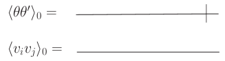
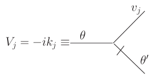
Figure 1: (Left) The graphical representation of needed propagators of the model. (Right) The interaction vertex of the model (wave-number-frequency representation). The momentum flows into the vertex via the scalar field $\theta$.

Standard power counting [20, 21] leads to the identification of correlation functions with superficial UV divergences. In the framework of the rapid-change passive advection models detail analysis of this question was done, e.g., in Ref. [29], where it was shown that the only one-particle-irreducible (1PI) Green function which possesses superficial UV-divergences is the function $\Gamma_{\theta^{\prime}\theta}\equiv\langle\theta^{\prime}\theta\rangle_{1-ir}$ (within the rapid-change model the situation is unchanged when compressibility of the system is assumed) and, in the isotropic case, this Green function leads only to the renormalization of the term $\nu_{0}\theta^{\prime}\triangle\theta$ of action (9) and the corresponding UV divergences may be fully absorbed in the adequate redefinition of the existing parameters $g_{0}$, $\nu_{0}$. Thus, all correlation functions calculated in terms of the renormalized parameters $g,\nu$ are UV finite.

The situation becomes, however, more complicated when anisotropy is introduced. It is related to the fact that in this case the 1PI Green function $\Gamma_{\theta^{\prime}\theta}$ contains divergences corresponding to the structure $\theta^{\prime}({\bf n}\cdot{\bf\partial})^{2}\theta$ (the only possible anisotropic structure $\sim\triangle\equiv\partial^{2}$) which is not present in original unrenormalized action (9). It leads to the non-renormalizability of the model in the anisotropic case. To make the model multiplicatively renormalizable it is necessary to extend original action (9) by including needed term with corresponding new parameter. As a result the extended model is described by the following action

$$S(\Phi) = -\frac{1}{2}\int dt_{1}\,d^{d}{\bf x_{1}}\,dt_{2}\,d^{d}{\bf x_{2}}\,v_{i}(t_{1},{\bf x_{1}})[D_{ij}^{v}(t_{1},{\bf x_{1}};t_{2},{\bf x_{2}})]^{-1}v_{j}(t_{2},{\bf x_{2}})$$

$$+\frac{1}{2}\int dt_{1}\,d^{d}{\bf x_{1}}\,dt_{2}\,d^{d}{\bf x_{2}}\,\theta^{\prime}(t_{1},{\bf x_{1}})D^{f}(t_{1},{\bf x_{1}};t_{2},{\bf x_{2}})\theta^{\prime}(t_{2},{\bf x_{2}})$$

$$+\int dt\,d^{d}{\bf x}\theta^{\prime}\left[-\partial_{t}-v_{i}\partial_{i}+\nu_{0}\triangle+\chi_{0}\nu_{0}({\bf n}\cdot{\bf\partial})^{2}\right]\theta,$$

where a new unrenormalized parameter $\chi_{0}$ has been introduced. As was pointed out in Ref. [29] the stability of the system requires the positivity of the total viscous contribution $\nu_{0}k^{2}+\chi_{0}\nu_{0}({\bf n}\cdot{\bf k})^{2}$, i.e., the inequality $\chi_{0}>-1$ must be fulfilled. This modification leads, of course, also to the modification of the corresponding isotropic propagators of the fields $\theta,\theta^{\prime}$ given in Eqs. (10) and (11) which are now defined as (see also Ref. [29])

$$\langle\theta\theta^{\prime}\rangle_{0}=\langle\theta^{\prime}\theta\rangle^{*}_{0} = \frac{1}{-i\omega+\nu_{0}k^{2}+\chi_{0}\nu_{0}({\bf n}\cdot{\bf k})^{2}},$$ (15)

$$\langle\theta\theta\rangle_{0} = \frac{C({\bf k})}{|-i\omega+\nu_{0}k^{2}+\chi_{0}\nu_{0}({\bf n}\cdot{\bf k})^{2}|^{2}}.$$ (16)

After this modifications the model defined by action (3) becomes multiplicatively renormalizable and the standard RG analysis can be now applied. The corresponding renormalized action has the form

$$S^{R}(\Phi) = -\frac{1}{2}\int dt_{1}\,d^{d}{\bf x_{1}}\,dt_{2}\,d^{d}{\bf x_{2}}\,v_{i}(t_{1},{\bf x_{1}})[D_{ij}^{v}(t_{1},{\bf x_{1}};t_{2},{\bf x_{2}})]^{-1}v_{j}(t_{2},{\bf x_{2}})$$

$$+\frac{1}{2}\int dt_{1}\,d^{d}{\bf x_{1}}\,dt_{2}\,d^{d}{\bf x_{2}}\,\theta^{\prime}(t_{1},{\bf x_{1}})D^{f}(t_{1},{\bf x_{1}};t_{2},{\bf x_{2}})\theta^{\prime}(t_{2},{\bf x_{2}})$$

$$+\int dt\,d^{d}{\bf x}\theta^{\prime}\left[-\partial_{t}-v_{i}\partial_{i}+\nu Z_{1}\triangle+\chi\nu Z_{2}({\bf n}\cdot{\bf\partial})^{2}\right]\theta,$$

where $Z_{1}$ and $Z_{2}$ are the renormalization constants (they absorb the UV divergent parts of the 1PI function $\Gamma_{\theta^{\prime}\theta}$). It is equivalent to the multiplicative renormalization of the bare parameters $g_{0},\nu_{0}$, and $\chi_{0}$, namely

$$\nu_{0}=\nu Z_{\nu},\quad g_{0}=g\mu^{2\varepsilon}Z_{g},\quad\chi_{0}=\chi Z_{\chi},$$ (18)

where $g,\nu$, and $\chi$ are renormalized counterparts of the corresponding bare parameters, and $\mu$ is a scale setting parameter or the reference mass (it has the same canonical dimension as the wave number). In what follows, we shall work in minimal subtraction scheme (MS), therefore, in one-loop approximation, the renormalization constants $Z$ have the form $1+A(g,\alpha,\chi,\alpha_{1},\alpha_{2},d)/\varepsilon$. Thus, $A$ is a function of dimensionless parameters but it is independent of $\varepsilon$.

By comparison of the corresponding terms in action (3) with definitions of the renormalization constants $Z$ for parameters (18), one obtains the following relations between renormalization constants:

$$Z_{\nu}=Z_{1},\quad Z_{\chi}=Z_{2}Z_{1}^{-1},\quad Z_{g}=Z_{1}^{-1},$$ (19)

where last relation in Eq. (19) is a consequence of the fact that $D_{0}$ defined in Eq. (4) is not renormalized, i.e., $D_{0}=g_{0}\nu_{0}=g\nu\mu^{2\varepsilon}$.

Standardly, the formulation through the action functional (9) (or through (3) in the anisotropic case) replaces the statistical averages of random quantities in the stochastic problem defined by Eqs. (1) and (2) with equivalent functional averages with weight $\exp S(\Phi)$. Generating functionals of total Green functions G(A) and connected Green functions W(A) are then defined by the functional integral

$$G(A)=e^{W(A)}=\int{\cal D}\Phi\,\,e^{S(\Phi)+A\Phi},$$ (20)

where $A(x)=\{A^{\theta},A^{\theta^{\prime}},{\bf A^{v}}\}$ represents a set of arbitrary sources for the set of fields $\Phi$, ${\cal D}\Phi\equiv{\cal D}\theta{\cal D}\theta^{\prime}{\cal D}{\bf v}$ denotes the measure of functional integration, and linear form $A\Phi$ is defined as

$$A\Phi=\int d\,x[A^{\theta}(x)\theta(x)+A^{\theta^{\prime}}(x)\theta^{\prime}(x)+A_{i}^{v}(x)v_{i}(x)].$$ (21)

Let us continue with renormalization of the model. The relation $S(\theta,\theta^{\prime},{\bf v},e_{0})=S^{R}(\theta,\theta^{\prime},{\bf v},e,\mu)$, where $e_{0}$ stands for the complete set of bare parameters and $e$ stands for renormalized one, leads to the relation $W(A,e_{0})=W^{R}(A,e,\mu)$ for the generating functional of connected Green functions. By application of the operator $\tilde{\cal{D}}_{\mu}\equiv\mu\partial_{\mu}$ at fixed $e_{0}$ on both sides of the latest equation one obtains the basic RG differential equation

$${\cal{D}}_{RG}W^{R}(A,e,\mu)=0,$$ (22)

where ${\cal{D}}_{RG}$ represents operation $\tilde{\cal{D}}_{\mu}$ written in the renormalized variables. Its explicit form is

$${\cal{D}}_{RG}={\cal{D}}_{\mu}+\beta_{g}(g,\chi)\partial_{g}+\beta_{\chi}(g,\chi)\partial_{u}-\gamma_{\nu}(g,\chi){\cal{D}}_{\nu},$$ (23)

where we denote ${\cal{D}}_{x}\equiv x\partial_{x}$ for any variable $x$ and the RG functions (the $\beta$ and $\gamma$ functions) are given by well-known definitions (see, e.g., Refs. [20, 21]) and, in our case, by using relations (19) for renormalization constants, they have the following form

$$\gamma_{i} \equiv \tilde{\cal{D}}_{\mu}\ln Z_{i},\,\,\,i=1,2$$ (24)

$$\beta_{g} \equiv \tilde{\cal{D}}_{\mu}g=g(-2\varepsilon+\gamma_{1}),$$ (25)

$$\beta_{\chi} \equiv \tilde{\cal{D}}_{\mu}\chi=\chi(\gamma_{1}-\gamma_{2}).$$ (26)

The renormalization constants $Z_{1,2}$ are determined by the requirement that the one-particle irreducible Green function $\langle\theta^{\prime}\theta\rangle_{1-ir}$ must be UV finite when is written in renormalized variables. In our case it means that they have no singularities in the limit $\varepsilon\rightarrow 0$. The one-particle irreducible Green function $\langle\theta^{\prime}\theta\rangle_{1-ir}$ is related to the self-energy operator $\Sigma_{\theta^{\prime}\theta}$ by the Dyson equation

$$\langle\theta^{\prime}\theta\rangle_{1-ir}=-i\omega+\nu_{0}p^{2}+\nu_{0}\chi_{0}({\bf n}\cdot{\bf p})^{2}-\Sigma_{\theta^{\prime}\theta}(\omega,p).$$ (27)

Thus $Z_{1,2}$ are found from the requirement that the UV divergences are canceled in Eq. (27) after substitutions $\nu_{0}=\nu Z_{1}$ and $\nu_{0}\chi_{0}=\nu\chi Z_{2}$. This determines $Z_{1,2}$ up to an UV finite contributions, which are fixed by the choice of the renormalization scheme. In the MS scheme, as was mentioned already above, all the renormalization constants have the form: 1 + pole in $\varepsilon$. In one-loop approximation the self-energy operator $\Sigma_{\theta^{\prime}\theta}$ is represented by the corresponding one-particle irreducible diagram which is shown in Fig. 2 but it must be stressed that, at the same time, it is an exact result because in rapid-change model all higher-loop diagrams contain at least one closed loop which is built on by retarded or advanced propagators only, thus they are automatically equal to zero.

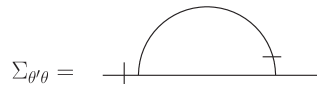
Figure 2: The only diagram which contribute to the self-energy operator $\Sigma_{\theta^{\prime}\theta}$.

The diagram in Fig. 2 has the following analytical representation

$$\Sigma_{\theta^{\prime}\theta}=-\frac{S_{d}}{(2\pi)^{d}}\frac{g\nu}{4}\left(\frac{\mu}{m}\right)^{2\varepsilon}\frac{1}{\varepsilon}(p^{2}A_{1}+({\bf p}\cdot{\bf n})^{2}A_{2})\,,$$ (28)

where $S_{d}=2\pi^{d/2}/\Gamma(d/2)$ denotes the d-dimensional sphere, and the functions $A_{1}$ and $A_{2}$ have the following simple explicit form

$$A_{1} = \frac{(d+2)(d-1+\alpha)+\alpha_{1}(d+1)+\alpha_{2}}{d(d+2)},$$ (29)

$$A_{2} = \frac{-2(\alpha_{1}+\alpha_{2})+d^{2}\alpha_{2}}{d(d+2)},$$ (30)

In the end, the renormalization constants $Z_{1}$ and $Z_{2}$ are given as follows

$$Z_{1}=1-\frac{g}{\varepsilon}\frac{S_{d}}{(2\pi)^{d}}\frac{A_{1}}{4}\,,$$ (31)

$$Z_{2}=1-\frac{g}{\varepsilon}\frac{S_{d}}{(2\pi)^{d}}\frac{A_{2}}{4\chi}\,.$$ (32)

Because of the second rank tensor (8) is taken in the simple form of the sum of the uniaxial anisotropic transverse projector and the longitudinal projector then, as a result of this fact, the self-energy operator $\Sigma_{\theta^{\prime}\theta}$ is also a simple sum of the results obtained in Refs. [29] and [31]. Using the definition of anomalous dimensions $\gamma_{1,2}$ in Eq. (24) one comes to the following expressions

$$\gamma_{1}=\frac{\bar{g}}{2}A_{1}\,,\quad\gamma_{2}=\frac{\bar{g}}{2\chi}A_{2},$$ (33)

where we denote $\bar{g}=gS_{d}/(2\pi)^{d}$, and $A_{1,2}$ are given in Eqs. (29) and (30).

Let us note once more that the expressions (31)-(33) are exact as a result of non-existence of the higher-loop corrections.

4 Fixed point and scaling regime

Possible scaling regimes of a renormalizable model are directly given by the IR stable fixed points of the corresponding system of RG equations [20, 21]. The fixed point of the RG equations is defined by $\beta$-functions, namely, by requirement of their vanishing. In our model, the coordinates $g_{*},\chi_{*}$ of a fixed point are found from the system of two equations

$$\beta_{g}(g_{*},\chi_{*})=\beta_{\chi}(g_{*},\chi_{*})=0.$$ (34)

The beta functions $\beta_{g}$ and $\beta_{\chi}$ are defined in Eqs. (25), and (26). To investigate the IR stability of a fixed point it is enough to analyze the eigenvalues of the matrix $\Omega$ of the first derivatives:

$$\Omega_{ij}=\left(\begin{array}[]{cc}\partial\beta_{g}/\partial g&\partial\beta_{g}/\partial\chi\\ \partial\beta_{\chi}/\partial g&\partial\beta_{\chi}/\partial\chi\end{array}\right).$$ (35)

The IR asymptotic behavior is governed by the IR stable fixed points, i.e., those for which both eigenvalues are positive. Using the explicit expressions given in Eq. (33) together with the definitions of $\beta$ functions in Eqs. (25) and (26) leads to the explicit expressions for the coordinates of the non-trivial IR stable fixed point

$$\bar{g}_{*} = \frac{4d(d+2)\varepsilon}{(d+2)(d-1+\alpha)+\alpha_{1}(d+1)+\alpha_{2}},$$ (36)

$$\chi_{*} = \frac{-2(\alpha_{1}+\alpha_{2})+d^{2}\alpha_{2}}{(d+2)(d-1+\alpha)+\alpha_{1}(d+1)+\alpha_{2}}.$$ (37)

In the incompressible limit $\alpha\rightarrow 0$ one comes to the results of Ref. [29], namely

$$\bar{g}_{*}^{a} = \frac{4d(d+2)\varepsilon}{(d+2)(d-1)+\alpha_{1}(d+1)+\alpha_{2}},$$ (38)

$$\chi_{*}^{a} = \frac{-2(\alpha_{1}+\alpha_{2})+d^{2}\alpha_{2}}{(d+2)(d-1)+\alpha_{1}(d+1)+\alpha_{2}}.$$ (39)

On the other hand, in isotropic limit $\alpha_{1,2}\rightarrow 0$ one has (see, e.g., Ref. [33])

$$\bar{g}_{*}^{c}=\frac{4d(d+2)\varepsilon}{(d+2)(d-1+\alpha)}.$$ (40)

Thus, as one can see, our definition of the second rank tensor (8) leads to the simple relation among $\bar{g}_{*},\bar{g}_{*}^{a}$, and $\bar{g}_{*}^{c}$, namely

$$\frac{1}{\bar{g}_{*}}=\frac{1}{\bar{g}_{*}^{a}}+\frac{1}{\bar{g}_{*}^{c}}.$$ (41)

The values of anomalous dimensions $\gamma_{1}$ and $\gamma_{2}$ are found exactly at fixed point and are defined as follows

$$\gamma_{1}^{*}=\gamma_{2}^{*}=2\varepsilon,$$ (42)

where $\gamma_{1,2}^{*}\equiv\gamma_{1,2}(g_{*},\chi_{*})$.

The matrix of the first derivatives taken at the fixed point has simple diagonal form

$$\Omega_{ij}=\left(\begin{array}[]{cc}2\varepsilon&0\\ 0&2\varepsilon\end{array}\right),$$ (43)

i.e., the fixed point is IR stable if $\varepsilon>0$. This is also the only condition to have $g_{*}>0$ (together, of course, with earlier discussed physical assumptions, namely: $\alpha_{1,2}>-1$ and $\alpha\geq 0$, see Sec. 2). The physical condition $\chi_{*}>-1$ is also fulfilled without further restrictions on the parameter space.

The issue of interest are especially multiplicatively renormalizable equal-time two-point quantities $G(r)$ (see, e.g., [29]). The example of such quantity are the equal-time structure functions

$$S_{N}(r)\equiv\langle[\theta(t,{\bf x})-\theta(t,{\bf x^{\prime}})]^{N}\rangle,\,\,r=|{\bf x}-{\bf x^{\prime}}|$$ (44)

in the inertial range specified by the inequalities $l\sim 1/\Lambda<<r<<L=1/m$ ($l$ is an internal length). Here parentheses $\langle\cdots\rangle$ mean functional average over fields $\Phi=\{\theta,\theta^{\prime},{\bf v}\}$ with weight $\exp S^{R}(\Phi)$.

First let us describe briefly IR scaling behavior in general on the example of an equal-time function $G(r)$ which is multiplicatively renormalizable. The IR scaling behavior of the function $G(r)$ (for $r/l\gg 1$ and any fixed $r/L$)

$$G(r)\simeq\nu_{0}^{d^{\omega}_{G}}l^{-d_{G}}(r/l)^{-\Delta_{G}}R(r/L)$$ (45)

is related to the existence of IR stable fixed points of the RG equations (see above). In Eq. (45) $d^{\omega}_{G}$ and $d_{G}$ are corresponding canonical dimensions of the function $G$: $d^{\omega}_{G}$ is the frequency dimension, and $d_{G}$ is the total canonical dimension. They are related by the relation $d_{G}=d_{G}^{k}+2d^{\omega}_{G}$, where $d_{G}^{k}$ is corresponding momentum canonical dimension. The existence of two independent canonical dimensions is related to the fact that our model belongs among two-scale dynamical models (details see, e.g., in Refs. [21, 26]). In Eq. (45) $R(r/L)$ is so-called scaling function which cannot be determined by RG equation (see, e.g., [21]), and $\Delta_{G}$ is the critical dimension defined as

$$\Delta_{G}=d_{G}^{k}+\Delta_{\omega}d_{G}^{\omega}+\gamma_{G}^{*}.$$ (46)

Here $\gamma_{G}^{*}$ is the fixed point value of the anomalous dimension $\gamma_{G}\equiv\mu\partial_{\mu}\ln Z_{G}$, where $Z_{G}$ is renormalization constant of multiplicatively renormalizable quantity $G$, i.e., $G=Z_{G}G^{R}$ [33], and $\Delta_{\omega}=2-\gamma_{\nu}^{*}=2-\gamma_{1}^{*}$ is the critical dimension of frequency with $\gamma_{1}^{*}=2\varepsilon$ as it is shown in Eq. (42).

Now, let us apply the above discussion to the inertial-range analysis of the equal-time structure functions as defined in Eq. (44). It is well-known that, in the isotropic case, the odd functions $S_{2n+1}$ vanish, while for $S_{2n}$ simple dimensional considerations give

$$S_{2n}(r)=\nu_{0}^{-n}\,r^{2n}\,R_{2n}(r/l,r/L),$$ (47)

where $R_{2n}$ are some functions of dimensionless variables. First, the multiplicative renormalizability of the model leads to the existence of differential RG equations for these structure functions and their asymptotic behavior for $r/l>>1$ and any fixed $r/L$ is given by IR stable fixed point of the RG equations and the structure functions can be written in the following form

$$S_{2n}(r)=\nu_{0}^{-n}\,r^{2n}\,(r/l)^{-\gamma_{n}}R_{2n}(r/L),\quad r/l>>1$$ (48)

with unknown scaling functions $R_{2n}(r/L)$. In the theory of critical phenomena [20, 21] the quantity $\gamma_{n}$ is known as “anomalous dimension” and $\Delta[S_{2n}]\equiv-2n+\gamma_{n}$ is termed the “critical dimension” (see above), where $-2n$ is the corresponding “canonical dimension”. In our case, $\gamma_{n}=2n\varepsilon$ [27], i.e., representation (48) implies the existence of a scaling in the IR region ($r/l>>1$, $r/L$ fixed) with definite critical dimensions of all “IR relevant” parameters, $\Delta[S_{2n}]=-2n(1-\varepsilon)$, $\Delta_{r}=-1$, $\Delta_{L^{-1}}=1$ and fixed “irrelevant” parameters $\nu_{0}$ and $l$ regardless of the form of the functions $R_{2n}(r/L)$.

The second stage of RG analysis is associated with the investigation of small $r/L$ behavior of the functions $R_{2n}(r/L)$ in Eq. (48) using the OPE. It shows that, in the limit $r/L\to 0$, the functions $R_{2n}(r/L)$ have the asymptotic form

$$R_{2n}(r/L)=\sum_{F}C_{F}(r/L)\,(r/L)^{\Delta_{n}},$$ (49)

where $C_{F}$ are some coefficients regular in $r/L$ and the summation is implied over certain renormalized composite operators $F$ with critical dimensions $\Delta_{n}$ [21]. In the case under consideration, the leading operators $F$ have the form $F_{n}=(\partial_{i}\theta\partial_{i}\theta)^{n}$. In Sec. 5 we shall consider them in detail where the complete calculation of the critical dimensions of the composite operators $F_{n}$ will be present for arbitrary values of $n$, $d$, $\alpha$ and $\alpha_{1,2}$.

5 Operator product expansion, Critical dimensions of composite operators, and Anomalous scaling

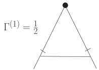
Figure 3: Graphical representation of the one-loop correction to the composite operator $\Gamma_{N}$ (details see in Ref. [29]).

5.1 Operator product expansion

Let us now study the behavior of the scaling function in Eq. (45). According to the OPE [20, 21, 25, 26], the equal-time product $F_{1}(x^{\prime})F_{2}(x^{\prime\prime})$ of two renormalized composite operators at ${\bf x}=({\bf x^{\prime}}+{\bf x^{\prime\prime}})/2=const$ and ${\bf r}={\bf x^{\prime}}-{\bf x^{\prime\prime}}\rightarrow 0$ can be written in the following form

$$F_{1}(x^{\prime})F_{2}(x^{\prime\prime})=\sum_{i}C_{F_{i}}({\bf r})F_{i}({\bf x},t),$$ (50)

where summation is taken over all possible renormalized local composite operators $F_{i}$ allowed by symmetry with definite critical dimensions $\Delta_{F_{i}}$, and the functions $C_{F_{i}}$ are the corresponding Wilson coefficients regular in $L^{-2}$. The renormalized correlation function $\langle F_{1}(x^{\prime})F_{2}(x^{\prime\prime})\rangle$ can be now found by averaging Eq. (50) with the weight $\exp S^{R}$ with $S^{R}$ from Eq. (3). The quantities $\langle F_{i}\rangle$ appear on the right-hand side, and their asymptotic behavior in the limit $L^{-1}\rightarrow 0$ is then found from the corresponding RG equations and has the form $\langle F_{i}\rangle\propto L^{-\Delta_{F_{i}}}$.

From the OPE (50) one can find that the scaling function $R(r/L)$ in the representation (45) for the correlation function $F_{1}(x^{\prime})F_{2}(x^{\prime\prime})$ has the form

$$R(r/L)=\sum_{i}C_{F_{i}}(r/L)^{\Delta_{F_{i}}},$$ (51)

where the coefficients $C_{F_{i}}$ are regular in $(r/L)^{2}$.

The principal feature of the turbulence models is the existence of the so-called ”dangerous” operators with negative critical dimensions [21, 25, 26, 27, 30]. Their presence in the OPE determines the IR behavior of the scaling functions and leads to their singular dependence on $L$ when $r/L\rightarrow 0$. Therefore, the turbulence models are crucially different from the models of critical phenomena, where the leading contribution to the representation (51) is given by the simplest operator $F=1$ with the dimension $\Delta_{F}=0$, and the other operators determine only the corrections that vanish for $r/L\rightarrow 0$.

Figure 4: Dependence of the critical dimension $\Delta[2,2]/\varepsilon$ on anisotropy parameters $\alpha_{1}$ ($\alpha_{2}=0$) and $\alpha_{2}$ ($\alpha_{1}=0$) for different values of the compressibility parameter $\alpha$.

If the spectrum of the dimensions $\Delta_{F_{i}}$ for a given scaling function is bounded from below, the leading term of its behavior for $r/L\rightarrow 0$ is given by the minimal dimension. It will be our case and for the investigation of the anomalous scaling of the structure functions (44) the leading contribution of the Taylor expansion is given by the tensor composite operators constructed solely of the scalar gradients (see, e.g., Ref. [29] for details)

$$F[N,p]\equiv\partial_{i_{1}}\theta\cdots\partial_{i_{p}}\theta(\partial_{i}\theta\partial_{i}\theta)^{n},$$ (52)

where $N=p+2n$ is the total number of the fields $\theta$ entering into the operator and $p$ is the number of the free vector indices.

Figure 5: (Left) Dependence of the critical dimension $\Delta[2,2]/\varepsilon$ on anisotropy parameters $\alpha_{1}=\alpha_{2}$ for different values of the compressibility parameter $\alpha$. (Right) Dependence of the critical dimension $\Delta[3,p]/\varepsilon,p=1,3$ on anisotropy parameter $\alpha_{1}$ ($\alpha_{2}=0$) for different values of the compressibility parameter $\alpha$.

5.2 Composite operators $F[N,p]$: renormalization and critical dimensions

Here we shall briefly discuss the renormalization of the composite operators (52) which play central role in our investigation (complete and detailed discussion of the renormalization of this composite operators can be found in Ref. [29]) but first we describe the basis of general theory.

Figure 6: Dependence of the critical dimension $\Delta[3,p]/\varepsilon,p=1,3$ on anisotropy parameters $\alpha_{2}$ ($\alpha_{1}=0$) and $\alpha_{1}=\alpha_{2}$ for different values of the compressibility parameter $\alpha$.

The necessity of additional renormalization of the composite operators (52) is related to the fact that the coincidence of the field arguments in Green functions containing them leads to additional UV divergences. These divergences must be removed by special kind of renormalization procedure which can be found, e.g., in Refs. [20, 21, 50], where their renormalization is studied in general. The renormalization of composite operators in the models of turbulence is discussed in Refs. [23, 26]. Besides, typically, the composite operators are mixed under renormalization.

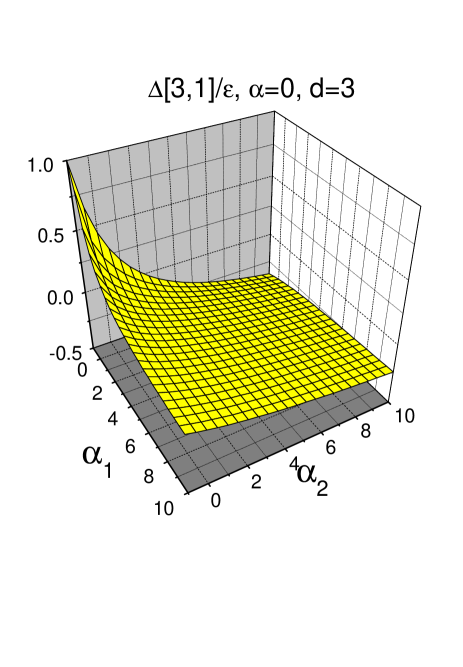
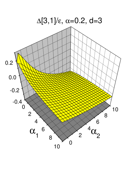
Figure 7: Behavior of the critical dimension $\Delta[3,1]/\varepsilon$ on anisotropy parameter $\alpha_{1}$ and $\alpha_{2}$ for $\alpha=0$ (incompressible case) and for $\alpha=0.2$.

Let $F\equiv\{F_{\alpha}\}$ be a closed set of composite operators which are mixed only with each other in renormalization. Then the renormalization matrix $Z_{F}\equiv\{Z_{\alpha\beta}\}$ and the matrix of corresponding anomalous dimensions $\gamma_{F}\equiv\{\gamma_{\alpha\beta}\}$ for this set are given as follows

$$F_{\alpha}=\sum_{\beta}Z_{\alpha\beta}F_{\beta}^{R},\qquad\gamma_{F}=Z_{F}^{-1}\tilde{D}_{\mu}Z_{F}.$$ (53)

Renormalized composite operators are subject to the following RG differential equations

$$({\mathcal{{D}}}_{\mu}+\beta_{g}\partial_{g}+\beta_{\chi}\partial_{\chi}-\gamma_{\nu}{\mathcal{{D}}}_{\nu})F_{\alpha}^{R}=-\sum_{\beta}\gamma_{\alpha\beta}F_{\beta}^{R},$$ (54)

which lead to the following matrix of critical dimensions $\Delta_{F}\equiv\{\Delta_{\alpha\beta}\}$

$$\Delta_{F}=d_{F}^{k}-\Delta_{t}d_{F}^{\omega}+\gamma_{F}^{*},\qquad\Delta_{t}=-2+2\varepsilon,$$ (55)

where $d_{F}^{k}$ a $d_{F}^{\omega}$ are diagonal matrices of corresponding canonical dimensions and $\gamma_{F}^{*}$ is the matrix of anomalous dimensions (53) taken at the fixed point. In the end, the critical dimensions of the set of operators $F\equiv\{F_{\alpha}\}$ are given by the eigenvalues of the matrix $\Delta_{F}$. The so-called ”basis” operators that possess definite critical dimensions have the form

$$F_{\alpha}^{bas}=\sum_{\beta}U_{\alpha\beta}F_{\beta}^{R}\,\,,$$ (56)

where the matrix $U_{F}=\{U_{\alpha\beta}\}$ is such that $\Delta^{\prime}_{F}=U_{F}\Delta_{F}U_{F}^{-1}$ is diagonal.

Figure 8: Dependence of the critical dimension $\Delta[4,p]/\varepsilon,p=0,2,4$ on anisotropy parameters $\alpha_{1}$ ($\alpha_{2}=0$) and $\alpha_{2}$ ($\alpha_{1}=0$) for different values of the compressibility parameter $\alpha$ (solid lines - $\alpha=0$, dash lines - $\alpha=0.1$, dot lines - $\alpha=0.2$, and dash dot lines - $\alpha=0.5$).

Figure 9: (Left) Dependence of the critical dimension $\Delta[4,p]/\varepsilon,p=0,2,4$ on anisotropy parameters $\alpha_{1}=\alpha_{2}$ for different values of the compressibility parameter $\alpha$. (Right) Dependence of the critical dimension $\Delta[5,p]/\varepsilon,p=1,3,5$ on anisotropy parameter $\alpha_{1}$ ($\alpha_{2}=0$) for different values of the compressibility parameter $\alpha$. See the caption in Fig. 8 for line identification.

As was already mentioned, in our case of a scalar admixture with anisotropy and compressibility the central role is played by the tensor composite operators $\partial_{i_{1}}\theta\cdots\partial_{i_{p}}\theta\,(\partial_{i}\theta\partial_{i}\theta)^{n}$, constructed solely of the scalar gradients [29]. It is convenient to deal with the scalar operators obtained by contracting the tensors with the appropriate number of the vectors ${\bf n}$, namely

$$F[N,p]\equiv[(\mathbf{n\partial})\theta]^{p}(\partial_{i}\theta\partial_{i}\theta)^{n},\quad N\equiv 2n+p.$$ (57)

Detail analysis shows that the composite operators (57) with different $N$ are not mixed with each other in renormalization, that is why the corresponding infinite renormalization matrix

$$F[N,p]=Z_{[N,p][N^{\prime},p^{\prime}]}F_{R}[N^{\prime},p^{\prime}]\,$$ (58)

is block-triangular, i.e., $Z_{[N,p][N^{\prime},p^{\prime}]}=0$ for $N^{\prime}\neq N$. Thus, the critical dimensions associated with the operator $F[N,p]$ are completely determined by the eigenvalues of the subblocks with $N^{\prime}=N$.

Figure 10: Dependence of the critical dimension $\Delta[5,p]/\varepsilon,p=1,3,5$ on anisotropy parameters $\alpha_{2}$ ($\alpha_{1}=0$) and $\alpha_{1}=\alpha_{2}$ for different values of the compressibility parameter $\alpha$ (see the caption in Fig. 8).

In the isotropic case, as well as in the case when large-scale anisotropy is present, the elements $Z_{[N,p]\,[N,p^{\prime}]}$ vanish for $p<p^{\prime}$, therefore the block $Z_{[N,p]\,[N,p^{\prime}]}$ is triangular. The same is valid for the matrices $U_{F}$ and $\Delta_{F}$ defined in Eqs. (56) and (55). Thus, the presence of large-scale anisotropy does not affect critical dimensions of the operators (57). Situation is radically different in the case when small-scale anisotropy is present, where the operators with different values of $p$ mix in renormalization in such a way that the matrix $Z_{[N,p]\,[N,p^{\prime}]}$ is not triangular and one can write

$$F[N,p]=\sum_{l=0}^{\lfloor N/2\rfloor}Z_{[N,p]\,[N,N-2l]}F^{R}[N,N-2l]\,,$$ (59)

where $\lfloor N/2\rfloor$ means the integer part of the $N/2$. Therefore, each block of renormalization constants with given $N$ is an $(\lfloor N/2\rfloor+1)\times(\lfloor N/2\rfloor+1)$ matrix. Of course, the matrix of critical dimensions (55), whose eigenvalues at IR stable fixed point are the critical dimensions $\Delta[N,p]$ of the set of operators $F[N,p]$, has also dimension $(\lfloor N/2\rfloor+1)\times(\lfloor N/2\rfloor+1)$.

Figure 11: Dependence of the critical dimension $\Delta[10,p]/\varepsilon,p=0,2,4,6$ on anisotropy parameter $\alpha_{1}$ ($\alpha_{2}=0$) and $\alpha_{2}$ ($\alpha_{1}=0$) for different values of the compressibility parameter $\alpha$ (see the caption in Fig. 8).

Figure 12: (Left) Dependence of the critical dimension $\Delta[10,p]/\varepsilon,p=0,2,4,6$ on anisotropy parameters $\alpha_{1}=\alpha_{2}$ for different values of the compressibility parameter $\alpha$. (Right) Dependence of the critical dimension $\Delta[11,p]/\varepsilon,p=1,3,5,7$ on anisotropy parameter $\alpha_{1}$ ($\alpha_{2}=0$) for different values of the compressibility parameter $\alpha$. See the caption in Fig. 8 for line identification.

In what follows, we shall calculate the matrix $Z_{[N,p][N^{\prime},p^{\prime}]}$ in one-loop approximation (note that in spite of the UV renormalization of our model, where one-loop result is the complete solution of the problem because of nonexistence of higher-loop corrections, the renormalization of the composite operators has two- and higher-loop corrections). It was analyzed in detail in Ref. [29], therefore we shall not repeat it here, and we confine ourself only to the necessary information.

We are interested in $N$-th term, denoted as $\Gamma_{N}[x;\theta]$, of the expansion of the generating functional of one-particle-irreducible Green functions with one composite operator $F[N,p]$ and any number of fields $\theta$, denoted as $\Gamma[x;\theta]$. It has the following form

$$\Gamma_{N}(x;\theta)=\frac{1}{N!}\int dx_{1}\cdots\int dx_{N}\,\theta(x_{1})\cdots\theta(x_{N})\langle F[N,p](x)\theta(x_{1})\cdots\theta(x_{N})\rangle_{\textrm{1-ir}}.$$ (60)

In one-loop approximation the function (60) is given as

$$\Gamma_{N}=F[N,p]+\Gamma^{(1)}\,,$$ (61)

where $\Gamma^{(1)}$ is given by the analytical calculation of the diagram in Fig. 3 (see, e.g., Ref. [29] for details) and the first term in Eq.  (61) represents ”tree” approximation.

After cumbersome but straightforward calculations (see Ref. [29]) one finds the UV divergent part of $\Gamma^{(1)}$ from Eq. (61) in the following appropriate form

$$\Gamma^{(1)}=\frac{gS_{d}}{(2\pi)^{d}}\frac{1}{8\chi^{2}d^{2}(d+1)(d+2)}\frac{1}{\varepsilon}\sum_{i=1}^{4}Q_{i}F[N,p+2(i-2)],$$ (62)

with

$$Q_{i}=H_{0}(A_{i0}+\alpha A_{i1})+H_{1}(B_{i0}+\alpha B_{i1})\,,$$ (63)

where $H_{j}=\,_{2}F_{1}\left(\frac{1}{2},1;j+\frac{d}{2};-\chi\right),j=0,1$ are corresponding hypergeometric functions, and coefficients $A_{ij}$ and $B_{ij}$ for $i=1,2,3,4$ and $j=0,1$ are given in Appendix A.

Figure 13: Dependence of the critical dimension $\Delta[11,p]/\varepsilon,p=1,3,5,7$ on anisotropy parameter $\alpha_{2}$ ($\alpha_{1}=0$) and $\alpha_{1}=\alpha_{2}$ for different values of the compressibility parameter $\alpha$ (see the caption in Fig. 8).

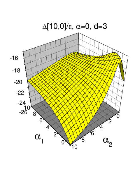
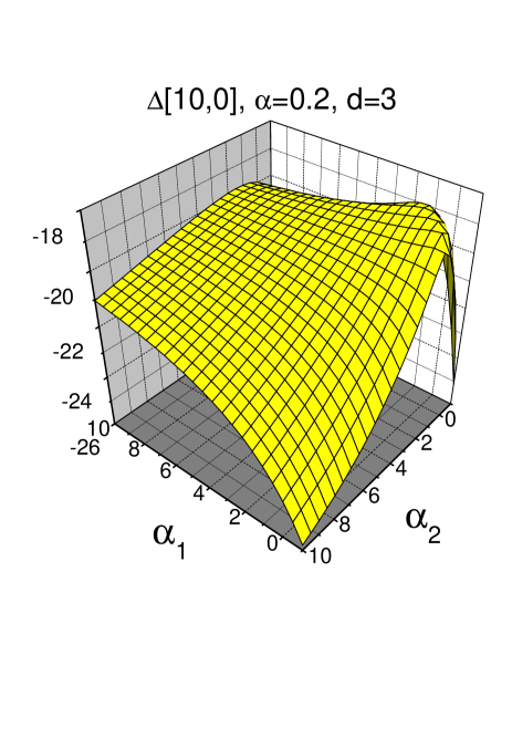
Figure 14: Behavior of the critical dimension $\Delta[10,0]/\varepsilon$ on anisotropy parameters $\alpha_{1}$ and $\alpha_{2}$ for $\alpha=0$ (incompressible case) and for $\alpha=0.2$.

The renormalization matrix $Z_{[N,p]\,[N,p^{\prime}]}$ is then found from the condition that $F^{R}[N,p]$ from Eq. (61) must be free of UV divergences when are written in renormalized variables, i.e., it does not contain poles in $\varepsilon$. In the MS scheme one obtains

$$Z_{[N,p][N,p+2(i-2)]}=\delta_{2i}+\frac{g\,S_{d}}{(2\pi)^{d}}\frac{A}{8\varepsilon}\,Q_{i}$$ (64)

where $i=1,2,3,4$, $A=1/(d^{2}\chi^{2}(d+2)(d+1))$, and coefficients $Q_{i},i=1,2,3,4$ are given in Eq. (63). In the end, from Eq. (64) and using definitions (53), one finds the following expressions for the elements of the matrix of anomalous dimensions $\gamma_{[N,p]\,[N^{\prime},p^{\prime}]}$

$$\gamma_{[N,p][N,p+2(i-2)]}=-\frac{g\,S_{d}}{(2\pi)^{d}}\frac{A}{4}\,Q_{i}$$ (65)

for $i=1,2,3,4$ and the matrix of critical dimensions (55) has the form

$$\Delta_{[N,p][N,p^{\prime}]}=N\,\varepsilon+\gamma_{[N,p][N,p^{\prime}]}^{*},$$ (66)

where the asterisk means that $\gamma_{[N,p][N,p^{\prime}]}$ is taken at the fixed point given by Eqs. (36) and (37). Eq. (66), which depends on the anisotropy parameters $\alpha_{1},\alpha_{2}$, as well as on the compressibility parameter $\alpha$, is desired one-loop expression for the matrix of critical dimensions of the composite operators (57).

5.3 Anomalous scaling: one-loop approximation

The critical dimensions of the operators $F[N,p]$, which we denote as $\Delta[N,p]$, are after all equal to the eigenvalues of the matrix of critical dimensions (66). In the isotropic case or in the case with large-scale anisotropy, where the matrix (66) is triangular, the eigenvalues are equal directly to the diagonal elements of the matrix. This fact allows us to assign uniquely the concrete critical dimension to the corresponding composite operator even in the case with small-scale anisotropy and study their hierarchical structure as a functions of $p$ (see [29] for details). In Ref. [29] it was shown that some of the critical dimensions are negative, therefore they lead to the anomalous scaling (singular behavior of the scaling functions). At the same time, the leading role is played by the operators with the most negative critical dimensions which are the operators with $p=0$ for the structure functions (44) with even $N$, and the operators with $p=1$ for the structure functions with odd $N$.

Thus, the combination of the RG representation with the OPE (49) leads to the final asymptotic expression for the structure functions (44) within the inertial range

$$S_{N}({\bf r})=D_{0}^{-N/2}r^{N(1-\varepsilon)}\sum_{N^{\prime}\leq N}\sum_{p}\{C_{N^{\prime,p}}\,(r/L)^{\Delta[N^{\prime},p]}+\dots\}\,,$$ (67)

where $p$ obtains all possible values for given $N^{\prime}$, $C_{N^{\prime,p}}$ are numerical coefficients which are functions of the parameters of the model, and dots means contributions by the operators others than $F[N,p]$ (see, e.g., [21, 29] for details).

In what follows, we shall investigate the influence of compressibility on the picture found in Ref. [29]. Our aim is to find the answer on the question whether the presence of compressibility leads to the more pronounced anomalous scaling of structure functions of the scalar field or not. Another purpose of the present analysis is to check whether the combine effects defined by compressibility and small-scale anisotropy can lead to the more complicated structure of critical dimensions than it was studied in Ref. [29] (see also Ref. [HnHoJuMaSp05]). One possibility is that the pairs of complex conjugate eigenvalues of the matrix of critical dimensions can exist. It leads to the oscillation behavior of the corresponding scaling function [29], i.e., the scaling functions in Eq. .(67) would contain terms of the following form

$$(r/L)^{\Delta_{R}}\left\{c_{1}\cos\left[\Delta_{I}(r/L)\right]+c_{2}\sin\left[\Delta_{I}(r/L)\right]\right\},$$ (68)

where $\Delta_{R}$ and $\Delta_{I}$ are real and imaginary part of $\Delta$, and $c_{1,2}$ are constants. Another possibility is related to the situation if the matrix of critical dimensions cannot be diagonalized and has only the Jordan form. Then a logarithmic correction would be involved to the powerlike behavior (see Ref. [29]).

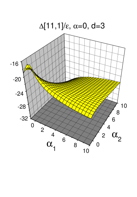
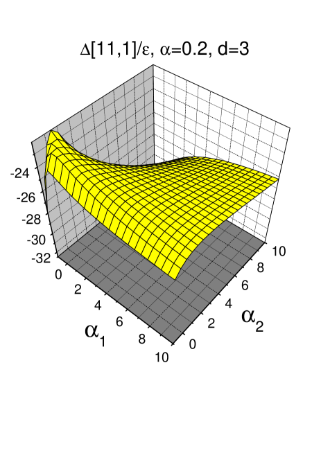
Figure 15: Behavior of the critical dimension $\Delta[11,1]/\varepsilon$ on anisotropy parameters $\alpha_{1}$ and $\alpha_{2}$ for $\alpha=0$ (incompressible case) and for $\alpha=0.2$.

Behavior of the eigenvalues of the matrix of critical dimensions $\Delta[N,p]$ for various values of $N$ for different values of the compressibility parameter $\alpha$ and as the functions of the anisotropy parameters $\alpha_{1}$ and $\alpha_{2}$ are shown in Figs. 4-15. It can be immediately seen that only real eigenvalues of the corresponding matrix exist as in the incompressible case studied in Ref. [29]. At the same time, the hierarchical structure of the critical dimensions for different values of $p$ and the same $N$ shown in Ref. [29] is also preserved. The dependence of the critical dimension $\Delta[2,0]$ is not shown because it is identically equal to zero. It can be shown either by direct calculation or by using the Schwinger equation (see, e.g., Ref. [29]). All the figures show that compressibility leads to smaller values of the critical dimensions of the corresponding composite operators, thus, at the same time, to the more noticeable anomalous scaling. As it is shown in the figures, the effects of compressibility are the most pronounced for small values of the anisotropy parameters, as well as for the negative values of these parameters. On the other hand, in the limit of large positive values of anisotropy parameters $\alpha_{1}$ and $\alpha_{2}$ the effects of compressibility tend to zero. Especially, in the limit $\alpha_{1,2}\rightarrow\infty$ the influence of compressibility is vanished completely which can be shown by direct analytical investigation.

6 Conclusion

In this paper we have analyzed asymptotic behavior of the single-time structure functions $S_{N}(r)$ of a passively advected scalar field by the compressible velocity field with small-scale anisotropy by using the field-theoretic renormalization group and the operator product expansion in a minimal-subtraction scheme of analytical renormalization.

It is shown that the leading-order powerlike asymptotic behavior of the single-time structure functions of a scalar field within the inertial range in our compressible anisotropic case is given by the critical dimensions of the same composite operators as in the incompressible anisotropic case but now they acquire rather strong dependence on the compressibility parameter. Further, it is shown that when the parameter of compressibility is increasing then the critical dimensions of relevant composite operators become smaller, therefore, within our model, we can conclude that the anomalous scaling of the structure functions of a passive scalar quantity advected by a given velocity field is more pronounced in the compressible stochastic environment than in the incompressible one (see Figs. 4-15). Concrete calculations were done up to the structure functions of order $N=11$. In our calculations we have not found possible oscillatory modulation (related to the possible existence of the complex conjugate eigenvalues of the matrix of critical dimensions), as well as we have not found possible logarithmic corrections (related to the fact that the corresponding matrix can has only Jordan form) to the leading powerlike asymptotic. Thus, all calculated corrections have had purely powerlike behavior.

It is also shown that the critical dimensions are ordered hierarchically as in the incompressible case [29], i.e., the compressibility does not disturb the anisotropic structure of the critical dimensions rather it shifts them toward smaller values. The largest shift of the critical dimensions is present for negative and small positive values of the anisotropy parameters. On the other hand, when the anisotropy parameters tend to infinity the effects of compressibility vanish.

Acknowledgments

The work was supported in part by VEGA grant 6193 of Slovak Academy of Sciences and by Science and Technology Assistance Agency under contract No. APVT-51-027904.

Appendix

The explicit form of the coefficients $A_{ij}$ and $B_{ij}$ with $i=1,2,3,4$ and $j=0,1$ (see Eq. (63)) is

$$A_{10} = p(p-1)d(1+d)((\alpha_{1}-\alpha_{2})(2+d)-(d+2+\alpha_{2}(1+d)+\alpha_{1}(d^{2}-3))\chi$$

$$+(d-2+\alpha_{2}+\alpha_{1}(1+d)+d^{2})\chi^{2})),$$

$$A_{11} = p(p-1)d(1+d)(2+d)(1+\chi)\chi,$$

$$B_{10} = p(p-1)(-(\alpha_{1}-\alpha_{2})d(1+d)(2+d)+(1+d)(2+d)(\alpha_{2}(d-1)+\alpha_{1}(d-1)^{2}+d)\chi$$

$$-(d^{2}-1)(-2+\alpha_{1}+\alpha_{2}+d+\alpha_{1}d+d^{2})\chi^{2}),$$

$$B_{11} = p(p-1)(-(1+d)(2+d)d\chi-(d+2)(d^{2}-1)\chi^{2}),$$

$$A_{20} = d(4n(n-1)(1+\chi)(3(2+d)(\chi-\alpha_{1})+\alpha_{1}(d^{2}-1)\chi$$

$$+3\alpha_{2}(2+d+\chi(1+d)))-(1+d)(p(p-1)(-d(2+d)\chi+\alpha_{1}(d(2+d)$$

$$+2\chi(1+\chi))-\alpha_{2}(1+\chi)(d(2+d(1+\chi))-2\chi))$$

$$-2((2+d)\chi(\alpha_{2}-\alpha_{1}+(\alpha_{2}+\alpha_{1}(d-1)+d)\chi)$$

$$-2(-(2+d)\chi((d-3)\chi-3)+\alpha_{2}(1+\chi)(6+3d+\chi+2d\chi)$$

$$+\alpha_{1}(d^{2}\chi+(\chi-6)(1+\chi)-d(3+\chi(2+\chi))))p)n)),$$

$$A_{21} = d(-12n(n-1)(1+\chi)(2+d)\chi+(1+d)(-p(p-1)d(2+d)\chi$$

$$+12(1+\chi)(2+d)\chi pn)),$$

$$B_{20} = -4n(n-1)(-3(\alpha_{1}-\alpha_{2})d(2+d)+(2+d)(3d-3\alpha_{2}+6\alpha_{2}d$$

$$+\alpha_{1}(3+(d-5)d))\chi+(7d-6-3\alpha_{2}+(3+3\alpha_{2}-d)d^{2}$$

$$+\alpha_{1}(d-1)^{2}(1+d))\chi^{2})+(1+d)(p(p-1)((\alpha_{1}-\alpha_{2})d^{2}(2+d)$$

$$-d(2+d)(2\alpha_{2}(-1+d)+d)\chi-(d-1)(-2(\alpha_{1}+\alpha_{2})+\alpha_{2}d^{2})\chi^{2})$$

$$-2((2+d)\chi((\alpha_{2}-\alpha_{1})d+(\alpha_{2}(d-1)+\alpha_{1}(d-1)^{2}+d)\chi)$$

$$+2(3(\alpha_{1}-\alpha_{2})d(2+d)-(2+d)(\alpha_{1}(d-3)(d-1)+3d-3\alpha_{2}+5\alpha_{2}d)\chi$$

$$+(d-1)(-6-\alpha_{1}-\alpha_{2}+(\alpha_{1}-2\alpha_{2}-1)d+d^{2})\chi^{2})p)n),$$

$$B_{21} = -12n(n-1)(-(2+d)d\chi+(2-3d-2d^{2})\chi^{2})-(1+d)(-p(p-1)d^{2}(2+d)\chi$$

$$+2(-(2+d)d\chi^{2}+6(2+d)\chi(d+(d-1)\chi)p)n),$$

$$A_{30} = -2d(2+d)(2n(n-1)(-6\alpha_{1}(2+d)+\alpha_{1}((d-5)d-12)\chi$$

$$+6\alpha_{2}(1+\chi)(2+d+\chi+d\chi)+\chi(12(1+\chi)+d(6+5\chi-d\chi)))$$

$$+(1+d)(d\chi(-\alpha_{1}+\alpha_{2}+\chi+\alpha_{2}\chi)-2(-\alpha_{1}(2+d+2\chi)+\chi(2+d+2\chi)$$

$$+\alpha_{2}(1+\chi)(2+d+d\chi))p)n),$$

$$A_{31} = 2d(2+d)(12n(n-1)(1+\chi)(2+d)\chi-(1+d)(-d\chi^{2}+2(\chi(2+d+2\chi))p)n),$$

$$B_{30} = 2(2+d)(2n(n-1)(-6(\alpha_{1}-\alpha_{2})d(2+d)+(6(2+d)(d+\alpha_{2}(2d-1))$$

$$+\alpha_{1}(12+d(-12+(d-5)d)))\chi+(-12+d(12-(d-5)d)$$

$$+\alpha_{2}(d-6+7d62))\chi^{2})+(1+d)(d\chi(-\alpha_{1}d+d\chi+\alpha_{2}(d+2(d-1)\chi))$$

$$-2(-(\alpha_{1}-\alpha_{2})d(2+d)+(-2\alpha_{1}(d-1)+d(2+d)+2\alpha_{2}(d-1+d^{2}))\chi$$

$$+(d-1)(2+\alpha_{2}d)\chi^{2})p)n),$$

$$B_{31} = 2(2+d)(12n(n-1)(-\chi(d(2+d)(1+\chi)-2\chi))$$

$$+(1+d)(-d^{2}\chi^{2}+2(\chi(d(2+d)+2(d-1)\chi))p)n),$$

$$A_{40} = 4n(n-1)d(2+d)(\alpha_{2}(4+d)(1+\chi)(2+d+\chi+d\chi)$$

$$-\alpha_{1}(8(1+\chi)+d(6+d+5\chi))+\chi(8(1+\chi)+d(6+d+5\chi))),$$

$$A_{41} = -4n(n-1)d(2+d)\chi(8(1+\chi)+d(6+d+5\chi)),$$

$$B_{40} = 4n(n-1)(2+d)((\alpha_{1}-\alpha_{2})d(2+d)(4+d)-(2+d)(\alpha_{1}(4-5d)$$

$$+(4+d)(d+\alpha_{2}(2d-1)))\chi-((2+d)(5d-4)+\alpha_{2}(-4+d^{2}(5+d)))\chi^{2}),$$

$$B_{41} = 4n(n-1)(2+d)(d(2+d)(4+d)\chi+(-8+6d+5d^{2})\chi^{2}),$$

References

- [1] R. H. Kraichnan, Phys. Fluids 11, 945 (1968).
- [2] A. S. Monin, A. M Yaglom, Statistical Fluid Mechanics (MIT Press, Cambridge, MA, 1975), Vol. 2.
- [3] Turbulence and Stochastic Processes, edited by J. C. R. Hunt, O. M. Philips, and D. Williams [Proc. R. Soc. London, Ser. A 434, 1-240 (1991)].
- [4] W. D. McComb, The Physics of Fluid Turbulence (Clarendon, Oxford, 1990).
- [5] U. Frisch, Turbulence: The Legacy of A.N. Kolmogorov (Cambridge University Press, Cambridge, 1995).
- [6] R. A. Antonia, E. J. Hopfinger, Y. Gagne, and F. Anselmet, Phys. Rev. A 30, 2704 (1984).
- [7] K. R. Sreenivasan, Proc. R. Soc. London, Ser. A 434, 165 (1991).
- [8] M. Holzer and E. D. Siggia, Phys. Fluids 6, 1820 (1994).
- [9] A. Pumir, Phys. Fluids 6, 2118 (1994).
- [10] C. Tong and Z. Warhaft, Phys. Fluids 6, 2165 (1994).
- [11] T. Elperin, N. Kleeorin, and I. Rogachevskij, Phys. Rev. E 52, 2617 (1995); Phys. Rev. Lett. 76, 224 (1996); Phys. Rev. E 53, 3431 (1996).
- [12] K. Gawedzki and A. Kupiainen, Phys. Rev. Lett. 75 (1995) 3834; D. Bernard, K. Gawedzki, and A. Kupiainen, Phys. Rev. E 54 (1996) 2564; M. Chertkov, G. Falkovich, I. Kolokov, and V. Lebedev, Phys. Rev. E 52 (1995) 4924; M. Chertkov and G. Falkovich, Phys. Rev. Lett. 76 (1996) 2706.
- [13] B. I. Shraiman and E. D. Siggia, Phys. Rev. Lett. 77, 2463 (1996); A. Pumir, B. I. Shraiman, and E. D. Siggia, Phys. Rev. E 55, R1263 (1997).
- [14] A. Pumir, Europhys. Lett. 34, 25 (1996); 37, 529 (1997); Phys. Rev. E 57, 2914 (1998).
- [15] M. Avellaneda and A. Majda, Commun. Math. Phys. 131, 381 (1990); 146, 139 (1992); A. Majda, J. Stat. Phys. 73, 515 (1993); D. Horntrop and A. Majda, J. Math. Sci. Univ. Tokyo 1, 23 (1994).
- [16] Q. Zhang and J. Glimm, Commun. Math. Phys. 146, 217 (1992).
- [17] R. H. Kraichnan, Phys. Rev. Lett. 72, 1016 (1994).
- [18] R. H. Kraichnan, V. Yakhot, and S. Chen, Phys. Rev. Lett. 75, 240 (1995).
- [19] G. Falkovich, K. Gawȩdzki, M. Vergassola, Rev. Mod. Phys. 73, 913 (2001).
- [20] J. Zinn-Justin, Quantum Field Theory and Critical Phenomena (Clarendon, Oxford, 1989).
- [21] A. N. Vasil’ev, Quantum-Field Renormalization Group in the Theory of Critical Phenomena and Stochastic Dynamics (St. Petersburg Institute of Nuclear Physics, St. Petersburg, 1998) [in Russian; English translation: Gordon & Breach, 2004].
- [22] C. de Domoinicis and P.C. Martin, Phys. Rev. A 19, 419 (1979).
- [23] L. Ts. Adzhemyan, A. N. Vasil’ev, and Yu. M. Pis’mak, Theor. Math. Phys. 57, 1131 (1983).
- [24] L. Ts. Adzhemyan, A. N. Vasil’ev, and M. Hnatich, Theor. Math. Phys. 58, 47 (1984).
- [25] L. Ts. Adzhemyan, N. V. Antonov, and A. N. Vasil’ev, Usp. Fiz. Nauk 166, 1257 (1996) [Phys. Usp. 39, 1193 (1996)].
- [26] L. Ts. Adzhemyan, N. V. Antonov, and A. N. Vasil’ev, The Field Theoretic Renormalization Group in Fully Developed Turbulence (Gordon Breach, London, 1999).
- [27] L. Ts. Adzhemyan, N. V. Antonov, and A. N. Vasil’ev, Phys. Rev. E 58, 1823 (1998); Theor. Math. Phys. 120, 1074 (1999).
- [28] L. Ts. Adzhemyan, N. V. Antonov, V. A. Barinov, Yu. S. Kabrits, and A. N. Vasil’ev, Phys. Rev. E 64, 056306 (2001); ibid. 63, 025303(R) (2001).
- [29] L. Ts. Adzhemyan, N. V. Antonov, M. Hnatich, and S. V. Novikov, Phys. Rev. E 63, 016309 (2000).
- [30] L. Ts. Adzhemyan, and N. V. Antonov, Phys. Rev. E 58, 7381 (1998).
- [31] N. V. Antonov, and J. Honkonen, Phys. Rev. E 63, 036302 (2001).
- [32] N. V. Antonov, Phys. Rev. E 60, 6691 (1999).
- [33] N. V. Antonov, Physica D 144, 370 (2000); Zap. Nauchn. Semin. POMI 269, 79 (2000).
- [34] L. Ts. Adzhemyan, N. V. Antonov and J. Honkonen, Phys. Rev. E 66, 036313 (2002); M. Hnatič, E. Jurčišinová, M. Jurčišin and M. Repašan, J. Phys. A: Math. Gen. 39, 8007 (2006); O. G. Chkhetiani, M. Hnatich, E. Jurčišinová, M. Jurčišin, A Mazzino, and M. Repašan, Czech. J. Phys. 56, 827 (2006); J. Phys. A: Math. Gen. 39, 7913 (2006); Phys. Rev. E 74, 036310 (2006).
- [35] A. Lanotte and A. Mazzino, Phys. Rev. E 60, R3483 (1999); N. V. Antonov, A. Lanotte, and A. Mazzino, ibid. 61, 6586 (2000); A. Celani, A. Lanotte, A. Mazzino, and M. Vergassola, Phys. Rev. Lett. 84, 2385 (2000).
- [36] I. Arad, L. Biferale, and I. Procaccia, Phys. Rev. E 61, 2654 (2000); I. Arad, V. L’vov, E. Podivilov, and I. Procaccia, ibid. 62, 4904 (2000).
- [37] S. Kurien, K. G. Aivalis, and K. R. Sreenivasan, J. Fluid Mech. 448, 279 (2001); M. M. Afonso and M. Sbragaglia, J. Turbulence 6, 10 (2005);
- [38] S. G. Saddoughi and S. V. Veeravalli, J. Fluid Mech. 268, 333 (1994); V. Borue and S. A. Orszag, ibid. 306, 293 (1996).
- [39] I. Arad, B. Dhruva, S. Kurien, V. S. L’vov, I. Procaccia, and K. R. Sreenivasan, Phys. Rev. Lett. 81, 5330 (1998); I. Arad, L. Biferale, I. Mazzitelli, and I. Procaccia, ibid. 82, 5040 (1999); S. Kurien, V. S. L’vov, I. Procaccia, and K. R. Sreenivasan, Phys. Rev. E 61, 407 (2000); S. Kurien and K. R. Sreenivasan, ibid. 62, 2206 (2000); I. Arad, V. S. L’vov, and I. Procaccia, Physica A 288, 280 (2000); L. Biferale and F. Toschi, Phys. Rev. Lett. 86, 4831 (2001); I. Arad and I. Procaccia, Phys. Rev. E 63, 056302 (2001); L. Biferale, I. Daumont, A. Lanotte, and F. Toschi, ibid. 66, 056306 (2002); V. S. L’vov, I. Procaccia, and V. Tiberkevich, ibid. 67, 026312 (2003); L. Biferale, G. Boffetta, A. Celani, A. Lanotte, and F. Toschi, Phys. Fluids 15, 2105 (2003).
- [40] K. Yoshida and Y. Kaneda, Phys. Rev. E 63, 016308 (2001); K. Yoshida, T. Ishihara, and Y. Kaneda, Phys. Fluids 15, 2385 (2003).
- [41] L. Biferale and I. Procaccia, Phys. Rep. 414, 43 (2005).
- [42] A. Bigazzi, L. Biferale, S. M. A. Gama, and M. Velli, Astrophys. J. 638, 499 (2006).
- [43] L. Sorriso-Valvo, V. Carbone, R. Bruno, and P. Veltri, Europhys. Lett. 75, 832 (2006).
- [44] L. D. Landau and E. M. Lifshitz, Fluid Mechanics, 2nd ed. (Pergamon Press, Oxford, 1987).
- [45] A. M. Obukhov, Izv. Akad. Nauk SSSR, Geogr. Geofiz. 13, 58 (1949).
- [46] G. Eyink, Phys. Rev. E 54, 1497 (1996); G. Eyink and J. Xin, Phys. Rev. Lett. 77, 2674 (1996).
- [47] R. H. Kraichnan, Phys. Rev. Lett. 78, 4922 (1997).
- [48] I. S. Gradshtejn and I. M. Ryzhik, Tables of Integrals, Series and Products (Academic, New York, 1965).
- [49] P. C. Martin, E. D. Siggia, H. A. Rose, Phys. Rev. A 8, 423 (1973).
- [50] J. C. Collins, Renormalization. An Introduction to Renormalization, the Renormalization Group, and the Operator Product Expansion (Cambridge University Press, Cambridge, 1984).