Via Hexagons to Squares in Ferrofluids:
Experiments on Hysteretic Surface Transformations under Variation of the Normal Magnetic Field

Abstract

We report on different surface patterns on magnetic liquids following the Rosensweig instability. We compare the bifurcation from the flat surface to a hexagonal array of spikes with the transition to squares at higher fields. From a radioscopic mapping of the surface topography we extract amplitudes and wavelengths. For the hexagon–square transition, which is complex because of coexisting domains, we tailor a set of order parameters like peak–to–peak distance, circularity, angular correlation function and pattern specific amplitudes from Fourier space. These measures enable us to quantify the smooth hysteretic transition. Voronoi diagrams indicate a pinning of the domains. Thus the smoothness of the transition is roughness on a small scale.

1 Introduction

The formation of static liquid mountains, floating on the free surface of a magnetic fluid (MF), when subjected to a vertical magnetic field is a fascinating phenomenon. It was uncovered by cowley1967 soon after the synthesis of the first ferrofluids and thus has served as a “coat of arms” for the field of magnetic fluid research. The fascination stems in part from the fact that liquid crests which persist without motion are not a familiar experience (see Figure 1 a).

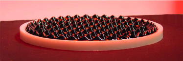
(a) (b)

Figure 1: The Rosensweig instability. Photo of the Rosensweig pattern (a) and bifurcation diagram (b) following friedrichs2001.

In contrast to pattern formation in dissipative systems [cross1993] the phenomenon can be described by an energy functional, which comprises hydrostatic, magnetic and surface energy [gailitis1969, kuznetsov1976, gailitis1977]. As the surface profile deviates from the flat reference state, the contributions of the hydrostatic and the surface energy grow whereas the magnetic energy decreases. For a sufficiently large magnetic induction $B>B_{c}$, this gives rise to the normal field, or Rosensweig, instability. By minimizing the energy functional an amplitude equation can be derived, which has three roots [friedrichs2001], describing liquid ridges, squares and hexagons, as sketched in Figure 1 (b). The hexagons appear first due to a transcritical bifurcation and their amplitude is given by

$$A_{H}=\frac{\gamma(1+\varepsilon)+\sqrt{\gamma^{2}(1+\varepsilon)^{2}+4\,\epsilon g_{\mathrm{h}}}}{2g_{\mathrm{h}}},$$ (1)

where $\varepsilon=(B^{2}-B_{c}^{2})/B_{c}^{2}$ is the bifurcation parameter, and $\gamma$, $g_{\mathrm{h}}$ are scaling parameters. The hysteretic range $[\varepsilon_{\mathrm{F}},0]$ increases with increasing susceptibility $\chi$. Moreover we have a supercritical bifurcation to squares, which become stable in the region $\varepsilon_{S}<\varepsilon<\varepsilon_{\lambda}$. Their amplitude is described by

$$A_{S}=\sqrt{\frac{\varepsilon}{g_{\mathrm{s}}}}.$$ (2)

The bifurcation to ridges is also supercritical [zaitsev1969], but they are always unstable. The parameters $g_{\mathrm{h}}$, $g_{\mathrm{s}}$, and $\gamma$ depend on the wave number $k$ and the susceptibility $\chi$ and can be estimated for rather small $\chi$ only [friedrichs2001].

The hexagon branch is subcritical, which complicates a quantitative description of the Rosensweig instability, both in the linear, as well as in the nonlinear approach.

A linear description of the Rosensweig instability is amenable in theory, but restricted to small amplitudes. In experiments however, small amplitudes are short-lived. Thus a new pulse technique has been applied in order to measure the wave number of maximal growth during the increase of the pattern [lange2000]. Also the decay of metastable patterns within the linear regime has been investigated in theory and experiment by reimann2003. Predictions for the growth rate of the pattern amplitude by lange2001 are tested by means of a novel magnetic detection technique [reimann2005], which is capable to measure the pattern amplitude with a high resolution in time (7k samples/sec). The achievementsin the linear regime are summarized by lange2006 and richter2006.

A nonlinear description of the instability is, despite the progress reported above, still restricted to small susceptibilities and a linear magnetization law. Thus a full numerical approach to the nonlinear problem, based on the finite element method (FEM), is most welcome. Its achievements are reported in this issue [lavrova2006b]. From an experimental point of view, the final, nonlinear state is difficult to access because the dark and steep structures are an obstacle for standard optical measurement techniques. Thus we developed a new approach to record the full surface profiles, from which the bifurcation diagram can than be established. The results obtained in the hexagonal regime are summarized in the next section. The further parts of the article are devoted to new investigations focusing on the transition from the hexagonal to the square planform.

2 Review of the Results in the Hexagonal Regime

To overcome the hindrances to optical observation we utilize a radioscopic technique which is capable to record the full surface relief in the centre of the vessel, far away from distortions by the edges [richter2001]. The experimental setup is sketched in figure 2 (a). A Teflon^® vessel is filled with MF up to the brim and placed on the common axis midway between a Helmholtz pair of coils. An X-ray tube is mounted above the centre of the vessel at a distance of 1606 mm. The radiation transmitted through the fluid layer and the bottom of the vessel is recorded by an X-ray sensitive photodiode array detector (16 bit). The full surface relief, as presented in figure 2 (b) is then reconstructed from the calibrated radioscopic images.

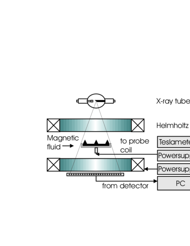
(a) (b)

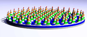
Figure 2: Measuring the surface relief via radioscopy: (a) principle of the experimental setup, (b) reconstructed surface relief. The radius of the vessel is $60\,$mm, its depth $3\,$mm. The colour stripes have a width of $1\,$mm. The parameters of the fluid EMG 901 (Ferrotec) are: $\chi=2.2$, $\rho=1.406\rm\,g\,cm^{-3}$, and $\sigma=25\pm 0.7\rm\,mN/m$. Figures from richter2005

With this set-up we measured the top-to-bottom amplitude $A$ of the fluid pattern in the centre of the vessel. Figure 3 (a) displays the hysteretic behavior of $A(B)$ for the adiabatic increase and decrease of $B$, depicted by crosses and dots, respectively. The solid and dashed lines display a convincing fit to (1). We used a concentrated MF ($\chi=2.2$) to realize a large hysteretic regime, enabling us to investigate the stability of the flat surface against local perturbations, within the bistable regime. For that purpose a small cylindrical air coil was placed under the centre of the vessel, as depicted in figure 2 (a). This allows for a local increase of the magnetic induction. A local pulse of $B_{+}=0.68\,\mbox{\rm mT}$ added to the uniform field of $B=8.91\,\rm mT$ produces a single stationary spike of fluid, surrounded by a circular dip, which does not disperse after $B_{+}$ has been turned off. The inset of figure 3 (a) gives a picture of this radially-symmetric state which will be referred to as a ferrosoliton. The range of stability of a soliton is marked in figure 3 (a) by full squares and full circles alongside the hysteretic regime.

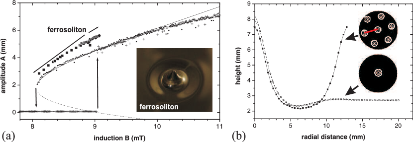
Figure 3: (a) The amplitude of the pattern versus the magnetic induction. The crosses (dots) mark the values for increasing (decreasing) induction, respectively. The solid (dashed) lines display the least squares fit to (1) with $\gamma=0.281$ and $g_{\mathrm{h}}=0.062$. The full circles (squares) give the amplitude of the localized spike (see inset) initiated at $B=8.91\,\rm mT$ for increasing (decreasing) induction respectively. (b) Height profiles for one period of the hexagonal pattern (filled squares), and for two different solitons (marked by open symbols and a dashed line). Figures from richter2005

The ferrosoliton is a stable non-decaying structure; it remains intact for days – for a movie see castelvecchi2005. In contrast to previously detected dissipative 2d-solitons, like oscillons [umbanhowar1996], it is a static object without any dissipation of energy. Thus the stabilization mechanism discussed for dissipative 2d-solitons, a balance of dissipation versus nonlinearity, can not be valid here. In order to shed some light on its stabilization mechanism we compare in figure 3 (b) the height profile of solitons with the one of regular Rosensweig peaks. The width of the soliton is equal to the period of the lattice. This indicates that a spreading of the local perturbation is locked by the periodicity of the Rosensweig lattice, as suggested in a general context by pomeau1986. This wave-front locking could be verified in a conservative analogue of the Swift–Hohenberg equation [richter2005].

Figure 4: Comparison of experimental and numerical results. (a) The pattern amplitude for increasing (decreasing) $\varepsilon$ is denoted by upward (downward) triangles, respectively. (b) The peak profiles at $\varepsilon=0.35$ for increasing (decreasing) $\varepsilon$ are marked by squares (circles), respectively. The solid lines give the corresponding numerical results. Figures from gollwitzer2006.

From qualitatively new features we turn our attention now to a quantitative comparison of experimental and numerical results. To make the comparison more feasible, we used a deeper container ($h=10\,$mm). Its floor is flat within a diameter of $130\,$mm, outside of which it is inclined upwards at $32$ degrees, so that the thickness of the fluid layer smoothly decreases down to zero towards the side of the vessel. We select a MF available in large amounts, which has a smaller susceptibility ($\chi=1.17$). Figure 4 (a) displays the evolution of the pattern amplitude (triangles), which shows a reduced hysteresis in comparison to figure 3 due to the reduced $\chi$. The two solid lines give the result of the FEM calculations taking into account the measured fluid parameters and the nonlinear magnetization curve, as presented in detail by gollwitzer2006. Note, that the agreement was obtained without any free fitting parameter. Figure 4 (b) displays the measured and calculated peak profiles, which match as well.

3 The Hexagon–Square-Transition

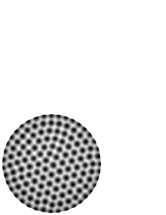
(a) (b) (c) (d)

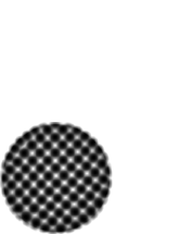
Figure 5: X-ray absorption images of two different states of the pattern observed with the fluid APG 512 A from Ferrotec. Fluid parameters are: initial susceptibility $\chi=1.17$, density $\rho=1236\,\mathrm{kg\,m^{-3}}$, surface tension $\sigma=30.6\,\mathrm{mN\,m^{-1}}$, viscosity $\eta=120\,\mathrm{mPa\,s}$. Hexagonal pattern (a) observed at $B=19.78\,\mathrm{mT}$ and square pattern (d) at $B=38.05\,\mathrm{mT}$ as well as mixed states at (b) $B=21.92\,\mathrm{mT}$ and (c) $B=22.07\,\mathrm{mT}$.

Under further increase of the magnetic induction we observe a transition from the hexagonal pattern, shown in figure 5 (a) to a square one, as displayed in figure 5 (d). This transition has been previously observed by allais1985 and abou2001. The latter have investigated the role of penta–hepta defects for the mechanism of the transition. Moreover, the evolution of the wavenumber was measured for an adiabatic increase and a sudden jump of the magnetic induction. However, this remarkable studies were limited to the planform of the patterns and could not take into account the surface topography of the problem. Square patterns in MF have also been obtained in numerical investigations by boudouvis1987.

The transition between hexagonal and square planforms has been observed in other experiments, like in Bénard–Marangoni convection [thiele1998], in nonlinear optics [aumann2001] and in vibrated granular matter [melo1995]. In theory the competition between hexagons and squares has been studied for convection [malomed1990, bestehorn1996, bragard1998, herrero1994].

The transition is especially interesting, because it is a smooth morphological one. kubstrup1996, e.g., have studied fronts between hexagons and squares in a generalized Swift–Hohenberg model. They found pinning effects in domain walls separating different symmetries, as suggested by pomeau1986. These pinning effects are responsible for the static coexistence of both patterns in an extended parameter range. Note that we have observed wave-front pinning in the last paragraph as well within the context of ferrosolitons. In the different context of ferromagnetism, pinning effects between different domains of magnetic ordering are known to cause hysteresis of the order parameter [stoner1953, jiles1984]. What would be an appropriate order parameter for our context, which is capable to unveil hysteresis?

First we test the local amplitude of the central peak and the wavenumber of the pattern. Next we focuse on different order parameters tailored to this problem and adapted from various scientific fields.

3.1 Amplitude of the pattern in real space

Figure 6: Amplitude of the nonlinear pattern in real space, extracted from one single peak in the center of the dish. The triangles denote the amplitude for increasing induction, the circles for decreasing induction. The solid line is a fit with (1). The dashed line is a fit of the upper branch for $\varepsilon>1.9$ with (2). For the arrow see the body text.

We recorded 500 images at different magnetic fields, raising the induction adiabatically from $0$ to $38.1\,\mathrm{mT}$ and decreasing to zero afterwards. Figure 6 shows the dependence of the height of one single peak selected from the centre of the dish, and tracked thereafter, as a function of the applied magnetic field.

At a first glance, the amplitude seems to be continuous in spite of the picture predicted by gailitis1977 and friedrichs2001. Obviously the height of the peak is only slightly influenced by the geometry of the embedding pattern. A more careful comparison with the fit by the amplitude equation (1) of the peak heights for decreasing $\varepsilon$, however, reveals some deviations (see e.g. the arrow in figure 6). In the range above the arrow the peak is situated inside a square domain and the amplitude can therefore be fitted by (2). Below it is embedded in a hexagonal domain and hence, the fit by (1) is a convincing description of the data. Because the shift of the amplitude is small, the latter is not a sensitive order parameter for this transition.

3.2 Wavenumber of the pattern

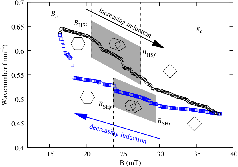
Figure 7: Wavenumber of the pattern as a function of the applied magnetic induction. Circles (squares) denote the values for increasing (decreasing) induction. In the region shaded in grey we find coexistence of hexagonal and square patterns. The horizontal line displays the capillary wavenumber $k_{c}=\sqrt{\frac{\rho g}{\sigma}}=0.63\,\mathrm{mm^{-1}}$ for comparison.

Another important measure, which discriminates between the two patterns is the wavenumber. As shown by friedrichs2001, the preferred wavenumber of squares is always less than those of hexagons in the region of coexistence. Figure 7 shows the wavenumber modulus as a function of the applied magnetic induction determined from Fourier space. We find a strong hysteresis, that goes alongside the different patterns.

When increasing the magnetic induction, the surface remains flat up to the critical induction $B_{c}=16.7\,\mathrm{mT}$, where a hexgonal array of peaks appears. Local quadratic ordering appears initially at a threshold of $B_{\mathrm{HS}i}=20.7\,\mathrm{mT}$, and the whole container is finally covered with a square pattern at $B_{\mathrm{HS}f}=27.4\,\mathrm{mT}$. Increasing the induction further, no new transition occurs until the maximum induction $B=38.1\,\mathrm{mT}$ is reached. When decreasing the field, the first hexagons appear already at $B_{\mathrm{SH}i}=29.5\,\mathrm{mT}$. Surprisingly, the comeback of the hexagons occurs at a higher field than the transition therefrom, i.e. $B_{\mathrm{SH}i}>B_{\mathrm{HS}f}$. The same holds true for the pure hexagonal pattern, which comes back at $B_{\mathrm{SH}f}=23.7\,\mathrm{mT}$, i.e. $B_{\mathrm{SH}f}>B_{\mathrm{HS}i}$. We will refer to this phenomenon as an inverse hysteresis, i.e. a proteresis [girard1989]. This observation is in agreement with abou2001. The transition can therefore not be explained by simple bistability. The wavenumber is continuous during the transition, but it has a dramatic increase between $B_{\mathrm{SH}f}$  and $B_{c}$ when decreasing the field, where it quickly relaxes to the initial value. The general tendency, that the wavenumber decreases with increasing field agrees with theoretical predictions by friedrichs2001, whereas the hysteresis effect has not been predicted.

Neither the amplitude nor the wavenumber can clearly distinguish between square and hexagonal patterns. The amplitude is provided only on the basis of local information and is therefore only slightly influenced by the geometry of the pattern. The wavenumber comprises global information and depends strongly on the pattern, but from its magnitude alone it is not possible to decide about the actual geometry. In conjunction with the distance between two adjacent peaks, however, this is possible as shown below.

3.3 Analysing the peak–to–peak distance

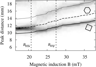
(a) (b)

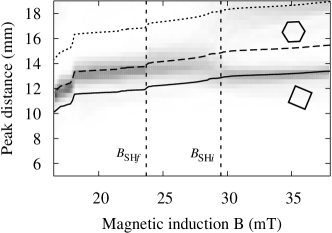
Figure 8: Histogram of the peak–to–peak distance for increasing (a) and decreasing induction (b). A high count is represented by a dark shade of gray. The lines display the theoretical distance for regular hexagons (dashed), squares (solid), and the next-to-nearest neighbours of squares (dotted) derived from the measured wavenumber.

The relation between the wavelength and the peak–to–peak distance of nearest neighbours is different for hexagons and squares: The peaks on the hexagonal grid are wider spaced by a factor of $\sqrt{3/2}$. We therefore plot a histogram of the peak–to–peak distance in figure 8 versus $B$. Thus we can compare the distance distribution to the wavelength, which is plotted on top.

In spite of the visual observation of the transition (marked by the dashed vertical lines in figure 8 a), the peak–to–peak distance makes a rather sudden jump from the hexagonal to the square state, when the induction goes up. When decreasing the field (figure 8 b), the distribution of the peak–to–peak distances broadens in the region of coexistence.

In contrast to the plane, averaged wavelength, its combination with the peak–to–peak distance is able to discriminate between trigonal and square symmetry. This is due to a combination of information from real space and Fourier space. We will now apply this promising concept to the amplitude and its Fourier domain analogon.

3.4 Fourier-domain based correlation

(a) (b) (c)

Figure 9: Fourier transform of the pattern at three different magnetic inductions with increasing induction. (a) $B=19.78\,\mathrm{mT}$ (b) $B=22.07\,\mathrm{mT}$ (c) $B=28.92\,\mathrm{mT}$

The symmetry of the pattern is reflected in the Fourier space, as shown in figure 9. Both the hexagonal and square pattern produce clear individual peaks (a,c), while the transform of a mixture of both patterns results in a ring (b). With an angular correlation function, following millan1996, it is possible to discriminate between the amplitude contribution of each pattern: Let $\mathcal{F}(k_{x},k_{y})$ be the discrete Fourier transform of the surface relief of the pattern

$$\mathcal{F}(k_{x},k_{y})=\sum_{x=0}^{m-1}\sum_{y=0}^{n-1}h(x,y)\exp\left(-2\pi i(k_{x}x/m+k_{y}y/n)\right)$$ (3)

where $h(x,y)$ is the height of the fluid surface at the point $(x,y)$ and $m,n$ are the number of pixels in $x$ and $y$ direction, respectively. Then $\mathcal{A}=\left|\mathcal{F}(k_{x},k_{y})\right|$ denotes the corresponding amplitude. To suppress artifacts of the Fourier transform coming from the boundary, we apply a cylindrically symmetric Hamming window of the width $b$ with the weight function

$$w(x,y)=\cases{\left(0.54+0.46\cos\left(\frac{\pi\sqrt{x^{2}+y^{2}}}{b}\right)\right)^{2}&for $x^{2}+y^{2}\leq b^{2}$\\ 0&else.}$$ (4)

Then we define the Fourier angular correlation $P_{\alpha}$ to be

$$P_{\alpha}=\sum_{\bi{k}}\mathcal{A}(\bi{k})\mathcal{A}(R_{\alpha}\bi{k}),$$ (5)

where $R_{\alpha}$ is the matrix for rotation by the angle $\alpha$. Technically, the rotation by an arbitrary angle is done using paeth1986 algorithm.

Figure 10: Angular correlation of the pattern as a function of the angle. Solid line: Pure hexagonal pattern with a grain boundary at $B=17.5\,\mathrm{mT}$. Dashed line: Pure square pattern at $B=38.1\,\mathrm{mT}$.

This correlation function is displayed in figure 10 for two different patterns. For a perfect hexagonal lattice the Fourier transform consists of a series of delta peaks, that is invariant under a rotation by $60$ degrees. Consequently, the above defined correlation function would be zero for any angle $\alpha$ that is not an integer multiple of $60$ degrees. The same argument applies to a perfect square lattice that is invariant under a rotation by $90$ degrees. Therefore the hexagonal pattern at $B=17.5\,\mathrm{mT}$ manifests itself in major peaks at $60$ and $120$ degrees, while the square pattern at $B=38.1\,\mathrm{mT}$ yields a strong peak at $90$ degrees. Further, the correlation function will be proportional to the square of the amplitude of the corresponding lattice. Using the above defined window function (4), the amplitudes $A_{6},A_{4}$ of a square and hexagonal sinusoidal lattice in real spacen relate to the Fourier angular correlation function like

$$A_{6}=4.5\sqrt{\frac{P_{60^{\circ}}}{1.5\,mn\xi}}\quad\mbox{and}\quad A_{4}=4\sqrt{\frac{P_{90^{\circ}}}{{mn\xi}}}.$$ (6)

Here

$$\xi=\int w^{2}(x,y)\mathrm{d}x\mathrm{d}y=0.1032300545\,\pi b^{2}$$ (7)

is a normalization factor for the window function.

(a) (b)

Figure 11: Amplitude of the central peak $A$ (solid) and Fourier domain correlation amplitudes $A_{4}$ (dotted) and $A_{6}$ (dashed) of the pattern for increasing (a) and decreasing (b) magnetic induction.

Figure 11 shows the amplitude $A$ in real space, as discussed in section 3.1, together with $A_{6}$ and $A_{4}$. The amplitude of the single peak in the centre is cum grano salis an upper bound of $A_{6}$ and $A_{4}$. However, the smaller of both has an unnegligible value even for ranges, where the pattern appears to be homogeneous to the naked eye. For example, the hexagonal range $[B_{c},B_{\mathrm{HS}i}]$ in figure 11 (a) gives still a finite $A_{4}$. This is due to two differently oriented hexagonal patterns, which are tilted by an angle of 30 degrees. They are separated by a grain-boundary made of penta–hepta defects (see figure 5 a). The tilted smaller patch manifests itself as the intermediate structure between the major peaks in Fourier space in figure 9 (a). This leads to a positive intercorrelation between those two patterns in Fourier space at 90 degrees.

When increasing the field, this grain boundary moves to the border immediately before $B=B_{\mathrm{HS}i}$ and therefore $A_{4}$ goes down. Right after this the transition to squares at $B=B_{\mathrm{HS}i}$ leads to an increase of $A_{4}$, which continues to follow the amplitude of the central peak, while $A_{6}$ goes down, indicating that the hexagonal pattern vanishes. However, even though at $B=B_{\mathrm{HS}f}$ the whole dish is apparently covered with squares, $A_{6}$ does not decay to zero. This is due to the noisefloor, that always leads to a finite correlation in any direction, as illustrated by the dashed line in figure 10.

The character of the transition between trigonal and square symmetry is a smooth one, which becomes clear from figure 11 (b). Both order parameters $A_{4}$ and $A_{6}$ are continuous at the transition point $B_{\mathrm{HS}i}$. This is an effect of smoothing due to the stepwise transformation of small blocks. Likewise the magnetization curve of a ferromagnet appears to be smooth, although the individual domains change their magnetization discontinuously.

In the next section we take a closer look at the mechanism for the smooth transition. For that purpose we inspect Voronoi diagrams.

3.5 Voronoi diagram for local information in real space

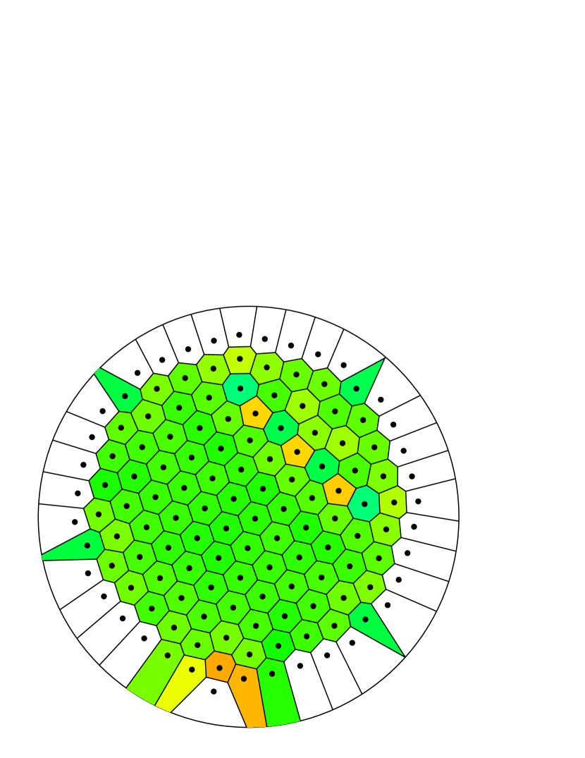
(a)

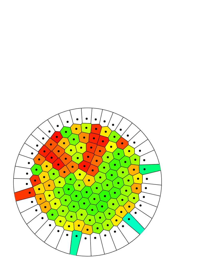
(b)

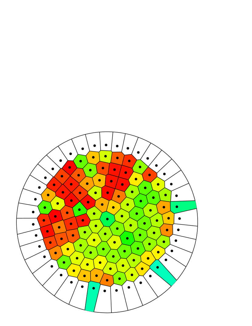
(c)

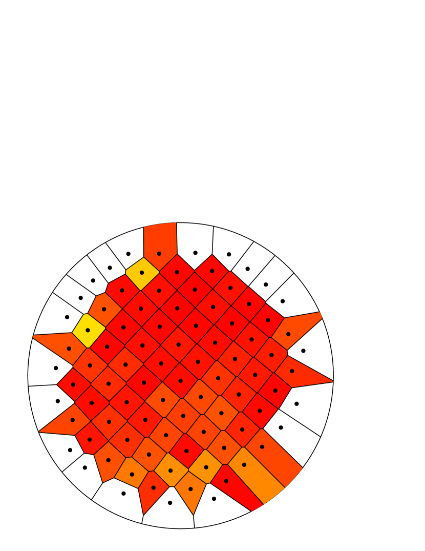
(d)

Figure 12: Coloured Voronoi diagram over the centre of the peaks for (a) $B=19.78\,\mathrm{mT}$, (b) $B=21.92\,\mathrm{mT}$, (c) $B=22.07\,\mathrm{mT}$, and (d) $B=38.05\,\mathrm{mT}$. The bar below indicates the colour code, which is derived from the maximum central angle $\alpha$ of each cell of the pattern. The colour code hue value in the HSB colour space is set to $h=1-{\nicefrac{{2\alpha}}{{\pi}}}$ with full brightness and saturation.

A classical tool for the analysis of nearest neighbours of a set of points, called sites, is the Voronoi diagram [fortune1995]. Four Voronoi diagrams for increasing magnetic induction are shown in figure 12. The two-dimensional Voronoi tesselation over a discrete set of sites

$$S=\left\{\bi{x_{i}}\right\},\bi{x_{i}}\in\mathbb{R}^{2}$$

is defined in terms of nearest neighbours: the Voronoi cell $V{x_{i}}$ corresponding to the site $\bi{x_{i}}$ is the set of points, that is closer to $\bi{x_{i}}$ than to any other site:

$$V_{\bi{x}_{i}}=\left\{\bi{x}\in\mathbb{R}^{2},\quad\left|\bi{x}-\bi{x}_{i}\right|<\left|\bi{x}-\bi{x}_{j}\right|\quad\forall j,\,j\neq i\right\}$$ (8)

The Voronoi cells are the interior of convex polygons which tesselate the entire space $\mathbb{R}^{2}$. The nearest neighbouring sites of any given site $\bi{x_{i}}$ are then defined by all $\bi{x_{j}}$, where the Voronoi cell $V{x_{j}}$ shares a common edge with $V{x_{i}}$. Note that these “nearest neighbours” don’t have the same distance from $\bi{x_{i}}$ in general. This is only true for perfectly regular lattices.

We extract the position of the peaks with subpixel accuracy by fitting a paraboloid to the centre of each peak. From these coordinates we construct the Voronoi diagram. Since the Voronoi diagram of a regular hexagonal or square lattice is a regular hexagonal or square tesselation, where the sites are the centre of the cells, one might expect that the number of edges serves as a criterion of the local ordering. Unfortunately, a real quadrilateral is singular in the Voronoi diagram. An infinitesimal slight distortion of a square lattice of sites results in mostly hexagonal Voronoi cells with two tiny edges, that look like squares. But there is a number of metric quantities listed by thiele1998, namely angle, cell perimeter and cell area, which are not affected and can therefore be employed. The diagrams in figure 12 are colour coded with the maximum central angle of each cell.

This method can visualize the mechanism for the smooth transition. In figure 12 (a) almost all Voronoi cells are hexagonal (green), apart from a line of penta–hepta defects (dark green and yellow). Upon increase of $B$, this pattern remains stable up to $B_{\mathrm{HS}i}$. For $B$ slightly above $B_{\mathrm{HS}i}$, two domains of square cells have been formed (figure 12 b). The invasion of the hexagonal pattern by the square one takes place domainwise. This is corroborated when looking at (c), where another patch of squares has emerged. Obviously the domain-like transformation of the pattern is responsible for the overall smooth transition. A sudden transform into a pure square array is probably hindered by pinning of the domainfronts. The final square state is shown in figure  12 (d).

In the next section, we employ the remaining metric parameters for quantitative analysis.

3.6 Cell perimeter and area

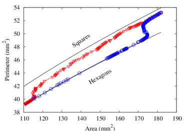
(a) (b)

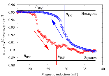
Figure 13: Hysteretic transition from hexagons to squares is shown (a) in the perimeter–area space, and (b) in the plot of the circularity $\kappa$ versus the magnetic induction. Triangles (circles) denote increasing (decreasing) magnetic induction.

According to thiele1998, the perimeter–area-ratio can be utilized to distinguish between hexagonal and square symmetry. The relations of the perimeter $\Pi$ and the area $a$ of regular planforms differ for hexagons and squares; as a function of the wavelength $\lambda$ they fulfill the following equations:

$$\Pi_{6}=4\lambda,\quad\Pi_{4}=4\lambda,\quad a_{6}=\frac{2}{3}\sqrt{3}\lambda^{2},\quad\mbox{and}\quad a_{4}=\lambda^{2}$$ (9)

Thus, a plot of the average perimeter versus the average cell area leads to a square root with different factors:

$$\Pi_{6}(a_{6})=4\sqrt{\frac{\sqrt{3}}{2}}\sqrt{a_{6}}\quad\mbox{{and}}\quad\Pi_{4}(a_{4})=4\sqrt{a_{4}}$$ (10)

Figure 13 (a) shows this plot for the experimental data, which approach the theoretical relations for regular patterns in a hysteretic manner. However, in this diagram the dependence on the control parameter $B$ is lost. We therefore define the circularity $\kappa$, a normalized area–perimeter ratio, by

$$\kappa:=\frac{\sqrt{\left<a\right>}}{\left<\Pi\right>}\cdot 2\sqrt{\pi},$$ (11)

which becomes $1$ for a perfect circle and is less for polygons. It is shown in figure 13 (b) as a function of the magnetic induction. A regular tesselation for hexagons results in $\kappa_{6}=\sqrt{\frac{\pi}{6}\sqrt{3}}\approx 0.952$ and $\kappa_{4}=\frac{\sqrt{\pi}}{2}\approx 0.886$, respectively.

This order parameter clearly shows that the hexagonal ordering is nearly perfect, because the experimental data meet the theoretical limit $\kappa_{6}$ quite well. For increasing $B$, $\kappa$ decays on a jerky path, indicating a blockwise transformation from trigonal to square symmetry – a macroscopic analogon to the Barkhausen effect. Obviously, the minimal value $\kappa_{4}$ is not reached, probably due to the instability of squares in the Voronoi tesselation. Under decrease of $B$, $\kappa$ follows a different, smoother path. All in all, the circularity shows a broad proteresis, which behaves inverse to the common hysteresis in that way, that it shows no retardation, but an advanced behaviour.

The visualization in section 3.5 uses the maximum central angle of the cells. Now we want to propose a method that makes use of all central angles of the Voronoi cells.

3.7 Angular correlation function

(a) (b)

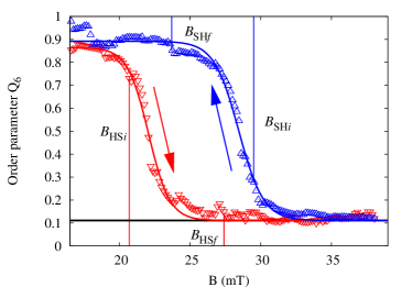
Figure 14: Angular correlation functions $Q_{4}$ (a) and $Q_{6}$ (b) in real space. The solid line in (b) marks a fit with the logistic function.

Inspired by steinhardt1983, who introduce a local order parameter in three dimensions, we propose the local angular correlation $Q_{m}$ as a transformation of the central angles:

$$Q_{m}=\left|\frac{1}{N}\sum_{i=1}^{N}e^{im\phi_{i}}\right|^{2}$$ (12)

where $\phi_{i}$ is the angle enclosed by an arbitrarily chosen axis and the line through the selected peak and its $i$-th nearest neighbour. For regular polygons with $N$ sides, this parameter gives $1$ exactly when $m$ is an integer divisor of $N$ and $0$ otherwise. For irregular polygons, the result may be any value in the range $\left[0\ldots 1\right]$. We apply the parameters $Q_{4}$ and $Q_{6}$ to our experimental data and average over all cells. Figure 14 (a) shows the hysteretic behaviour of $Q_{4}$. Though it is a normalized measure, it approaches by no means $1$. A possible explanation is that a large number of the squares are indeed degenerated hexagons, i.e. two corners are cut off at $45^{\circ}$. If all squares would be degenerated in that way, the maximum would be $Q_{4}=\frac{1}{9}$, represented by the solid horizontal line.

The complementary measure $Q_{6}$, as shown in figure 14 (b), does not suffer from these problems. It shows a smooth, nearly ideal hysteretic cycle, which can be fitted by two logistic functions. Most importantly, $Q_{6}$ clearly reflects the visual impression of the pattern, as revealed by comparison with the thresholds.

4 Summary and Conclusion

The topic of this article is twofold. First, we reported on measurements of the hexagonal surface topography, evolving after the flat surface becomes unstable due to a transcritical bifurcation. By means of radioscopy we have access to the surface reliefs. The scaling of the amplitudes obtained therefrom is in agreement with the equations deduced by friedrichs2001. Moreover, comparing the amplitudes and peak profiles from the measurements with the results obtained by matthies2005 via FEM numerics matches without further fitting parameters. Eventually, we can generate static localized states (ferrosolitons) in the bistable regime, where hexagons coexist with the flat reference state, by perturbing the surface locally.

The second part is devoted to new experimental results regarding the hexagon–square transition. Its characterization is difficult, because trigonal and quadrilateral symmetry coexist in an extended parameter range. From the recorded surface reliefs we have extracted a set of order parameters. The classical measurands, namely the amplitude and the wavenumber, show a hysteretic behaviour, but are not specific enough to catch the geometry. The combination of methods from the real and inverse space, like the peak–to–peak distance and the Fourier domain based correlation, uncovers a smooth transition between both patterns. The Voronoi diagrams reveal a domainwise transformation, suggesting a pinning mechanism. We have tailored two further measures, namely the circularity $\kappa$ and the angular correlation $Q$, which can map the complex transition in agreement with the visual impression. These show an inverse (advanced) hysteresis, called proteresis in pharmacodynamics [girard1989]. These measures may be applied to numerical calculations as well as to other experiments, providing a basis for comparison.

Both hysteretic transitions originate from the bistability of two patterns. In the first case, the energy barrier between the flat state and the hexagons is huge. Only by applying a local perturbation we can observe both states side by side in one container. The ferrosolitons are hindered to penetrate into the flat surface by pinning of the wavefronts. In the second case, the energy barrier between hexagonal and square structures appears to be lower. The pinning of the domainfronts can be overcome under variation of the control parameter, which results in a blockwise transformation. By applying noise, we expect that the first transition could be smoothed out in a similiar manner.

References

References

- [1] \harvarditemAbou et al.2001abou2001 Abou B, Wesfreid J E \harvardand Roux S 2001 416, 217–237.
- [2] \harvarditemAllais \harvardand Wesfreid1985allais1985 Allais D \harvardand Wesfreid J E 1985 Bull. Soc. Fr. Phys. Suppl. 57, 20.
- [3] \harvarditemAumann et al.2001aumann2001 Aumann A, Ackemann T, Westhoff E \harvardand Lange W 2001 Int. J. Bif. Chaos .
- [4] \harvarditemBestehorn1996bestehorn1996 Bestehorn M 1996 Phys. Rev. Lett. 76, 46–49.
- [5] \harvarditemBoudouvis et al.1987boudouvis1987 Boudouvis A G, Puchalla J L, Scriven L E \harvardand Rosensweig R E 1987 65, 307–310.
- [6] \harvarditemBragard \harvardand Velarde1998bragard1998 Bragard J \harvardand Velarde M G 1998 JFM 368, 165–194.
-
[7]
\harvarditemCastellvecchi2005castelvecchi2005
Castellvecchi D 2005 Physical Review Focus .
\harvardurlhttp://focus.aps.org/story/v15/st18 - [8] \harvarditemCowley \harvardand Rosensweig1967cowley1967 Cowley M D \harvardand Rosensweig R E 1967 30, 671.
- [9] \harvarditemCross \harvardand Hohenberg1993cross1993 Cross M C \harvardand Hohenberg P C 1993 Rev. Mod. Phys. 65(3), 851–1112.
-
[10]
\harvarditemFortune1995fortune1995
Fortune S J 1995 in D.-Z Du \harvardand F Hwang, eds, ‘Computing in
Euclidean Geometry’ Vol. 1 of Lecture Notes Series on Computing World
Scientific.
\harvardurlhttp://citeseer.ist.psu.edu/article/fortune95voronoi.html - [11] \harvarditemFriedrichs \harvardand Engel2001friedrichs2001 Friedrichs R \harvardand Engel A 2001 Phys. Rev. E 64, 021406–1–10.
- [12] \harvarditemGailitis1969gailitis1969 Gailitis A 1969 Magnetohydrodynamics 5, 44–45.
- [13] \harvarditemGailitis1977gailitis1977 Gailitis A 1977 J. Fluid Mech. 82(3), 401–413.
- [14] \harvarditemGirard \harvardand Boissel1989girard1989 Girard P \harvardand Boissel J P 1989 Journal of Pharmacokinetics and Pharmacodynamics 17(3), 401–402.
- [15] \harvarditemGollwitzer et al.2006gollwitzer2006 Gollwitzer C, Matthies G, Richter R, Rehberg I \harvardand Tobiska L 2006 submitted to J. Fluid Mech. .
- [16] \harvarditemHerrero et al.1994herrero1994 Herrero H, Perez-Garzia C \harvardand Bestehorn M 1994 Chaos 4, 15.
- [17] \harvarditemJiles \harvardand Atherton1984jiles1984 Jiles D C \harvardand Atherton D L 1984 Journal of Applied Physics 55, 2115–2120.
- [18] \harvarditemKubstrup et al.1996kubstrup1996 Kubstrup C, Herrero H \harvardand Perez-Garcia C 1996 Phys. Rev. E 54, 1560.
- [19] \harvarditemKuznetsov \harvardand Spektor1976kuznetsov1976 Kuznetsov E A \harvardand Spektor M D 1976 Sov. Phys. JETP 44, 136–141.
- [20] \harvarditemLange et al.2000lange2000 Lange A, Reimann B \harvardand Richter R 2000 Phys. Rev. E 61(5), 5528–5539.
- [21] \harvarditemLange et al.2001lange2001 Lange A, Reimann B \harvardand Richter R 2001 Phys. Rev. E 37(5), 261.
- [22] \harvarditemLange et al.2006lange2006 Lange A, Richter R \harvardand Tobiska L 2006 ‘Linear and nonlinear approach to the Rosensweig instability’ submitted to GAMM-Mitteilungen.
- [23] \harvarditemLavrova et al.2006lavrova2006b Lavrova O, Mathis G \harvardand Tobiska L 2006 Journal of Condensed Matter C xxx, xx.
- [24] \harvarditemMalomed et al.1990malomed1990 Malomed B A, Nepomnyashchy A A \harvardand Tribelsky M I 1990 Phys. Rev. A 42, 7244–7263.
- [25] \harvarditemMatthies \harvardand Tobiska2005matthies2005 Matthies G \harvardand Tobiska L 2005 J. Magn. Magn. Mater. 289, 346–349.
- [26] \harvarditemMelo et al.1995melo1995 Melo F, Umbanhowar P B \harvardand Swinney H L 1995 Phys. Rev. Lett. 75, 3838.
- [27] \harvarditemMillán \harvardand Escofet1996millan1996 Millán M S \harvardand Escofet J 1996 Applied Optics 35, 6253–6260.
- [28] \harvarditemPaeth1986paeth1986 Paeth A W 1986 in ‘Proceedings on Graphics Interface ’86/Vision Interface ’86’ Canadian Information Processing Society Toronto, Ont., Canada, Canada pp. 77–81.
- [29] \harvarditemPomeau1986pomeau1986 Pomeau Y 1986 Physica D 23, 3–11.
- [30] \harvarditemReimann et al.2005reimann2005 Reimann B, Richter R, Knieling H \harvardand Rehberg I 2005 Phys. Rev. E 71, 055202(R).
- [31] \harvarditemReimann et al.2003reimann2003 Reimann B, Richter R, Rehberg I \harvardand Lange A 2003 Phys. Rev. E 68, 036220.
- [32] \harvarditemRichter \harvardand Barashenkov2005richter2005 Richter R \harvardand Barashenkov I 2005 Phys. Rev. Lett. 94, 184503.
- [33] \harvarditemRichter \harvardand Bläsing2001richter2001 Richter R \harvardand Bläsing J 2001 Rev. Sci. Instrum. 72, 1729–1733.
- [34] \harvarditemRichter \harvardand Lange2006richter2006 Richter R \harvardand Lange A 2006 Lecture Notes in physics Springer.
- [35] \harvarditemSteinhardt et al.1983steinhardt1983 Steinhardt P J, Nelson D R \harvardand Ronchetti M 1983 Phys. Rev. B 28, 784–805.
- [36] \harvarditemStoner1953stoner1953 Stoner E C 1953 Rev. Mod. Phys. 52(1), 2–16.
- [37] \harvarditemThiele \harvardand Eckert1998thiele1998 Thiele U \harvardand Eckert K 1998 Phys. Rev. E 58(3), 3458.
- [38] \harvarditemUmbanhowar et al.1996umbanhowar1996 Umbanhowar P B, Melo F \harvardand Swinney H L 1996 Nature (London) 382, 793.
- [39] \harvarditemZaitsev \harvardand Shliomis1969zaitsev1969 Zaitsev V M \harvardand Shliomis M I 1969 DAN S.S.S.R. 188, 12611.
- [40]