Wave packet autocorrelation functions for quantum hard-disk and hard-sphere billiards in the high-energy, diffraction regime

Abstract

We consider the time evolution of a wave packet representing a quantum particle moving in a geometrically open billiard that consists of a number of fixed hard-disk or hard-sphere scatterers. Using the technique of multiple collision expansions we provide a first-principle analytical calculation of the time-dependent autocorrelation function for the wave packet in the high-energy diffraction regime, in which the particle’s de Broglie wave length, while being small compared to the size of the scatterers, is large enough to prevent the formation of geometric shadow over distances of the order of the particle’s free flight path. The hard-disk or hard-sphere scattering system must be sufficiently dilute in order for this high-energy diffraction regime to be achievable. Apart from the overall exponential decay, the autocorrelation function exhibits a generally complicated sequence of relatively strong peaks corresponding to partial revivals of the wave packet. Both the exponential decay (or escape) rate and the revival peak structure are predominantly determined by the underlying classical dynamics. A relation between the escape rate, and the Lyapunov exponents and Kolmogorov-Sinai entropy of the counterpart classical system, previously known for hard-disk billiards, is strengthened by generalization to three spatial dimensions. The results of the quantum mechanical calculation of the time-dependent autocorrelation function agree with predictions of the semiclassical periodic orbit theory.

I Introduction

One of the main objectives of the field of quantum chaos is to study the quantum mechanics of systems that are chaotic in the classical limit, and to find what properties of the classical systems appear crucial for the quantum description. There are some common approaches to the problem. One can explore the energy spectra of quantum analogs to classically chaotic, bounded systems haake ; stock ; berry ; sieb ; smil-1 , or investigate scattering resonances in the complex energy plane for unbounded quantum systems with chaotic classical repellers gasp-II ; gasp-III ; alons ; wirz-1 ; wirz-2 ; cvit . Interesting results relating the energy spectra of closed systems to the scattering resonances of the complementary open systems (defined as the region “outside” the closed system) are also known smil-2 . Another approach focuses on the time-dependent description, which involves such quantities as the quantum state autocorrelation functions peres-1 ; hell-1 ; hell-2 ; toms ; robin ; us and the Loschmidt echo, or fidelity peres-2 ; pros ; cucc . In this paper we continue the second approach and address the time evolution of the autocorrelation function for quantum particles traveling in hard-disk and hard-sphere billiards in two and three spatial dimensions respectively.

We have previously studied the short time dynamics of a small Gaussian wave packet in arrays of hard-disk scatterers us . The wave packet was considered to be much smaller than the disk radius, and its evolution was limited to times shorter than the Ehrenfest time haake , at which time the wave packet size becomes comparable with the scatterer size. The goal of the present paper is to extend the previous results by investigating the wave packet dynamics in the limit of long times, much longer than the Ehrenfest time. Here, we show that substantial progress can be made for hard-ball, (hard disk or sphere) scattering systems containing only a small number of scatterers, and for wave packets in the diffraction regime, to be further specified below.

In a series of seminal papers gasp-I ; gasp-II ; gasp-III Gaspard and Rice studied classical, semiclassical and quantum properties of a three-disk scattering system, in which a point particle moves in two dimensions in the presence of three fixed, impenetrable disk scatterers. The disks have the radius $a$, and their centers are placed at the vertices of an equilateral triangle of side $R$. Below we will refer to this scattering system as to the three-disk equilateral billiard to distinguish it from other three-disk billiards, in which the scatterer centers form isosceles or generic triangles. The latter scattering systems will be referred as to the isosceles billiard and the generic triangle billiard, respectively. The classical version of the three-disk system is known to have a fractal repeller with the positive Kolmogorov-Sinai entropy gasp-I . The quantum dynamics of a particle in the three-disk billiard is largely determined by scattering resonances, whose distribution in the complex energy plane reflects the chaotic properties of the corresponding classical system gasp-II ; gasp-III .

In this paper we address the time evolution of initially localized wave packets in such hard-disk scattering systems as the two-disk billiard and the three-disk equilateral, isosceles and generic triangular billiards. We also extend our calculations to include other hard-sphere scattering systems in three spatial dimensions. As a tool for quantifying the wave packet dynamics we consider the autocorrelation function $C(t)$ defined as the overlap

$$C(t)=\left|\langle\phi_{0}|\phi_{t}\rangle\right|^{2},$$ (1)

where $|\phi_{0}\rangle$ is the initial quantum state of a billiard, and $|\phi_{t}\rangle$ is the quantum state obtained from the initial one by the time evolution through time $t$ under the Hamiltonian $H$:

$$|\phi_{t}\rangle=e^{-iHt/\hbar}|\phi_{0}\rangle.$$ (2)

We construct the quantum propagator, $e^{-iHt/\hbar}$, for a dilute hard-disk billiard using the multiple collision expansion technique wats ; joach . Then, we apply this propagator to an initially localized wave packet $|\phi_{0}\rangle$, corresponding to a highly-energetic particle traveling through the system, and calculate the autocorrelation function $C(t)$. The following two assumptions allow analytical treatment of the problem: (i) the scattering system is considered to be dilute, and (ii) the quantum particle is restricted to have a short de Broglie wave length. (We will give further details below.) These assumptions limit the validity of our results for the autocorrelation function to a certain time range. The latter can be quite long: it is bounded from below by the Ehrenfest time of the system, and typically extends over a large number of Ehrenfest times. Therefore, this work should be considered as an attempt to analytically describe the dynamics of initially localized wave packets over long times during which the quantum particle explores all the scattering system, and its wave function becomes spatially extended.

It was pointed out by Gaspard et al. alons that the time evolution of a wave packet in a hard-disk scattering system exhibits an overall exponential damping controlled by the location of the scattering resonances in the complex energy plane. As a result of this damping one expects the wave packet autocorrelation function, $C(t)$, to decay in an exponential-like manner as well. We explicitly calculate the autocorrelation function for wave packets in various hard-disk billiards and investigate the structure of its time decay. We find that the decay consists of a sequence of sharp peaks with the exponentially decreasing envelope. The peaks reflect the phenomenon of the wave packet partial reconstruction due to interference of different classical periodic orbits in the billiard. The maxima of the peaks occur at times at which the classical particle, having the momentum equal to the average momentum of the wave packet, would return to its initial phase-space point. Although the long-time autocorrelation function peaks have the same origin as the ones in the short-time autocorrelation function hell-2 ; us , the peaks at longer times result from the constructive interference of a large number of classical trajectories whereas only a single classical path is responsible for the wave packet reconstruction during times shorter than the Ehrenfest time.

The envelope of the autocorrelation function for a two-dimensional hard-disk billiard decays exponentially with time, $e^{-\gamma t}$, with the rate $\gamma$ approximately equal to the difference of the mean positive Lyapunov exponent, $\lambda$, and twice the Kolmogorov-Sinai (KS) entropy per unit time, $h_{\mathrm{KS}}$, of the repeller of the corresponding classical system, i.e. $\gamma\approx\lambda-2h_{\mathrm{KS}}$. This decay rate is nothing but the quantum escape rate originally obtained by Gaspard and Rice gasp-II . Our generalization to three spatial dimensions shows that the envelope of the wave packet autocorrelation function also decays exponentially, $e^{-\gamma_{\mathrm{3D}}t}$, with the decay rate $\gamma_{\mathrm{3D}}=\lambda_{1}+\lambda_{2}-2h_{\mathrm{KS}}$, where the place of $\lambda$ in the expression for $\gamma$ is taken by the sum of the two mean positive Lyapunov exponents $\lambda_{1}$ and $\lambda_{2}$ of the classical hard-sphere system.

The paper is organized as follows. In Section II we calculate the autocorrelation function, $C(t)$, for wave packets in two-disk and various three-disk scattering systems using the method of the multiple collision expansion. We show that the structure of $C(t)$ is generally quite intricate, and we provide explanations of its main features. Section III presents an alternative description of the autocorrelation function decay based on the semiclassical arguments. While the semi-classical method described here does not provide as much detail about the autocorrelation functions as do the multiple scattering methods, it does provide information about the relative strengths of the peaks and their location. Moreover this method allows us to obtain information about more complicated systems that are difficult to treat using more exact methods. For example, in this section we use the semi-classical method to treat generic three disk scatterers, and to generalize our methods to three spatial dimensions to describe the wave packet dynamics in two-, three- and four-sphere scattering systems. Our conclusions and discussions are contained in the Chapter IV of the paper.

II Hard-disk scattering systems

II.1 General formulation

We consider a particle of mass $m$ placed among a collection of $N$ fixed hard-disk scatterers of radius $a$ centered at position vectors ${\bf{R}}_{j}$, with $j=1,2,\ldots,N$. The Hamiltonian of the system can be written as

$$H=H_{0}+\sum_{j=1}^{N}V_{j},$$ (3)

where $H_{0}$ is the free particle Hamiltonian, and the hard-disk scatterer potentials are given by

$$V_{j}({\bf{r}})=\left\{\begin{array}[]{ll}+\infty&\mathrm{for}\;\;|{\bf{r}}-{\bf{R}}_{j}|<a,\\ 0&\mathrm{for}\;\;|{\bf{r}}-{\bf{R}}_{j}|\geq a.\end{array}\right.$$ (4)

The time-domain propagator, $G(t)=e^{-iHt/\hbar}$, satisfying the Schrödinger equation with the Hamiltonian $H$, evolves an initial quantum state $|\phi_{0}\rangle$ in time in accordance with Eq. (2). The corresponding energy-domain propagator is obtained by means of the positive time Fourier transform

$$G(E)=\frac{1}{i\hbar}\int_{0}^{+\infty}dte^{i(E+i0)t/\hbar}G(t)=\frac{1}{E-H+i0}.$$ (5)

The inverse transform is given by

$$G(t)=\frac{i}{2\pi}\int_{-\infty}^{+\infty}dEe^{-iEt/\hbar}G(E),$$ (6)

where we consider time $t$ to be strictly positive. Although it is a formidable problem to construct the time-domain propagator directly, one can employ the method of multiple collisions wats ; joach to obtain a series expansion for the energy-dependent propagator.

The multiple collision expansion of the energy-dependent propagator represents $G(E)$ as an infinite sum over possible collision sequences that the quantum particle can undergo:

$$\begin{split}G=&G_{0}+\sum_{j}G_{0}T_{j}G_{0}+\sum_{j}\sum_{k\neq j}G_{0}T_{j}G_{0}T_{k}G_{0}\\ &+\sum_{j}\sum_{k\neq j}\sum_{l\neq k}G_{0}T_{j}G_{0}T_{k}G_{0}T_{l}G_{0}+\ldots,\end{split}$$ (7)

where $G_{0}=(E-H_{0}+i0)^{-1}$ is the free particle propagator in the energy domain, and the binary collision operator, $T_{j}$, also known as the T-matrix, is defined by the multiple collision expansion, Eq. (7), written for a system containing only the $j^{\,\mathrm{th}}$ scatterer, i.e.

$$G_{j}\equiv\frac{1}{E-H_{0}-V_{j}+i0}=G_{0}+G_{0}T_{j}G_{0}.$$ (8)

Hereafter all $G$ and $T$ operators are given in the energy domain unless the time dependence is specified explicitly. Here, $G_{j}$ is the propagator for a particle moving in two dimensional space with only one scatterer located at point ${\bf{R}}_{j}$.

The momentum-space matrix elements of the binary collision operator for the hard-disk potential given by Eq. (4) were calculated by Correia corr . For a particle of energy $E=\hbar^{2}\kappa^{2}/2m$, where $\kappa$ is the magnitude of the particle’s wave vector, the matrix element $\langle{\bf{k}}|T_{j}|{\bf{k}}^{\prime}\rangle$ of the binary collision operator, relating two generally different momentum states ${\bf{k}}$ and ${\bf{k}}^{\prime}$, is given by

$$\begin{split}&\langle{\bf{k}}|T_{j}|{\bf{k}}^{\prime}\rangle=2\pi a\frac{\hbar^{2}}{2m}e^{-i({\bf{k}}-{\bf{k}}^{\prime}){\bf{R}}_{j}}\sum_{l=-\infty}^{+\infty}e^{il(\theta_{k}-\theta_{k^{\prime}})}\\ &\times\left\{\frac{(k^{\prime})^{2}-\kappa^{2}}{k^{2}-(k^{\prime})^{2}}\left[k^{\prime}J_{l}(ka)J_{l-1}(k^{\prime}a)-kJ_{l-1}(ka)J_{l}(k^{\prime}a)\right]\right.\\ &\phantom{++}\left.+k^{\prime}J_{l}(ka)J_{l-1}(k^{\prime}a)-\kappa J_{l}(ka)J_{l}(k^{\prime}a)\frac{H_{l-1}^{(1)}(\kappa a)}{H_{l}^{(1)}(\kappa a)}\right\},\end{split}$$ (9)

where $(k,\theta_{k})$ and $(k^{\prime},\theta_{k^{\prime}})$ are the polar coordinates of the wave vectors ${\bf{k}}$ and ${\bf{k}}^{\prime}$ respectively, $J_{l}$ is the Bessel function of the first kind of order $l$, $H_{l}^{(1)}$ is the Hankel function of the first kind of order $l$. Hereafter, the following normalization conditions are adopted: $\langle{\bf{r}}|{\bf{r}}^{\prime}\rangle=\delta({\bf{r}}-{\bf{r}}^{\prime})$, $\langle{\bf{k}}|{\bf{k}}^{\prime}\rangle=(2\pi)^{2}\delta({\bf{k}}-{\bf{k}}^{\prime})$ and $\langle{\bf{r}}|{\bf{k}}\rangle=e^{i{\bf{k}}{\bf{r}}}$, so that the completeness relations read $\int d{\bf{r}}|{\bf{r}}\rangle\langle{\bf{r}}|={\bf 1}$ and $\int\dfrac{d{\bf{k}}}{(2\pi)^{2}}|{\bf{k}}\rangle\langle{\bf{k}}|={\bf 1}$. Using Eq. (9) together with the expression for the free particle propagator matrix element,

$$\langle{\bf{k}}|G_{0}|{\bf{k}}^{\prime}\rangle=\frac{2m}{\hbar^{2}}\frac{\delta({\bf{k}}-{\bf{k}}^{\prime})}{\kappa^{2}-k^{2}+i0},$$ (10)

Correia corr has calculated the matrix element describing a sequence of $n$ successive collisions of the particle with scatterers $s,r,q,\ldots,p,j$ and $i$:

$$\begin{split}&\langle{\bf{k}}|T_{i}G_{0}T_{j}G_{0}T_{p}G_{0}\ldots T_{q}G_{0}T_{r}G_{0}T_{s}|{\bf{k}}^{\prime}\rangle\\ &=(-1)^{n}\>4i\frac{\hbar^{2}}{2m}e^{-i{\bf{k}}{\bf{R}}_{i}+i{\bf{k}}^{\prime}{\bf{R}}_{s}}\\ &\times\!\!\!\!\!\!\!\!\sum_{l_{i},l_{j},l_{p}\ldots,l_{q},l_{r},l_{s}=-\infty}^{+\infty}\left[\frac{J_{l_{i}}(ka)}{H_{l_{i}}^{(1)}(\kappa a)}e^{il_{i}(\theta_{k}-\theta_{ij}+\pi/2)}\right]H_{l_{i}-l_{j}}^{(1)}(\kappa R_{ij})\\ &\phantom{++}\times\left[\frac{J_{l_{j}}(\kappa a)}{H_{l_{j}}^{(1)}(\kappa a)}e^{il_{j}(\theta_{ij}-\theta_{jp})}\right]H_{l_{j}-l_{p}}^{(1)}(\kappa R_{jp})\ldots\\ &\phantom{++}\times\left[\frac{J_{l_{r}}(\kappa a)}{H_{l_{r}}^{(1)}(\kappa a)}e^{il_{r}(\theta_{qr}-\theta_{rs})}\right]H_{l_{r}-l_{s}}^{(1)}(\kappa R_{rs})\\ &\phantom{+++++++}\times\left[\frac{J_{l_{s}}(k^{\prime}a)}{H_{l_{s}}^{(1)}(\kappa a)}e^{il_{s}(\theta_{rs}-\theta_{k^{\prime}}-\pi/2)}\right].\end{split}$$ (11)

Here $(R_{ij},\theta_{ij})$ are the polar coordinates of the scatterer separation vectors ${\bf{R}}_{ij}\equiv{\bf{R}}_{i}-{\bf{R}}_{j}$, where $i,j=1,2,3,\ldots,N$.

Equation (7) together with (11) allows one to calculate the energy-domain autocorrelation amplitude for an initial quantum state $|\phi_{0}\rangle$,

$$\begin{split}\Omega(E)&\equiv\langle\phi_{0}|G(E)|\phi_{0}\rangle\\ &=\int\frac{d{\bf{k}}}{(2\pi)^{2}}\int\frac{d{\bf{k}}^{\prime}}{(2\pi)^{2}}\langle\phi_{0}|{\bf{k}}\rangle\langle{\bf{k}}|G(E)|{\bf{k}}^{\prime}\rangle\langle{\bf{k}}^{\prime}|\phi_{0}\rangle.\end{split}$$ (12)

The time-domain autocorrelation function, Eq. (1), is then obtained from the energy-dependent overlap with the help of the inverse Fourier transform given by Eq. (6), namely

$$C(t)=\left|\Omega(t)\right|^{2},$$ (13)

with the time-domain autocorrelation amplitude

$$\Omega(t)\equiv\langle\phi_{0}|G(t)|\phi_{0}\rangle=\int_{-\infty}^{+\infty}\frac{dE}{2\pi}e^{-iEt/\hbar}\Omega(E).$$ (14)

II.2 Wave packet

In order to calculate the autocorrelation function due to the propagator given by Eqs. (7) and (11) we consider a circular wave packet defined by

$$\phi_{0}({\bf{r}})=\frac{e^{i{\bf{k}}_{0}{\bf{r}}}}{\sqrt{\pi\sigma^{2}}}\>\Theta(\sigma-|{\bf{r}}-{\bf{R}}_{0}|).$$ (15)

The wave packet represents a particle, with the average momentum $\hbar{\bf{k}}_{0}$, located at the position ${\bf{R}}_{0}$. Here $\Theta$ is the Heaviside step function, and the real quantity $\sigma$ has an apparent meaning of the wave packet dispersion. Our choice of the wave packet is motivated by the demand to facilitate complex energy plane integration in the transformation of the autocorrelation overlap from energy to time domain, Eq. (14). As we will see in Section III the time decay of the wave packet autocorrelation function does not depend significantly on the initial wave packet, as long as the latter is sufficiently localized in the coordinate and momentum space.

Let us now fix the system of coordinates by imposing ${\bf{R}}_{0}=0$, so that the particle is initially located at the origin. The circular wave packet does not overlap with any of the disk scatterers if the following $N$ conditions are satisfied:

$$R_{j}>a+\sigma,\;\;\;\;\;\mathrm{for}\;\;\;j=1,2,3,\ldots,N.$$ (16)

The momentum representation of the wave packet is given by

$$\begin{split}&\phi_{0}({\bf{k}},{\bf{k}}_{0})=2\sqrt{\pi}\>\frac{J_{1}(|{\bf{k}}-{\bf{k}}_{0}|\sigma)}{|{\bf{k}}-{\bf{k}}_{0}|}\\ &\equiv\phi_{0}(k,k_{0};\theta_{k}-\theta_{k_{0}})=\sum_{l=-\infty}^{+\infty}\chi_{l}(k,k_{0})e^{il(\theta_{k}-\theta_{k_{0}})},\end{split}$$ (17)

with

$$\chi_{l}(k,k_{0})=2\sqrt{\pi}\>\frac{kJ_{l+1}(k\sigma)J_{l}(k_{0}\sigma)-k_{0}J_{l}(k\sigma)J_{l+1}(k_{0}\sigma)}{k^{2}-k_{0}^{2}}.$$ (18)

Here $(k_{0},\theta_{k_{0}})$ are the polar coordinates of the wave vector ${\bf{k}}_{0}$. Appendix A provides the derivation of the above expansion.

We are now in a position to calculate the part of the wave packet autocorrelation overlap due to a sequence of $n$ successive collisions of the particle initially at ${\bf{R}}_{0}$ with scatterers $s,r,q,\ldots,p,j$ and $i$. Performing the integration over the ${\bf{k}}$-space we obtain

$$\begin{split}&\langle\phi_{0}|G_{0}T_{i}G_{0}T_{j}G_{0}T_{p}G_{0}\ldots T_{q}G_{0}T_{r}G_{0}T_{s}G_{0}|\phi_{0}\rangle\\ &=(-1)^{n}\frac{1}{4i}\frac{2m}{\hbar^{2}}\\ &\times\!\!\!\sum_{l,l_{i},\ldots,l_{s},l^{\prime}=-\infty}^{+\infty}\left[\chi_{l}(\kappa,k_{0})e^{il(\theta_{0i}-\theta_{k_{0}}-\pi/2)}\right]^{*}H_{l-l_{i}}^{(1)}(\kappa R_{0i})\\ &\phantom{++}\times\left[\frac{J_{l_{i}}(\kappa a)}{H_{l_{i}}^{(1)}(\kappa a)}e^{il_{i}(\theta_{0i}-\theta_{ij})}\right]H_{l_{i}-l_{j}}^{(1)}(\kappa R_{ij})\\ &\phantom{++}\times\left[\frac{J_{l_{j}}(\kappa a)}{H_{l_{j}}^{(1)}(\kappa a)}e^{il_{j}(\theta_{ij}-\theta_{jp})}\right]H_{l_{j}-l_{p}}^{(1)}(\kappa R_{jp})\ldots\\ &\phantom{++}\times\left[\frac{J_{l_{s}}(\kappa a)}{H_{l_{s}}^{(1)}(\kappa a)}e^{il_{s}(\theta_{rs}-\theta_{s0})}\right]H_{l_{s}-l^{\prime}}^{(1)}(\kappa R_{s0})\\ &\phantom{++++++}\times\left[\chi_{l^{\prime}}(\kappa,k_{0})e^{il^{\prime}(\theta_{s0}-\theta_{k_{0}}-\pi/2)}\right].\end{split}$$ (19)

The polar coordinates of the disk separation vectors ${\bf{R}}_{0i}\equiv{\bf{R}}_{0}-{\bf{R}}_{i}$ and ${\bf{R}}_{s0}\equiv{\bf{R}}_{s}-{\bf{R}}_{0}$ are given by $(R_{0i},\theta_{0i})$ and $(R_{s0},\theta_{s0})$ respectively; the asterix denotes the complex conjugate.

II.3 Diffraction regime approximation

The expression for the overlap in Eq. (19) is exact. We will now derive an approximation of this overlap for the case of a dilute scattering system. In the dilute hard-disk billiard, $R_{ij}\gg a$, so that the high argument approximation of the Hankel functions by exponentials can be used to greatly simplify the analysis of the autocorrelation function.

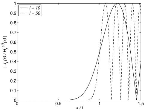
Figure 1: The absolute value of the ratio $J_{l}(x)/H_{l}^{(1)}(x)$ as a function of $x/l$ for two cases: $l=10$ and $l=50$. The ratio significantly differs from zero only for $x\gtrsim l$.

Let us start with determining the angular momentum states dominating the autocorrelation function for a given value of $\kappa$. The ratios inside the brackets in Eq. (19), $J_{l}(x)/H_{l}^{(1)}(x)$, are small for $l>x$, since $J_{l}(x)$ has its first maximum at $x\sim l$. (Figure 1 illustrates the latter argument for cases of $l=10$ and $l=50$.) Consequently, the main contribution to the multiple sum in Eq. (19) comes from terms with $l_{i},l_{j},\ldots,l_{s}$ running from $-[\kappa a]$ to $+[\kappa a]$, and $l,l^{\prime}$ running from $-[\kappa\sigma]$ to $+[\kappa\sigma]$, where the square brackets denote the integer part. At the same time, the large argument approximation of the Hankel function arfk ; gradst ,

$$H_{l}^{(1)}(x)\approx\sqrt{\frac{2}{\pi ix}}\exp\left[i\left(x-\frac{\pi l}{2}\right)\right],$$ (20)

holds for

$$x\gg\frac{1}{2}\left(l^{2}-\frac{1}{4}\right).$$ (21)

Therefore, if $\kappa R_{ij}\gg(2\kappa a)^{2}/2$, and $\kappa R_{0i},\kappa R_{s0}\gg(\kappa a+\kappa\sigma)^{2}/2$ we can use this approximation in Eq. (19) to get

$$\begin{split}\langle\phi_{0}&|G_{0}T_{i}G_{0}T_{j}G_{0}\ldots T_{r}G_{0}T_{s}G_{0}|\phi_{0}\rangle\approx-\frac{m}{\hbar^{2}}\left(\frac{i}{2\pi\kappa}\right)^{1/2}\\ &\times\phi_{0}^{*}(\kappa,k_{0};\theta_{0i}-\theta_{k_{0}})\frac{e^{i\kappa R_{0i}}}{\sqrt{R_{0i}}}f_{\kappa}(\theta_{0i}-\theta_{ij})\frac{e^{i\kappa R_{ij}}}{\sqrt{R_{ij}}}\ldots\\ &\times f_{\kappa}(\theta_{rs}-\theta_{s0})\frac{e^{i\kappa R_{s0}}}{\sqrt{R_{s0}}}\phi_{0}(\kappa,k_{0};\theta_{s0}-\theta_{k_{0}}),\end{split}$$ (22)

where

$$f_{\kappa}(\theta)=-\left(\frac{2}{\pi i\kappa}\right)^{1/2}\sum_{l=-\infty}^{+\infty}\frac{J_{l}(\kappa a)}{H_{l}^{(1)}(\kappa a)}e^{il\theta}$$ (23)

is the scattering amplitude joach describing scattering of a quantum particle of energy $E=\hbar^{2}\kappa^{2}/2m$ from a hard disk of radius $a$ at an angle $\theta$.

The approximation given by Eq. (22) is only valid for energies satisfying the conditions (see Eq. (21) and the discussion right below it)

$$\kappa\ll\frac{R_{ij}}{2a^{2}}\>,\frac{2R_{0i}}{(a+\sigma)^{2}}\;\;\;\;\;\mathrm{for}\;\;\;i,j=1,2,3,\ldots,N.$$ (24)

These conditions bear a simple physical meaning. Suppose $R_{ij},R_{0i}\sim R$ and $\sigma\sim a$, then inequalities (24) can be written as $R\gg 2a/\alpha$, with $\alpha=1/\kappa a$. The latter has a meaning of the angle of diffraction of a wave with the wave length $1/\kappa$ on an obstacle of size $a$, so that $2a/\alpha$ represents the estimate of the shadow depth, which is the largest distance over which the geometrical shadow can exist. Then, the conditions (24) simply mean that the scattering system is so dilute that the average separation between scatterers is much greater than the shadow depth for the given particle’s energy. This is equivalent to stating that Eq. (22) is only valid in the diffraction regime, i.e. the diffraction effects prevail over the geometrical shadow, so that no disk scatterer can be screened from the particle by other disks. In the case of a sufficiently dilute scattering system, $R\gg a$, the inequalities (24) are satisfied for a significant range of energies, so that Eq. (22) provides a good approximation of the autocorrelation function for wave packets confined to this energy range.

Equation (22) has an apparent structure. The initial wave packet $|\phi_{0}\rangle$ is propagated through a sequence of free flight and collision events, each of which contributes by a corresponding product term to the expression for the autocorrelation overlap. Indeed, the latter is multiplied by $e^{i\kappa R}/\sqrt{R}$ each time the particle experiences a free flight through some length $R$, and by $f_{\kappa}(\theta)$ each time the particle scatters off a disk at an angle $\theta$. The same wave function construction algorithm was earlier used in reference gasp-II for semiclassical quantization or the three-disk scattering problem. Nevertheless, it is important to note that, at least for the autocorrelation function calculation, this method fails in the true semiclassical limit, $\kappa\to\infty$, due to violation of the conditions given by (24), and is legitimate only in the diffraction regime approximation defined by (24).

A closer examination of Eq. (22) shows that only such initial wave packets that represent particles moving in the vicinity of system’s classical periodic orbits can exhibit a significantly non-zero autocorrelation function for times corresponding to a number of collision events of the counterpart classical particle. To see that, suppose that the wave packet $|\phi_{0}\rangle$ given by Eq. (17) is well localized in momentum space, i.e. the particle’s de Broglie wave length $\lambdabar\equiv 1/k_{0}\ll\sigma$ . Then, the overlap given by Eq. (22) is negligible unless $\theta_{0i}\approx\theta_{s0}\approx\theta_{k_{0}}$. Indeed, $\phi_{0}(k,k_{0};\theta)$, if considered as a function of the angle $\theta$ between the wave vectors ${\bf{k}}$ and ${\bf{k}}_{0}$, is sharply peaked at $\theta=0$, and rapidly vanishes as ${\bf{k}}$ turns away from ${\bf{k}}_{0}$. This means that the autocorrelation overlap $\langle\phi_{0}|G|\phi_{0}\rangle$ gets a significant scattering contribution in addition to its free-streaming part, $\langle\phi_{0}|G_{0}|\phi_{0}\rangle$, (which is negligible for dilute systems) only if the wave packet is initially located on and moves along a line connecting centers of any two disks in the scattering system. This happens because the reflection wave produced by a disk at the last scattering interferes destructively with the initial wave unless the two waves have their wave vectors pointing almost in the same direction. Hence, one can expect substantially non-zero values of the autocorrelation function only for such initial wave packets that represent classical particles moving along lines connecting scatterer centers, and therefore traveling in the vicinity of unstable periodic orbits of the hard-disk scattering system.

We will now use the propagator given by Eqs. (7) and (22) to calculate the autocorrelation function for the circular wave packet defined in Eq. (17) in three different scattering systems: two-disk, three-disk equilateral and three-disk isosceles billiards. The autocorrelation overlap in the energy domain can be written as

$$\Omega(E)=\langle\phi_{0}|G|\phi_{0}\rangle=\Omega_{0}(E)+\Omega_{\mathrm{S}}(E),$$ (25)

where $\Omega_{0}(E)=\langle\phi_{0}|G_{0}|\phi_{0}\rangle$ is the free flight part of the overlap, and the scattering part, $\Omega_{\mathrm{S}}(E)$, is determined by all possible collision events:

$$\begin{split}\Omega_{\mathrm{S}}(E)&=\sum_{j}\langle\phi_{0}|G_{0}T_{j}G_{0}|\phi_{0}\rangle\\ &+\sum_{j}\sum_{k\neq j}\langle\phi_{0}|G_{0}T_{j}G_{0}T_{k}G_{0}|\phi_{0}\rangle\\ &+\sum_{j}\sum_{k\neq j}\sum_{l\neq k}\langle\phi_{0}|G_{0}T_{j}G_{0}T_{k}G_{0}T_{l}G_{0}|\phi_{0}\rangle+\ldots.\end{split}$$ (26)

The series in Eq. (26) can be summed explicitly for the three above-mentioned billiard systems using the diffraction regime approximation, Eq. (24), together with the assumption of that the initital wave packet has sufficiently high energy, as will be described below.

II.4 Two-disk billiard

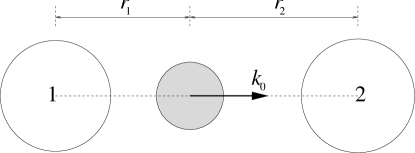
Figure 2: Two-disk billiard. The circular wave packet is initially located on the classical periodic orbit distance $r_{1}$ away from the center of disk “1”, and distance $r_{2}$ away from the center of disk “2”, with $r_{1}+r_{2}=R$.

The simplest of all hard disk systems is the two-disk billiard, which consists of two hard disks, “1” and “2”, of radius $a$ with the center-to-center separation $R$, see fig. 2. Following the discussion above we place the initial wave packet on the line connecting the disk centers with its wave vector ${\bf{k}}_{0}$ pointing along this line in order for the sum in Eq. (26) to have significant, non-vanishing terms. For the initial condition shown in fig. 2 these non-vanishing terms are

$$\begin{split}&\langle\phi_{0}|G_{0}T_{1}G_{0}T_{2}G_{0}\ldots T_{1}G_{0}T_{2}G_{0}|\phi_{0}\rangle\\ &=-\frac{m}{\hbar^{2}}\left(\frac{i}{2\pi\kappa}\right)^{1/2}\left|\phi_{0}(\kappa,k_{0};0)\right|^{2}\\ &\times\frac{e^{i\kappa r_{1}}}{\sqrt{r_{1}}}f_{\kappa}(\pi)\frac{e^{i\kappa R}}{\sqrt{R}}f_{\kappa}(\pi)\frac{e^{i\kappa R}}{\sqrt{R}}\ldots f_{\kappa}(\pi)\frac{e^{i\kappa R}}{\sqrt{R}}f_{\kappa}(\pi)\frac{e^{i\kappa r_{2}}}{\sqrt{r_{2}}},\end{split}$$ (27)

where the diffraction regime approximation, Eq. (22), has been used. Here, $r_{1}$ and $r_{2}$ are the distances separating the center of the wave packet and the centers of disks “1” and “2” respectively; $r_{1}+r_{2}=R$. Substituting Eq. (27) into Eq. (26), while neglecting all other scattering sequences, one obtains a geometric series that sums to

$$\Omega_{\mathrm{S}}(E)=\frac{m}{\hbar^{2}}\left(\frac{iR}{2\pi\kappa r_{1}r_{2}}\right)^{1/2}\frac{\left|\phi_{0}(\kappa,k_{0};0)\right|^{2}}{1-\left(f_{\kappa}(\pi)\dfrac{e^{i\kappa R}}{\sqrt{R}}\right)^{-2}}.$$ (28)

Equation (24) along with the assumption $r_{1}\sim r_{2}\sim R/2$ shows that the validity of the result predicted by Eq. (28) is limited to the energies satisfying $\kappa\ll R/2a^{2},R/(a+\sigma)^{2}$. Now, if the wave packet is sufficiently localized in the momentum space, i.e. the de Broglie wave length

$$\lambdabar\equiv 1/k_{0}\ll\sigma,$$ (29)

and if $k_{0}\ll R/2a^{2},R/(a+\sigma)^{2}$, then Eq. (28) can be used to calculate the time domain autocorrelation function for the wave packet.

Finally we make an assumption that the quantum particle is highly energetic, so that its de Broglie wave length is much smaller than the scatterer size, i.e. $\lambdabar\ll a$. This approximation allows us to use the semiclassical (WKB) expression for the hard-disk scattering amplitude, namely

$$f_{\kappa}(\theta)=-\sqrt{\frac{a}{2}|\sin(\theta/2)|}\>e^{-2i\kappa a|\sin(\theta/2)|}.$$ (30)

Equation (30) is known to be a good approximation of the exact scattering amplitude for sufficiently large scattering angles nuss . Then, combining the diffraction approximation, Eq. (24), with the short de Broglie wavelength approximation, $\lambdabar\ll a$, we arrive at the following condition:

$$\frac{2a^{2}}{R},\dfrac{(a+\sigma)^{2}}{R}\ll\lambdabar\ll a.$$ (31)

We refer to this inequality as to the condition of the high-energy diffraction regime. In the rest of this paper we assume that both the momentum space localization condition, Eq. (29), and the high-energy diffraction regime condition, Eq. (31), are satisfied.

The calculation of the autocorrelation function in the time domain, $C(t)$, is carried out in accordance with Eqs. (13), (14), (25) and (28). The scattering part of the time-domain autocorrelation amplitude reads

$$\Omega_{\mathrm{S}}(t)=\frac{i}{2\pi}\frac{\hbar^{2}}{m}\int_{\Gamma}d\kappa\kappa\exp\left(-i\frac{\hbar t}{2m}\kappa^{2}\right)\Omega_{\mathrm{S}}(E),$$ (32)

where $\Omega_{\mathrm{S}}(E)$ is given by Eq. (28), and contour $\Gamma$ in the complex $\kappa$-plane follows the imaginary axis from $-i\infty$ to $0$, then turns at the right angle, and proceeds to $+\infty$ along the real axis.

Careful analytical calculation of a range of times, for which Eq. (32), with $\Omega_{\mathrm{S}}(E)$ given by Eq. (28), yields accurate predictions, is a formidable problem. Nevertheless, we can use simple physical arguments to roughly estimate this time range. The method that we used to calculate the energy-dependent scattering part of the autocorrelation function, $\Omega_{\mathrm{S}}(E)$, relies on the assumption of the wave packet diffraction. The wave packet must explore the scattering system for the diffraction effects to take place. An estimate of the time needed for the particle to reach the first scatterer is $t_{E}\approx r_{2}/v\sim R/v$, where $r_{2}$ is the distance between the initial location of the particle and the first scatterer it collides with, see fig. 2, and $v=\hbar k_{0}/m$ is the average velocity of the wave packet. Time $t_{E}$ also gives an estimate of the Ehrenfest time for the system: for times shorter than $t_{E}$ the wave packet evolution is dominated by the free particle Hamiltonian, and therefore is classical-like, while particle’s propagation is diffractive and substantially non-classical for times beyond $t_{E}$. To estimate the upper bound of the applicability time-range we note that the WKB expression for the scattering amplitude, Eq. (30), breaks down at low energies $E=\hbar^{2}\kappa^{2}/2m$ with $\kappa\sim 1/a$. The momentum corresponding to these energies is $\hbar\kappa\sim(\lambdabar/a)\hbar k_{0}$, and the corresponding velocity is $v_{\kappa}\sim(\lambdabar/a)v$. The contribution of these low energy modes of the particle to the autocorrelation function become significant after the long wavelength part of the wave packet explores the scattering system, i.e. after times $t_{\max}\sim R/v_{\kappa}\sim(a/\lambdabar)R/v$ corresponding to $a/\lambdabar$ particle-disk collisions. Since $a\gg\lambdabar$ this number of collisions can be quite large. Summarizing, we find that the applicability time-range of our analysis of the time-dependent autocorrelation function is estimated by

$$1\lesssim vt/R\lesssim a/\lambdabar.$$ (33)

In order to evaluate the integral in Eq. (32) one can show that for $t>0$ the contour can be closed along the infinite quarter-circle $\kappa=\kappa_{\infty}e^{i\gamma}$, with $\kappa_{\infty}\to+\infty$, and the angle $\gamma$ decreasing from $0$ to $-\pi/2$ , so that the value of the integral is determined by poles of $\Omega_{\mathrm{S}}(E)$ in the fourth quadrant of the complex $\kappa$ plane:

$$\kappa_{n}=\frac{\pi n}{R}-\frac{i}{2R}\ln\frac{2R}{a},\;\;\;\;\;\;\;\mathrm{for}\;\;\;n=1,2,3,\ldots.$$ (34)

The semiclassical approximation for the scattering amplitude, Eq. (30), was used to find zeros of the denominator of $\Omega_{\mathrm{S}}(E)$, so that Eq. (34) correctly locates the poles right below the region on real $\kappa$ axis where $\phi_{0}(\kappa,k_{0};0)$ is localized. Then, calculating the residues corresponding to the poles, we get

$$\begin{split}&\Omega_{\mathrm{S}}(t)\approx\frac{1}{2}\left(2\pi iRr_{1}r_{2}\right)^{-1/2}\\ &\times\sum_{n\,\sim\,n_{0}-[R/\sigma]}^{n_{0}+[R/\sigma]}\sqrt{\kappa_{n}}\left|\phi_{0}(\kappa_{n},k_{0};0)\right|^{2}\exp\left(-i\frac{\hbar t}{2m}\kappa_{n}^{2}\right),\end{split}$$ (35)

where $\pi n_{0}/R=k_{0}$, and the square brackets in the summation limits represent the integer part. Equation (35) is expected to hold within the time range given by (33).

The free streaming part of the autocorrelation function overlap, $\Omega_{0}(t)=\langle\phi_{0}|G_{0}(t)|\phi_{0}\rangle$, is calculated explicitly for the free particle propagator. It can be shown that its contribution to the full autocorrelation function $C(t)$ is negligible for dilute billiard systems . Therefore, the autocorrelation function for long times is entirely determined by the scattering events, so that $C(t)\approx|\Omega_{\mathrm{S}}(t)|^{2}$.

The main features of the time-domain autocorrelation function $C(t)$ can be deduced by considering only a small number of poles with $n=n_{0}+\tilde{n}$, where $\tilde{n}$ is sufficiently small, so that the pre-exponential function in Eq. (35) stays approximately constant. The contribution due to these poles is

$$\begin{split}\Omega_{\mathrm{S}}(t)&\sim\sum_{\tilde{n}}\exp\left[-i\frac{\hbar t}{2m}\left(k_{0}+\frac{\pi\tilde{n}}{R}-\frac{i}{2R}\ln\frac{2R}{a}\right)^{2}\right]\\ &\sim e^{-iE_{0}t/\hbar}\exp\left(-\frac{1}{2}\lambda^{(2)}t\right)\sum_{\tilde{n}}e^{-i\frac{vt}{R}\pi\tilde{n}},\end{split}$$ (36)

where $E_{0}=\hbar^{2}k_{0}^{2}/2m$ is the average energy of the wave packet, $v=\hbar k_{0}/m$ is its average velocity, and

$$\lambda^{(2)}=\dfrac{v}{R}\ln\dfrac{2R}{a}$$ (37)

is the classical Lyapunov exponent of the two-disk periodic orbit in the limit $R\gg a$, e.g. see reference gasp-book . Equation (36) shows that (i) the envelope of the scattering part of the autocorrelation function decays exponentially with time, $C(t)\sim e^{-\lambda^{(2)}t}$, with the decay rate given by the classical Lyapunov exponent of the system, and (ii) strong interference peaks occur in $C(t)$ at times $t$ multiple to the period of the classical periodic orbit, i.e. when $vt/R$ is an even integer. The peaks of the autocorrelation function correspond to partial reconstruction of the wave packet at times at which the counterpart classical particle returns to its initial point in the phase space.

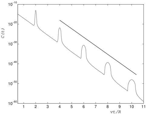
Figure 3: Wave packet autocorrelation function $C(t)$ vs. $vt/R$ for the two-disk billiard. Parameters of the system are as follows: $a=\sigma=1$, $R=10^{4}$, $r_{1}=r_{2}=R/2$ and $\lambdabar=10^{-2}$. The straight line shows exponential decay with the rate given by the classical two-disk Lyapunov exponent $\lambda^{(2)}$. The decay is shown for times $t$ greater than the Ehrenfest time $t_{E}\approx R/2v$.

Figure 3 shows the autocorrelation function, $C(t)$, computed using Eq. (35), with the wave packet given by Eq. (17), for the two-disk billiard with the following parameters: $a=1$ and $R=10^{4}$. The circular wave packet of size $\sigma=1$ is initially placed in the middle between the disks, $r_{1}=r_{2}=R/2$, and its de Broglie wave length $\lambdabar=10^{-2}$. Conditions (29) and (31) are satisfied by this system. The summation in Eq. (35) includes 20,001 poles. The solid line shows $e^{-\lambda^{(2)}t}$ decay. The figure shows the decay for times $t$ greater than the Ehrenfest time $t_{E}\approx R/2v$.

As mentioned above, fig. 3 exhibits the wave packet reconstruction (revival) peaks together with the exponential decay of the autocorrelation function envelope. Another distinct feature of the decay is the broadening of the peaks in the course of time. These phenomena have a simple physical explanation. The direction along the two-disk periodic orbit is neutrally stable, i.e. a perturbation of the initial phase-space point (of a classical particle on the periodic orbit) along this direction growths at most linearly with time. On the other hand, the direction perpendicular to the periodic orbit is exponentially unstable, with the Lyapunov exponent $\lambda^{(2)}$ playing the role of the classical instability rate. Therefore, the wave packet probability density dies out linearly with time in the direction along the periodic orbit, whereas it decreases exponentially in the perpendicular direction . The spreading of the wave packet in the direction along the periodic orbit (and therefore along its average velocity) yields prolongation of time intervals during which $|\phi_{t}\rangle$ significantly overlaps with the initial state $|\phi_{0}\rangle$. This prolongation amounts to broadening of the revival peaks of the autocorrelation function. On the other hand, the wave packet spreading in the unstable direction is responsible for the exponential decay of the autocorrelation function envelope.

II.5 Three-disk systems

We will now calculate the autocorrelation function decay for different scattering systems, namely three-disk billiards, in which a particle moves in two dimensional space with three fixed hard-disk scatterers. Here we restrict ourselves only to such three-disk billiards for which the centers of the disks constitute vertices of an equilateral or of an isosceles triangle. The corresponding scattering systems are then referred to as the three-disk equilateral and isosceles billiards respectively. The discussion of the generic three-disk billiard, in which all three sides of the triangle are different, is left for the Section III.

II.5.1 Three-disk equilateral billiard

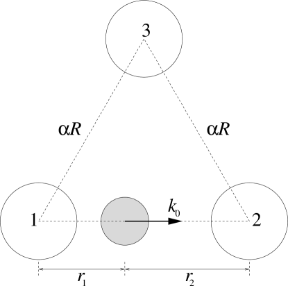
Figure 4: Three-disk isosceles billiard. The circular wave packet is initially located distance $r_{1}$ away from disk “1”, and distance $r_{2}$ away from disk “2”, with $r_{1}+r_{2}=R$. Disk “3” is distance $\alpha R$ away from disks “1” and “2”. The “equilateral” billiard case corresponds to $\alpha=1$.

We consider a geometrically open billiard consisting of three hard disks of radius $a$ centered at the vertices of an isosceles triangle with one side of length $R$ and two other sides of length $\alpha R$, see fig. 4. Here we focus on the case $\alpha=1$, which allows complete analytical treatment. The following section is devoted to the case $\alpha\neq 1$, for which a substantial understanding can be achieved in the limit $\alpha\gg 1$.

As in the case of the two-disk billiard we initially put the wave packet of size $\sigma$ on the line connecting the center of two disks, labeled by “1” and “2”, with center-to-center separation $R$, see fig. 4. Distances $r_{1}$ and $r_{2}$ separating the wave packet center and the centers of disks “1” and “2” respectively satisfy the apparent condition: $r_{1}+r_{2}=R$. The average wave vector of the wave packet ${\bf{k}}_{0}$ is pointing along the line connecting the centers of disks “1” and “2” as shown in fig. 4.

Our calculation of the wave packet autocorrelation function employs the transition matrix method first applied by Gaspard and Rice gasp-II for calculation of scattering resonances in three-disk scattering systems. Transition matrices, and related to them monodromy matrices, have also been used in analysis of different systems by Bogomolny bogom , and Agam and Fishman fish . We fist spell out the multiple collision expansion given by Eq. (26) for the case of a three-disk billiard:

$$\Omega_{\mathrm{S}}(E)=\sum_{n=2}^{\infty}\>\sum_{\mathrm{path}(n)}\langle\phi_{0}|G_{0}T_{1}G_{0}T_{i}G_{0}T_{j}\ldots G_{0}T_{2}G_{0}|\phi_{0}\rangle,$$ (38)

where the second sum runs over all possible paths consisting of $n$ binary collision events with the first collision taking place at disk “2” and the $n^{\mathrm{th}}$ collision at disk “1”. Every term in this double sum is evaluated using the diffraction regime approximation, Eq. (22). Following gasp-II we construct a $6\times 6$ matrix ${\bf Q}$ describing a transition in 6-dimensional space composed of directions $(1\!\to\!2)$, $(1\!\to\!3)$, $(2\!\to\!1)$, $(2\!\to\!3)$, $(3\!\to\!1)$ and $(3\!\to\!2)$, due to a single scattering event,

$${\bf Q}=\begin{array}[]{cc}{}^{1\cdot 2}\;\;{}^{1\cdot 3}\;\;{}^{2\cdot 1}\;\;{}^{2\cdot 3}\;\;{}^{3\cdot 1}\;\;{}^{3\cdot 2}&\\ \left(\begin{array}[]{cccccc}0&0&X&W&0&0\\ 0&0&0&0&X&W\\ X&W&0&0&0&0\\ 0&0&0&0&W&X\\ W&X&0&0&0&0\\ 0&0&W&X&0&0\end{array}\right)&\begin{array}[]{c}\!\!{}^{1\cdot 2}\\ \!\!{}^{1\cdot 3}\\ \!\!{}^{2\cdot 1}\\ \!\!{}^{2\cdot 3}\\ \!\!{}^{3\cdot 1}\\ \!\!{}^{3\cdot 2}\end{array}\end{array}$$ (39)

where

$$X=f_{\kappa}(\pi)\frac{e^{i\kappa R}}{\sqrt{R}}\;\;\;\;\;\mathrm{and}\;\;\;\;\;W=f_{\kappa}(2\pi/3)\frac{e^{i\kappa R}}{\sqrt{R}}.$$ (40)

Here $\pi$ and $2\pi/3$ are the turning angles for a classical particle bouncing among three disk of radius $a$ placed in the vertices of an equilateral triangle with side $R\gg a$. The second sum in Eq. (38) is then given by the one-one element of the matrix ${\bf Q}^{n}$:

$$\begin{split}&\sum_{\mathrm{path}(n)}\langle\phi_{0}|G_{0}T_{1}G_{0}T_{i}G_{0}T_{j}\ldots G_{0}T_{2}G_{0}|\phi_{0}\rangle\\ &\phantom{++}=-\frac{m}{\hbar^{2}}\left(\frac{iR}{2\pi\kappa r_{1}r_{2}}\right)^{1/2}\left|\phi_{0}(\kappa,k_{0};0)\right|^{2}\left({\bf Q}^{n}\right)_{1,1}.\end{split}$$ (41)

Substituting Eq. (41) into Eq. (38), and taking advantage of the equality $\sum_{n=2}^{\infty}{\bf Q}^{n}={\bf Q}^{2}\left({\bf 1}-{\bf Q}\right)^{-1}$, we obtain

$$\begin{split}&\Omega_{\mathrm{S}}(E)=\frac{m}{\hbar^{2}}\left(\frac{iR}{2\pi\kappa r_{1}r_{2}}\right)^{1/2}\left|\phi_{0}(\kappa,k_{0};0)\right|^{2}\\ &\times\left(1-\frac{1/6}{1-W+X}-\frac{1/6}{1-W-X}\right.\\ &\phantom{+++++++++}\left.-\frac{(2+W)/3}{1+W+W^{2}-X^{2}}\right).\end{split}$$ (42)

As in the two-disk billiard case the poles of $\Omega_{\mathrm{S}}(E)$ located in the fourth quadrant of the complex $\kappa$ plane determine the time-domain autocorrelation function. Following gasp-II we define $\xi\equiv-\sqrt{a/R}\>e^{i\kappa R}$ to find that in the limit $R\gg a$ the poles of $S(E)$ are given by

$$\kappa_{n,j}=\frac{2\pi n+\pi+\arg\xi_{j}}{R}-\frac{i}{2R}\ln\frac{R|\xi_{j}|^{2}}{a},$$ (43)

where $j=1,2,3,4$, and

$$\begin{split}&\xi_{1}=\frac{1}{\left(1/2\right)^{1/2}+\left(3^{1/2}/4\right)^{1/2}},\\ &\xi_{2}=\frac{\left(4^{3/2}-3^{3/2}\right)^{1/2}-3^{1/4}}{2\left[1-\left(3/4\right)^{1/2}\right]}\>e^{i\pi},\\ &\xi_{3}=\frac{\left(4^{3/2}-3^{3/2}\right)^{1/2}+3^{1/4}}{2\left[1-\left(3/4\right)^{1/2}\right]},\\ &\xi_{4}=\frac{1}{\left(1/2\right)^{1/2}-\left(3^{1/2}/4\right)^{1/2}}\>e^{i\pi}.\end{split}$$ (44)

Equations (43) and (44), which locate the scattering resonances of the three-disk system, were originally obtained by Gaspard and Rice gasp-II . It is interesting to note that $\kappa_{n2}$ and $\kappa_{n3}$, being the simple poles of the autocorrelation amplitude $\Omega_{\mathrm{S}}(E)$, appear as double poles in the three-disk scattering matrix gasp-II . The three-disk scattering resonances have been also calculated by Cvitanović and Eckhardt cvit by means of the fundamental cycle expansion technique cvit-2 .

The time-domain scattering part of the autocorrelation function, $\Omega_{\mathrm{S}}(t)$, is determined following the procedure used for the analysis of the two-disk billiard system. As before we only consider the poles lying under the region on the real $\kappa$-axis on which the wave packet is mainly concentrated, i.e. $n\in(n_{0}-[R/2\sigma],\,n_{0}+[R/2\sigma])$, with $2\pi n_{0}/R=k_{0}$ and the square brackets denoting the integer part. Calculation of residues of $\Omega_{\mathrm{S}}(E)$ is straightforward. The result is given by

$$\begin{split}&\Omega_{\mathrm{S}}(t)\approx\frac{1}{6}\left(2\pi iRr_{1}r_{2}\right)^{-1/2}\\ &\times\sum_{n\,\sim\,n_{0}-[R/2\sigma]}^{n_{0}+[R/\sigma]}\left\{\sqrt{\kappa_{n1}}\left|\phi_{0}(\kappa_{n1},k_{0};0)\right|^{2}e^{-i\frac{\hbar t}{2m}\kappa_{n1}^{2}}\right.\\ &\phantom{++++++}+2\sqrt{\kappa_{n2}}\left|\phi_{0}(\kappa_{n2},k_{0};0)\right|^{2}e^{-i\frac{\hbar t}{2m}\kappa_{n2}^{2}}\\ &\phantom{++++++}+2\sqrt{\kappa_{n3}}\left|\phi_{0}(\kappa_{n3},k_{0};0)\right|^{2}e^{-i\frac{\hbar t}{2m}\kappa_{n3}^{2}}\\ &\left.\phantom{++++++}+\sqrt{\kappa_{n4}}\left|\phi_{0}(\kappa_{n4},k_{0};0)\right|^{2}e^{-i\frac{\hbar t}{2m}\kappa_{n4}^{2}}\right\}.\end{split}$$ (45)

In order to predict the main features of the decay one can consider only poles in a small vicinity of the peak of the wave function, $n=n_{0}+\tilde{n}$ with $\tilde{n}\ll n_{0}$. This yields

$$\begin{split}\Omega_{\mathrm{S}}(t)&\sim\left[\left(e^{-\tilde{\gamma}_{1}t/2}+2e^{-\tilde{\gamma}_{3}t/2}\right)e^{-i\frac{vt}{R}\pi}\right.\\ &\left.+2e^{-\tilde{\gamma}_{2}t/2}+e^{-\tilde{\gamma}_{4}t/2}\right]e^{-iE_{0}t/\hbar}\sum_{\tilde{n}}e^{-i\frac{vt}{R}2\pi\tilde{n}},\end{split}$$ (46)

where, as before, $E_{0}$ is the average energy of the wave packet, $v$ is its average velocity, and $\tilde{\gamma}_{j}=(v/R)\ln(R|\xi_{j}|^{2}/a)$ with $j=1,2,3,4$. The slowest decay rate, $\tilde{\gamma}_{1}$, playing the role of the decay rate of the autocorrelation function envelope, can be written as

$$\gamma^{(3)}\equiv\tilde{\gamma}_{1}=\dfrac{v}{R}\ln\dfrac{4R}{\left[2^{1/2}+3^{1/4}\right]^{2}a}\approx\dfrac{v}{R}\ln\dfrac{0.54R}{a}.$$ (47)

Once again neglecting the free-streaming amplitude $\Omega_{0}(t)$ we calculate the autocorrelation function as $C(t)\approx|\Omega_{\mathrm{S}}(t)|^{2}$. As in the two-disk billiard case $C(t)$ exhibits a sequence of strong wave packet revival peaks corresponding to phase space returns of the counterpart classical particle, see fig. 5. Taking into account that $|\xi_{1}|\approx 0.73$, $|\xi_{2}|\approx 1.34$, $|\xi_{3}|\approx 11.16$ and $|\xi_{4}|\approx 20.38$ one can notice that the peaks occur whenever $vt/R$ is an integer greater than one, see fig. 5. At $t=R/v$ a part of the wave packet reflected by disk “2” overlaps with the initial wave packet, but this overlap leads to destructive interference since the wave vectors of the two waves have opposite directions. This shows up as the absence of the revival peak at $vt/R=1$, and appears mathematically as partial cancellation of the expression within the square brackets in Eq. (46). It is evident from Eq. (46) together with the inequality $|\xi_{1}|,|\xi_{2}|\ll|\xi_{3}|,|\xi_{4}|$ that, as pointed out by Gaspard and Rice gasp-II , the lines of poles corresponding to $\xi_{3}$ and $\xi_{4}$ are screened by the other two lines of poles and have no affect on the wave packet dynamics. One can also show that after only two collisions the RHS of Eq. (46) becomes totally dominated by the first exponential term within the square brackets resulting in the exponential decay of the autocorrelation function, $C(t)\sim e^{-\gamma^{(3)}t}$.

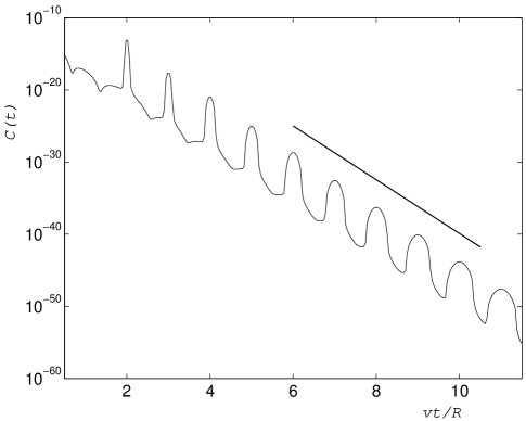
Figure 5: The autocorrelation function vs. $vt/R$ for the three-disk equilateral billiard. Parameters of the system are as follows: $a=\sigma=1$, $R=10^{4}$, $r_{1}=r_{2}=R/2$ and $\lambdabar=10^{-2}$. The straight line shows exponential decay with the rate given by $\gamma^{(3)}$. The decay is shown for times $t$ greater than the Ehrenfest time $t_{E}\approx R/2v$.

Figure 5 shows the decay of the time-dependent autocorrelation function for the three-disk equilateral billiard studied above. The parameters of the system are chosen to be identical with once used in the case of the two-disk billiard: $a=\sigma=1$, $R=10^{4}$, $r_{1}=r_{2}=R/2$ and $\lambdabar=10^{-2}$. The function $C(t)$ for a time interval comprising 10 collision events was calculated by computing the sum in Eq. (45) over the total of 40,006 poles. The straight line shows $e^{-\gamma^{(3)}t}$ decay, with $\gamma^{(3)}$ given by Eq. (47). It is interesting to note how small the magnitude of the autocorrelation function becomes after only a few particle-disk collisions. After the time corresponding to ten bounces of the classical particle, the return probability drops down to a value below $10^{-40}$ implying practical orthogonality of the initial and final states of the quantum particle. It is the consequence of the huge scale difference in the billiard considered here. The phenomenon of the wave packet partial reconstruction can be enhanced by decreasing the ratio $R/a$.

II.5.2 Three-disk isosceles billiard

We now address a more general three-disk scattering system, in which the scatterers are located at the vertices of an isosceles triangle, as shown in fig. 4 with $\alpha\neq 1$. Once again the circular wave packet is initially placed between disks “1” and “2”, which have center-to-center separation $R$, while disk “3” is distance $\alpha R$ away form them, see fig. 4.

The single collision transition matrix ${\bf Q}$, which in the case of an equilateral billiard was given by Eq. (39), now reads

$${\bf Q}=\begin{array}[]{cc}{}^{1\cdot 2}\;\;\;{}^{1\cdot 3}\;\;\;{}^{2\cdot 1}\;\;\;{}^{2\cdot 3}\;\;\;{}^{3\cdot 1}\;\;\;{}^{3\cdot 2}&\\ \left(\begin{array}[]{cccccc}0&0&X_{1}&W_{1}&0&0\\ 0&0&0&0&X_{2}&W_{3}\\ X_{1}&W_{1}&0&0&0&0\\ 0&0&0&0&W_{3}&X_{2}\\ W_{2}&X_{2}&0&0&0&0\\ 0&0&W_{2}&X_{2}&0&0\end{array}\right)&\begin{array}[]{c}\!\!{}^{1\cdot 2}\\ \!\!{}^{1\cdot 3}\\ \!\!{}^{2\cdot 1}\\ \!\!{}^{2\cdot 3}\\ \!\!{}^{3\cdot 1}\\ \!\!{}^{3\cdot 2}\end{array}\end{array}$$ (48)

with

$$\begin{split}&X_{1}=f_{\kappa}(\pi)\frac{e^{i\kappa R}}{\sqrt{R}},\;\;\;\;\;\;\;\;\;\;\;\;X_{2}=f_{\kappa}(\pi)\frac{e^{i\kappa\alpha R}}{\sqrt{\alpha R}},\\ &W_{1}=f_{\kappa}(\pi-\phi_{1})\frac{e^{i\kappa R}}{\sqrt{R}},\;\;\;W_{2}=f_{\kappa}(\pi-\phi_{1})\frac{e^{i\kappa\alpha R}}{\sqrt{\alpha R}},\\ &\phantom{+++++}W_{3}=f_{\kappa}(\pi-\phi_{3})\frac{e^{i\kappa\alpha R}}{\sqrt{\alpha R}}.\end{split}$$ (49)

Here, $\phi_{1}$ and $\phi_{3}$ are angles of the triangle corresponding to vertices “1” and “3” respectively; the angles are functions of $\alpha$, and satisfy the obvious relation: $2\phi_{1}+\phi_{3}=\pi$.

Following the technique used above, we calculate the one-one element of the matrix ${\bf Q}({\bf 1}-{\bf Q})^{-1}$ to obtain the energy dependent autocorrelation function:

$$\begin{split}\Omega_{\mathrm{S}}(E)=&-\frac{m}{\hbar^{2}}\left(\frac{iR}{2\pi\kappa r_{1}r_{2}}\right)^{1/2}\left|\phi_{0}(\kappa,k_{0};0)\right|^{2}\>\frac{\xi^{2}}{\alpha^{2}}\\ &\times\frac{X_{1}^{2}(1-X_{2}^{2})^{2}+\left[2X_{1}X_{2}+W_{3}-X_{2}^{2}(2X_{1}X_{2}-W_{1}W_{2})\right]W_{1}W_{2}-(X_{1}X_{2}-W_{1}W_{2})^{2}W_{3}^{2}}{\left[1-X_{2}^{2}+(X_{1}X_{2}-W_{1}W_{2})W_{3}\right]^{2}-\left[X_{1}(1-X_{2}^{2})+X_{2}(W_{1}W_{2}+W_{3})\right]^{2}}.\end{split}$$ (50)

As above, we introduce $\xi\equiv-\sqrt{a/R}\>e^{i\kappa R}$. The poles of $\Omega_{\mathrm{S}}(E)$, i.e. zeros of the denominator in Eq. (50), are given by solutions of the following two polynomial equations:

$$\begin{split}\left[2-\left(\sqrt{2}-\sqrt{1+\frac{1}{2\alpha}}\right)\xi\right]\xi^{2\alpha}&=\omega_{+}\left(-\frac{a}{R}\right)^{\alpha-1}\left(2-\sqrt{2}\>\xi\right),\\ \left[2+\left(\sqrt{2}-\sqrt{1+\frac{1}{2\alpha}}\right)\xi\right]\xi^{2\alpha}&=\omega_{-}\left(-\frac{a}{R}\right)^{\alpha-1}\left(2+\sqrt{2}\>\xi\right),\end{split}$$ (51)

where

$$\omega_{\pm}=\frac{2\alpha}{1\pm\left(1-\dfrac{1}{4\alpha^{2}}\right)^{1/4}}.$$ (52)

In the limit of $\alpha\to+\infty$ we have $\omega_{+}\to\alpha$ and $\omega_{-}\to 2^{5}\alpha^{3}$.

For the sake of clarity of the following analysis we assume $2\alpha$ to be an integer. Thus, for $R\gg a$ and large $\alpha$ one can find approximate solutions to Eqs. (51):

$$\begin{split}&\xi_{p1}\approx\left(1-\frac{1}{4\alpha}\sqrt{1+\frac{1}{2\alpha}}\>\xi_{p1}^{(0)}\right)\xi_{p1}^{(0)},\\ &\phantom{+++++}\mathrm{with}\;\;\xi_{p1}^{(0)}=\omega_{+}^{1/2\alpha}\left(\sqrt{\frac{a}{R}}\right)^{1-1/\alpha}e^{i\pi(1+p/\alpha)},\\ &\xi_{p2}\approx\left(1+\frac{1}{4\alpha}\sqrt{1+\frac{1}{2\alpha}}\>\xi_{p2}^{(0)}\right)\xi_{p2}^{(0)},\\ &\phantom{+++++}\mathrm{with}\;\;\xi_{p2}^{(0)}=\omega_{-}^{1/2\alpha}\left(\sqrt{\frac{a}{R}}\right)^{1-1/\alpha}e^{i\pi(1+p/\alpha)},\\ &\xi_{3}^{(\pm)}\approx\pm 2\left(\sqrt{2}-\sqrt{1+\dfrac{1}{2\alpha}}\right)^{-1},\end{split}$$ (53)

where $p=1,2,\ldots,2\alpha$. Each of these $4\alpha+2$ values of $\xi$ defines a line of poles of $\Omega_{\mathrm{S}}(E)$ in the complex $\kappa$-plane in accordance with

$$\begin{split}&\kappa_{n,p,j}=\frac{2\pi n+\pi+\arg\xi_{p,j}}{R}-\frac{i}{2R}\ln\frac{R|\xi_{p,j}|^{2}}{a},\\ &\phantom{++++++++++++++++++}\mathrm{with}\;\;j=1,2;\\ &\kappa_{n,3}^{(\pm)}=\frac{2\pi n+\pi+\arg\xi_{3}^{(\pm)}}{R}-\frac{i}{2R}\ln\frac{R|\xi_{3}^{(\pm)}|^{2}}{a}.\end{split}$$ (54)

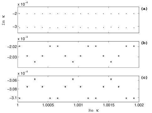
Figure 6: (a) First two “bands” of poles for the case of $\alpha=5/2$ and $R/a=10^{4}$; (b) magnification of the first band; (c) magnification of the second band. Dots correspond to (exact) values of the poles numerically computed directly from Eq. (51), while crosses show the same poles approximated by Eq. (53).

The poles given by Eqs. (54) come in three “bands”. The first and the second bands of poles, corresponding to $\xi_{p,1}$ and $\xi_{p,2}$ respectively, are essential for the wave packet dynamics, while the third band, given by $\xi_{3}^{(\pm)}$, is completely screened by the first two due to the relation $|\xi_{1}|<|\xi_{2}|\ll|\xi_{3}|$. Figure 6 shows the first two bands of poles for the three-disk isosceles billiard with $\alpha=5/2$ and $R/a=10^{4}$. Figure 6a displays the bands over some interval of real $\kappa$-axis, while fig. 6b and fig. 6c magnify the first and the second bands respectively. The dots in the last two figures represent poles numerically computed directly from Eqs. (51), and thus should be thought as of “exact” poles, while crosses are the poles approximated by Eq. (53). In most of the cases the dots and the crosses fall on top of each other, so that one can conclude that Eqs. (53) accurately locate poles of the autocorrelation function.

As we saw earlier, the size of the gap separating the poles and the real $\kappa$-axis determines time decay of the envelope of the autocorrelation function. Thus, the autocorrelation function envelope decay, $C(t)\sim\exp(-\gamma_{\alpha}^{(3)}t)$, for the isosceles three-disk billiard is governed by the rate

$$\gamma_{\alpha}^{(3)}\approx\dfrac{v}{R}\ln\left(\dfrac{R}{a}\left|\xi_{p1}^{(0)}\right|^{2}\right)=\dfrac{v}{\alpha R}\ln\dfrac{2\alpha R}{\left[1+\left(1-\dfrac{1}{4\alpha^{2}}\right)^{1/4}\right]a}.$$ (55)

In the limit $\alpha\gg 1$ the decay rate becomes $\gamma_{\alpha}^{(3)}\approx(v/\alpha R)\ln(\alpha R/a)$.

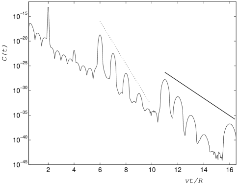
Figure 7: The autocorrelation function as a function of time for the isosceles three-disk billiard with $\alpha=5/2$. Disks “1” and “2” are separated by distance $R=10^{4}a$. The wave packet of the de Broglie wavelength $\lambdabar=10^{-2}a$ is initially located as shown in fig. 4 with $r_{1}=r_{2}=R/2$. The dotted and the solid straight lines represent $e^{-\lambda^{(2)}t}$ and $e^{-\gamma_{\alpha}^{(3)}t}$ decays respectively.

The time-domain autocorrelation function, $C(t)\approx|\Omega_{\mathrm{S}}(t)|^{2}$, is now calculated using Eq. (32), with $\Omega_{\mathrm{S}}(E)$ given by Eq (50). As before, the complex $\kappa$-plane contour integration is performed by calculating the residues of $\Omega_{\mathrm{S}}(E)$ and computing the sum over the poles given by Eq. (54) with the index $n\in(n_{0}-[R/2\sigma],n_{0}+[R/2\sigma])$. Here $2\pi n_{0}/R=k_{0}$ and the square brackets denotes the integer part. The autocorrelation function $C(t)$ for the three-disk isosceles billiard is shown in fig. 7 for the case of $\alpha=5/2$. The system is characterized by $R/a=10^{4}$; the wave packet of the de Broglie wavelength $\lambdabar=10^{-2}a$ is initially placed in the middle between disks “1” and “2”, see fig. 4 with $r_{1}=r_{2}=R/2$. Figure 7 confirms our earlier predictions that the overall envelope of the autocorrelation function decays as $e^{-\gamma_{\alpha}^{(3)}t}$ with the decay exponent $\gamma_{\alpha}^{(3)}$ given by Eq. (55). The trend of this exponential decay is presented by the solid lines in the figure. The dotted trend line corresponds to $e^{-\lambda^{(2)}t}$ decay, with the rate $\lambda^{(2)}$, Eq. (37), being the two-disk Lyapunov exponent of the unstable periodic orbit trapped between disks “1” and “2”.

At first glance the autocorrelation function $C(t)$ appears merely as some complicated sequence of decaying peaks. Nevertheless simple physics underlies its structure. The peaks of the autocorrelation function, or the wave packet partial revivals, occur at instants of time at which the counterpart classical particle returns to its initial point in phase space. Then, relatively larger peaks result from the phase space trajectories with the smaller number of collisions per unit time interval. It is because at every collision event a dominant part of particle’s probability density completely escapes the billiard, and only a tiny part of this density proceeds to the next collision in order to eventually contribute to the autocorrelation function. In other words, phase space periodic orbits with longer mean free paths result in stronger reconstruction peaks. In the isosceles three-disk billiard with $\alpha>1$ the long free flight path trajectories are the ones that pass through disk “3” every second collision, see fig. 4, and return to the initial point at times $t_{n}=(2\alpha n+1)R/v$ with $n=1,2,\ldots$. Thus, $C(t)$ exhibits relatively strong peaks at times $t_{n}$ corresponding to the scattering sequences “132”, “13232”, “13132” etc. During time intervals between the large peaks, i.e. $t_{n-1}<t<t_{n}$, smaller wave packet reconstruction peaks occur due to periodic orbits with shorter mean free paths, which are determined by trajectories bouncing mostly between disks “1” and “2”. This is how the two-disk Lyapunov exponent $\lambda^{(2)}$ enters the description of $C(t)$ for the three-disk billiard. Thus, for times $t<t_{1}$ only the two-disk collision sequences “12”, “1212” etc., contribute to the autocorrelation function, resulting in the $e^{-\lambda^{(2)}t}$ decay.

Another distinctive feature of fig. 7 is the absence of revival peaks for times $R/v$, $3R/v$ and $5R/v$. That is because for a classical particle moving with velocity $v=\hbar k_{0}/m$ there are no phase space periodic orbits corresponding to these times. We have already encountered same phenomenon while discussing the autocorrelation function decay in the three-disk equilateral billiard.

Now it is also apparent how the two-disk decay $e^{-\lambda^{(2)}t}$ is recovered if disk “3” is removed to infinity, see fig. 4. In the limit $\alpha\to\infty$ the time $t_{1}$ of the first large reconstruction peak goes to infinity, resulting in the two-disk billiard decay of the autocorrelation function for $t<t_{1}\to\infty$.

Before closing this section we give a brief summary of the results obtained. We have used the multiple collision expansion technique to provide a detailed first-principle calculation of the time dependent autocorrelation function, $C(t)$, for quantum wave packets moving in billiards composed of two and three hard disk scatterers. By analytically constructing $C(t)$ for three-disk isosceles billiards we have broadened the class of three-disk systems earlier treated by similar methods gasp-II . The applicability limits of these methods were shown to be given by the condition of the high-energy diffraction regime, Eq. (31). We found the decay of the autocorrelation function for the case of a three-disk equilateral billiard to be mainly exponential apart from a regular sequence of wave packet reconstruction peaks of equal relative strength. On the other hand, $C(t)$ decays non-uniformly in the case of a three-disk isosceles system, and features different decay rates at different time scales. Thus, at times shorter that $(2\alpha+1)R/v$, see fig. 4, the decay is entirely determined by the Lyapunov exponent of the shortest two-disk classical periodic orbit, while at long times, the overall envelope decays at a slower rate given by Eq. (55). A well pronounced structure of revival peaks is again observed in the autocorrelation function of the three-disk isosceles billiard. As we will show in the Section III the relative strengths of the peaks are determined by the number of interfering periodic orbits of the counterpart classical system.

III Semiclassical description

In this section we present a simple method for predicting relative strength of the peaks of the wave packet autocorrelation function $C(t)$, see Eq. (1), based on the semiclassical Van Vleck propagator gutz . The semiclassical analysis of the autocorrelation function was earlier performed by Tomsovic and Heller for the case of the stadium billiard toms-2 . We start with applying the semiclassical method for two- and three-disk billiards studied in the previous section, and then, use it to investigate such more complicated scattering systems as the three-disk generic billiard and the two-, three- and four-sphere billiards in three spatial dimensions.

III.0.1 Semiclassical approach

In the limit of short de Boglie wavelengths the time evolution of a quantum state in a hard-disk or hard-sphere billiard can be described by the semiclassical Van Vleck propagator gutz

$$\begin{split}&G_{\mathrm{sc}}({\bf{r}},{\bf{r}}^{\prime};t)\equiv\langle{\bf{r}}|G_{\mathrm{sc}}(t)|{\bf{r}}^{\prime}\rangle\\ &=\left(\frac{1}{2\pi i\hbar}\right)^{d/2}\sum_{\tilde{\gamma}}D_{\tilde{\gamma}}^{1/2}\exp\left(i\frac{S_{\tilde{\gamma}}({\bf{r}},{\bf{r}}^{\prime};t)}{\hbar}-i\frac{\pi\nu_{\tilde{\gamma}}}{2}\right).\end{split}$$ (56)

The summation in this expression goes over all classical paths $\tilde{\gamma}$ connecting points ${\bf{r}}^{\prime}$ and ${\bf{r}}$ (in $d$-dimensional space) in time $t$. $S_{\tilde{\gamma}}({\bf{r}},{\bf{r}}^{\prime};t)$ represents the classical action along the path $\tilde{\gamma}$, and $\nu_{\tilde{\gamma}}$ is an index equal to twice the number of collisions of the particle with hard scatterers during time $t$ gasp-II . The Van Vleck determinant, $D_{\tilde{\gamma}}=|\det(-\partial^{2}S_{\tilde{\gamma}}/\partial{\bf{r}}\partial{\bf{r}}^{\prime})|$, corresponds, up to an appropriate normalization factor, to the classical probability of the path $\tilde{\gamma}$ peres-3 .

The autocorrelation overlap due to the propagator given by Eq. (56) and the an initial quantum state $|\phi_{0}\rangle$ can be written as

$$\langle\phi_{0}|G_{\mathrm{sc}}(t)|\phi_{0}\rangle=\int d{\bf{r}}\int d{\bf{r}}^{\prime}\phi_{0}^{*}({\bf{r}})G_{\mathrm{sc}}({\bf{r}},{\bf{r}}^{\prime};t)\phi_{0}({\bf{r}}^{\prime}),$$ (57)

where asterix denotes complex conjugate. Let us now assume that the wave function $\phi_{0}({\bf{r}})$ is localized about point ${\bf{R}}_{0}$ and has an average momentum $\hbar{\bf{k}}_{0}$,

$$\phi_{0}({\bf{r}})=|\phi_{0}({\bf{r}})|e^{i{\bf{k}}_{0}{\bf{r}}}.$$ (58)

Since both wave functions in the integrand on the right hand side of Eq. (57) are localized about ${\bf{R}}_{0}$, we expand the action $S_{\tilde{\gamma}}({\bf{r}},{\bf{r}}^{\prime};t)$ about the points ${\bf{r}}={\bf{R}}_{0}$ and ${\bf{r}}^{\prime}={\bf{R}}_{0}$ , as

$$S_{\tilde{\gamma}}({\bf{r}},{\bf{r}}^{\prime};t)\approx S_{\gamma}({\bf{R}}_{0},{\bf{R}}_{0};t)+\hbar{\bf{k}}_{\gamma}({\bf{r}}-{\bf{R}}_{0})-\hbar{\bf{k}}^{\prime}_{\gamma}({\bf{r}}^{\prime}-{\bf{R}}_{0}),$$ (59)

where a classical particle traveling along the closed path $\gamma$ would leave the point ${\bf{R}}_{0}$ with momentum $\hbar{\bf{k}}^{\prime}_{\gamma}=-\partial S_{\gamma}({\bf{R}}_{0},{\bf{r}}^{\prime};t)/\partial{\bf{r}}^{\prime}|_{{\bf{r}}^{\prime}={\bf{R}}_{0}}$ and return to ${\bf{R}}_{0}$ after time $t$ having momentum $\hbar{\bf{k}}_{\gamma}=\partial S_{\gamma}({\bf{r}},{\bf{R}}_{0};t)/\partial{\bf{r}}|_{{\bf{r}}={\bf{R}}_{0}}$. Substitution of Eq. (56) along with Eqs. (58) and (59) into Eq. (57) yields

$$\begin{split}&\langle\phi_{0}|G_{\mathrm{sc}}(t)|\phi_{0}\rangle\approx\left(\frac{1}{2\pi i\hbar}\right)^{d/2}\sum_{\gamma}D_{\gamma}^{1/2}\\ &\times\exp\left(i\frac{S_{\gamma}({\bf{R}}_{0},{\bf{R}}_{0};t)}{\hbar}-i\frac{\pi\nu_{\gamma}}{2}\right)[\bar{\phi}_{0}({\bf{k}}_{\gamma})]^{*}\bar{\phi}_{0}({\bf{k}}^{\prime}_{\gamma}),\end{split}$$ (60)

where

$$\bar{\phi}_{0}({\bf{k}})=e^{i{\bf{k}}{\bf{R}}_{0}}\int d{\bf{r}}|\phi_{0}({\bf{r}})|e^{i({\bf{k}}_{0}-{\bf{k}}){\bf{r}}}.$$ (61)

In deriving Eq. (60) we used $D_{\tilde{\gamma}}\approx D_{\gamma}$ and $\nu_{\tilde{\gamma}}=\nu_{\gamma}$ assuming that the paths, $\tilde{\gamma}$ and $\gamma$, are close and follow the same collision sequence.

Let us now assume the function $|\phi_{0}({\bf{r}})|$ to be sufficiently smooth in order for $\bar{\phi}_{0}({\bf{k}})$, defined by Eq. (61), to be sharply peaked about ${\bf{k}}_{0}$. Then, the main contribution to the autocorrelation amplitude in Eq. (60) comes from paths $\gamma$ with ${\bf{k}}_{\gamma}\approx{\bf{k}}^{\prime}_{\gamma}\approx{\bf{k}}_{0}$. Thus, in order to obtain a leading contribution to $\langle\phi_{0}|G_{\mathrm{sc}}(t)|\phi_{0}\rangle$ at a fixed time $t$, one can restrict the summation in Eq. (60) only to classical periodic orbits $\bar{\gamma}$ passing through a small neighborhood of the phase space point $({\bf{R}}_{0},{\bf{k}}_{0})$, and therefore having the momentum $p\approx\hbar k_{0}$. The classical actions along such periodic orbits can be written as $S_{\bar{\gamma}}\approx(\hbar^{2}k_{0}^{2}/2m)\,t$, and are the same for all $\bar{\gamma}$’s. The autocorrelation amplitude then reads

$$\begin{split}\langle\phi_{0}|G_{\mathrm{sc}}(t)|\phi_{0}\rangle&\approx e^{i\frac{\hbar t}{2m}k_{0}^{2}}\left(\frac{1}{2\pi i\hbar}\right)^{d/2}\\ &\times\left(\int d{\bf{r}}|\phi_{0}({\bf{r}})|\right)^{2}\sum_{\bar{\gamma}}D_{\bar{\gamma}}^{1/2}e^{-i\frac{\pi\nu_{\bar{\gamma}}}{2}}.\end{split}$$ (62)

Equation (62) is suitable only for predicting the values of the autocorrelation function $C(t)\approx|\langle|\phi_{0}|G_{\mathrm{sc}}(t)|\phi_{0}\rangle|^{2}$ at times $t=t_{\bar{\gamma}}$ such that there exists at least one classical periodic trajectory $\bar{\gamma}$ of period $t_{\bar{\gamma}}$ passing through the spatial point $R_{0}$ with momentum $\hbar k_{0}$. Due to the narrow momentum distribution of the initial wave packet, given by the function $\bar{\phi}_{0}({\bf{k}})$ in Eq. (60), $C(t)$ decreases by orders of magnitude as the time $t$ changes to a value such that all the classical periodic orbits of period $t$ have momenta different from $\hbar k_{0}$. Therefore, we come to a conclusion that the time decay of the autocorrelation function consists of sequence of sharp peaks centered at the times $t_{\bar{\gamma}}$. Equation (62) is then only suitable for predicting the relative strength and time-location of these peaks.

It will be shown below that the probability measure of periodic orbits (or $D_{\bar{\gamma}}$) decreases exponentially with the increase of the number of collisions a classical particle undergoes while traveling along these orbits. Therefore, the value of the autocorrelation function at a given peak at time $t$ is predominantly determined by a subset $\{\gamma^{\prime}\}$ of the set of all classical periodic trajectories $\{\bar{\gamma}\}$ of length $vt=(\hbar k_{0}/m)t$, such that the members of the subset have the smallest number of scattering events, $N(t)$, possible for time $t$. Indexes $\nu_{\gamma^{\prime}}=2N(t)$ are the same for all members of the subset $\{\gamma^{\prime}\}$, yielding

$$C(t)\sim\left(\sum_{\gamma^{\prime}}\sqrt{D_{\gamma^{\prime}}}\right)^{2}.$$ (63)

Equation (63) allows one to predict the relative magnitude of peaks of the autocorrelation function $C(t)$ by searching (analytically or numerically) for the periodic orbits with the smallest number of scattering events during a given time $t$. We will employ this formula in the sequel to calculate the autocorrelation function decay for wave packets in various hard-disk and hard-sphere billiards.

If properly modified, the above technique is also applicable for calculation of the peaks of the classical autocorrelation function $C_{\mathrm{cl}}(t)$, i.e. a fraction of classical trajectories in a small phase space region around the initial location of a classical particle, which return to this region after time $t$. The classical autocorrelation function gives the phase space return probability for a classical particle described by a phase space distribution function rather by the exact coordinates. It characterizes the escape of classical trajectories from a small neighborhood of a chaotic repeller of the system. In mixing chaotic systems, such as hard-disk and hard-sphere billiards, the autocorrelation function decays exponentially with time, $C_{\mathrm{cl}}(t)\sim e^{-\gamma_{\mathrm{cl}}t}$, with the decay rate $\gamma_{\mathrm{cl}}$ known as the escape rate on the repeller gasp-II ; kantz . The changes one needs to introduce in Eq. (63) are apparent. Due to the absence of interference in classical mechanics one has to directly sum the probabilities of the periodic orbits, $D_{\gamma^{\prime}}$, rather than the probability amplitudes $\sqrt{D_{\gamma^{\prime}}}$. This leads to

$$C_{\mathrm{cl}}(t)\sim\sum_{\gamma^{\prime}}D_{\gamma^{\prime}}.$$ (64)

Finally, one needs to specify quantities $D_{\gamma^{\prime}}$ entering the RHS of Eqs. (63) and (64). This can be done taking into account that the Van Vleck determinant $D_{\gamma^{\prime}}$ equals, up to a normalization factor, the classical probability measure of the trajectory $\gamma^{\prime}$, e.g. see peres-3 . Thus, in $d$-dimensional space the probability density to find a particle at a distance $R$ from the source radiating particles with some initial velocity distribution is proportional to $1/R^{d-1}$. Furthermore, the probability for a particle to undergo a collision with a scatterer in a given direction is described by the differential cross section ${\sigma_{\mathrm{diff}}}(\theta)$, with $\theta$ being the scattering angle. Therefore, the probability for the particle to follow a periodic collision sequence $\eta_{\gamma^{\prime}}=\{i,j,\ldots,q,r,s\}$, constituting an orbit $\gamma^{\prime}$, is

$$\begin{split}D_{\gamma^{\prime}}\sim\frac{{\sigma_{\mathrm{diff}}}(\pi-\phi_{i})}{R_{ij}^{d-1}}&\ldots\frac{{\sigma_{\mathrm{diff}}}(\pi-\phi_{q})}{R_{qr}^{d-1}}\\ &\times\frac{{\sigma_{\mathrm{diff}}}(\pi-\phi_{r})}{R_{rs}^{d-1}}\frac{{\sigma_{\mathrm{diff}}}(\pi-\phi_{s})}{R_{si}^{d-1}},\end{split}$$ (65)

where $R_{ij}$ is the center-to-center separation between scatterers $i$ and $j$, and $\phi_{i}$ is the angle of the periodic orbit polygon (with the vertices at the scatterer centers) corresponding to the $i^{\mathrm{\,th}}$ vertex. The separation distances satisfy an obvious relation,

$$R_{ij}+\ldots+R_{qr}+R_{rs}+R_{si}=vt,$$ (66)

which implicitly provides the time dependents to the RHS of Eqs. (63) and (64).

As we will see below, the expression for the quantum (classical) autocorrelation function proposed in this section, despite its simplicity, accurately predicts times and relative magnitudes of the wave packet (distribution function) reconstruction peaks. Nevertheless, application of more sophisticated techniques, like the one presented in the previous chapter, is required if one needs to obtain absolute (and not relative) values of the autocorrelation function for a wide range of times, including time intervals between the neighboring peaks. One needs to have detailed knowledge of the particle’s wave function in order to predict $C(t)$ for times $t$ other than the peak times, i.e. for times that have no phase space period orbits of velocity $v$ corresponding to them. This requires the construction of the full quantum propagator for a given system by methods analogous to the one presented in Section II.

III.1 Application to studied cases

We first start with applying the semiclassical technique to calculate the peaks of the autocorrelation function for the hard-disk scattering systems analyzed in Section II by the method of multiple collision expansions, i.e. for the two-disk billiard, and three-disk equilateral and isosceles billiards. After that we will treat such more complicated system as the tree-disk generic billiard, as well as some hard-sphere billiards in three dimension.

III.1.1 Two-disk billiard

In the case of the two-disk scattering system, see fig 2, there is only one scattering sequence, “1212$\ldots$”, contributing to a peak of the autocorrelation function, $C(t_{n})$, at time $t_{n}=2nR/v$, with $n=1,2,\ldots$. The probability weight $D_{n}$, corresponding to a periodic orbit of length $vt_{n}$, is calculated according to Eq. (65) with $d=2$ and the semiclassical hard-disk differential cross section

$${\sigma_{\mathrm{diff}}}(\theta)=\frac{a}{2}\left|\sin\frac{\theta}{2}\right|,$$ (67)

where $\theta=\pi$ for the back scattering. Then,

$$C(t_{n})\sim D_{n}\sim\left(\frac{a}{2R}\right)^{2n}=\exp\left(-\lambda^{(2)}t_{n}\right),$$ (68)

where $\lambda^{(2)}$ is the two-disk Lyapunov exponent given by Eq. (37).

Since the right hand sides of Eqs. (63) and (64) reduce to the return probability $D_{n}$ of a single collision sequence, we see that the classical autocorrelation function decays exactly in the same manner as the quantum one:

$$C_{\mathrm{cl}}(t_{n})\sim\exp\left(-\lambda^{(2)}t_{n}\right).$$ (69)

As we will see later, this similarity is the consequence of the fact that the Kolmogorov-Sinai entropy for the two-disk periodic orbit is zero gasp-I , i.e. there is no information production in the system since for any time $t_{n}=2nR/v$ there exists only one trajectory leading to the wave packet (distribution function) partial reconstruction. Thus, the phenomenon of interference between different trajectories is absent in the quantum case, resulting in the same escape rates for classical and semiclassical particles.

III.1.2 Three-disk equilateral billiard

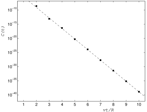
Figure 8: Peaks of the autocorrelation function for the equilateral three-disk billiard calculated in accordance with Eqs. (63), (65) and (67). The dashed line shows $e^{-\gamma^{(3)}t}$ decay, with $\gamma^{(3)}$ given by Eq. (47). The radii of the disks constituting the billiard equal $a=1$, and the disk center-to-center separation is $R=10^{4}$. This figure is to be compared with fig. 5.

Let us now address the three-disk scattering system, with the scatterers centered in the vertices of an equilateral triangle. Figure 8 shows the autocorrelation peaks as a function of time, which were computed numerically according to Eqs. (63), (65) and (67) by summing over all collision sequences satisfying Eq. (66). The dashed trend line in the figure represents the exponential decay with the rate $\gamma^{(3)}$ given by Eq. (47). The billiard is characterized by the disk radius $a=1$, and the disk center-to-center separation $R=10^{4}$. The system is identical to the billiard considered in Section II, see fig. 2, and the decay of the autocorrelation peaks is to be compared with the one presented in fig 3. Note, that the de Broglie wavelength $\lambdabar$ does not enter the sum in Eq. (63), being contained in a possible prefactor, and is therefore not important for determining the relative strength of the peaks. Figure 8 clearly shows that, as in the two-disk case, the semiclassical theory recovers the autocorrelation function decay rate obtained in Section II by means of the multiple collision expansion technique.

The decay rate $\gamma^{(3)}$ given by Eq. (47) for the equilateral three-disk billiard can be exactly recovered using the semiclassical method. In order to calculate $\gamma^{(3)}$ one needs to sum probability amplitudes $\sqrt{D_{\gamma^{\prime}}}$ over all collision sequences $\eta_{\gamma^{\prime}}$ satisfying Eq. (66). Once again, this can be accomplished with the help of the matrix method gasp-II discussed in the previous section. We construct a one-collision transition matrix ${\bf q}$ according to

$${\bf q}=\begin{array}[]{cc}{}^{1\cdot 2}\;{}^{1\cdot 3}\;{}^{2\cdot 1}\;{}^{2\cdot 3}\;{}^{3\cdot 1}\;{}^{3\cdot 2}&\\ \left(\begin{array}[]{cccccc}0&0&x&w&0&0\\ 0&0&0&0&x&w\\ x&w&0&0&0&0\\ 0&0&0&0&w&x\\ w&x&0&0&0&0\\ 0&0&w&x&0&0\end{array}\right)&\begin{array}[]{c}\!\!{}^{1\cdot 2}\\ \!\!{}^{1\cdot 3}\\ \!\!{}^{2\cdot 1}\\ \!\!{}^{2\cdot 3}\\ \!\!{}^{3\cdot 1}\\ \!\!{}^{3\cdot 2}\end{array}\end{array}$$ (70)

with

$$x\equiv\left(\frac{a}{2R}\right)^{1/2}\;\;\;\;\;\;\;\;\mathrm{and}\;\;\;\;\;\;\;\;w\equiv\left(\frac{\sqrt{3}a}{4R}\right)^{1/2}.$$ (71)

Here, $x$ and $w$ are the values of the amplitude $\sqrt{{\sigma_{\mathrm{diff}}}(\pi-\phi)/R}$, with ${\sigma_{\mathrm{diff}}}$ given by Eq. (67) and $\phi$ taking values of $0$ and $\pi/3$ respectively. The matrix ${\bf q}$ describes a transition due to a single collision event in the six-dimensional space spanned by directions $(1\!\to\!2)$, $(1\!\to\!3)$, $(2\!\to\!1)$, $(2\!\to\!3)$, $(3\!\to\!1)$ and $(3\!\to\!2)$. This matrix allows one to express the sum of overlap amplitudes in Eq. (73) for times $t_{n}=nR/v$, with number of collisions $n=2,3,\ldots$, according to

$$\sum_{\gamma^{\prime}}D_{\gamma^{\prime}}^{1/2}(t_{n})=\left({\bf q}^{n}\right)_{1,1},$$ (72)

where the subscript in the RHS denotes that the one-one element of the matrix is taken. The autocorrelation function at the $n^{\,\mathrm{th}}$ collision is related to the one at the $(n+1)^{\,\mathrm{th}}$ collision by

$$\frac{C(t_{n}+R/v)}{C(t_{n})}=\left(\frac{\left({\bf q}^{n+1}\right)_{1,1}}{\left({\bf q}^{n}\right)_{1,1}}\right)^{2}.$$ (73)

For large number of collisions, $n\gg 1$, the largest eigenvalue of the matrix ${\bf q}$, equal to $x+w$, dominates both the numerator and the denominator of Eq. (73), so that

$$\begin{split}&\lim_{t_{n}\to+\infty}\frac{C(t_{n}+R/v)}{C(t_{n})}=(x+w)^{2}\\ &=\frac{a}{R}\left[\left(1/2\right)^{1/2}+\left(3^{1/2}/4\right)^{1/2}\right]^{2}=\exp\left(-\gamma^{(3)}\frac{R}{v}\right),\end{split}$$ (74)

where $\gamma^{(3)}$ is the decay rate given by Eq. (47).

Finally let us mention that the classical escape rate $\gamma_{\mathrm{cl}}^{(3)}$ can be obtained with the help of the transition matrix ${\bf q}$, given by Eq. (70), if one redefines $x$ and $w$ by replacing the square roots in Eq. (71) by the first powers, i.e.

$$x\to\frac{a}{2R}\;\;\;\;\;\mathrm{and}\;\;\;\;\;w\to\frac{\sqrt{3}a}{4R}.$$ (75)

Then,

$$\begin{split}\frac{C_{\mathrm{cl}}(t_{n}+R/v)}{C_{\mathrm{cl}}(t_{n})}&=\frac{\left({\bf q}^{n+1}\right)_{1,1}}{\left({\bf q}^{n}\right)_{1,1}}\;\stackrel{{\scriptstyle t\to\infty}}{{\longrightarrow}}x+w\\ &=\frac{a}{R}\left[\frac{1}{2}+\frac{\sqrt{3}}{4}\right]=\exp\left(-\gamma_{\mathrm{cl}}^{(3)}\frac{R}{v}\right),\end{split}$$ (76)

with the classical escape rate given by

$$\gamma_{\mathrm{cl}}^{(3)}=\frac{v}{R}\ln\frac{4R}{\left[2+\sqrt{3}\right]a}\approx\frac{v}{R}\ln\frac{1.07\,R}{a}.$$ (77)

One can see that the absence of interference in the classical case results in faster particle escape from the scattering system. The classical escape rate for the three-disk equilateral billiard was first obtained by Gaspard and Rice gasp-I .

III.1.3 Three-disk isosceles billiard

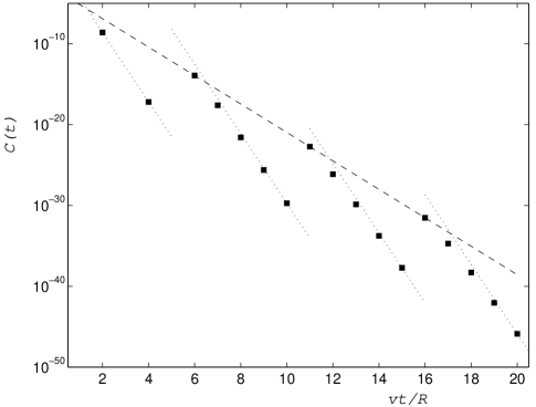
Figure 9: Peaks of the autocorrelation function as predicted by Eq. (63) for the isosceles three-disk billiard with $\alpha=5/2$. The dashed line shows $e^{-\gamma_{\alpha}^{(3)}t}$ decay, with $\gamma_{\alpha}^{(3)}$ given by Eq. (55), while the dotted lines show the trend of the $e^{-\lambda^{(2)}t}$ decay, with $\lambda^{(2)}$ defined by Eq. (37). The billiard is parametrized by $a=1$ and $R=10^{4}$. This figure is to be compared with fig. 7.

In order to complete the comparison of predictions of the semiclassical methods with the results of the detailed binary collision expansion studies, we consider the case of the three-disk billiard with the scatterers centered in the vertices of an isosceles triangle. Figure 9 displays the peaks of the autocorrelation function in the system shown in fig. 4 with $\alpha=5/2$, $a=1$ and $R=10^{4}$. The structure of the decay is twofold. There are relatively big recurrences of the wave packet at times $t_{n}=(2\alpha n+1)R/v=(5n+1)R/v$ with $n=1,2,3,\ldots$. The magnitudes of these recurrences follow $e^{-\gamma_{\alpha}^{(3)}t}$ decay (represented by the dashed line), with the decay rate $\gamma_{\alpha}^{(3)}$ given by Eq. (55). In between any two large neighboring peaks the autocorrelation function decays rapidly, approximately following $e^{-\lambda^{(2)}t}$ decay (dotted lines), with the two-disk Lyapunov exponent $\lambda^{(2)}$ defined by Eq. (37). The sequence of autocorrelation function peaks in fig. 9 is almost identical to the one in fig. 7.

We will now use the matrix method to derive the autocorrelation function envelope decay rate $\gamma_{\alpha}^{(3)}$ directly from Eq. (63). As it was mentioned above the sum in the RHS of Eq. (63) goes only over such periodic orbits $\gamma^{\prime}$ that comprise the smallest number of scattering events possible for a periodic trajectory of length $vt$. This is because the overlap amplitudes $\sqrt{D_{\gamma^{\prime}}}$ corresponding to trajectories with the longest mean free path are given by products of the smallest number of $\sqrt{{\sigma_{\mathrm{diff}}}/R}\ll 1$ terms, and therefore are the dominant ones. In the case of the three-disk isosceles billiard with $\alpha>1$ these long mean free path trajectories are the ones that pass through the scatter “3” every second collision, see fig. 4. This amounts to the collision sequence “132” at time $t_{1}=(2\alpha+1)R/v$, collision sequences “13132” and “13232” at time $t_{2}=(4\alpha+1)R/v$, etc. In general there are $2^{n-1}$ different periodic orbits of length $vt_{n}=(2n\alpha+1)R$ contributing to the autocorrelation function peak $C(t_{n})$.

The relative probability weights of the above trajectories are determined according to Eq. (65) with the differential cross section given by Eq. (67). Thus, collisions $(1\!\to\!3\!\to\!1)$ and $(2\!\to\!3\!\to\!2)$ are described by the cross section ${\sigma_{\mathrm{diff}}}_{3}=a/2$, while $(1\!\to\!3\!\to\!2)$ and $(2\!\to\!3\!\to\!1)$ by ${\sigma_{\mathrm{diff}}}^{\prime}_{3}=(a/2)\cos(\phi_{3}/2)=(a/2)\sqrt{1-1/4\alpha^{2}}$, where $\phi_{3}$ denotes the angle of the triangle corresponding to vertex “3”, see fig. 4. The first and the last collisions of every periodic trajectory deflects the moving particle by the angle $\theta=\pi-\phi_{1}=\pi/2+\phi_{3}/2$, and is described by the cross section ${\sigma_{\mathrm{diff}}}_{1}={\sigma_{\mathrm{diff}}}_{2}=(a/2^{3/2})\sqrt{1+1/2\alpha}$. Here $\phi_{1}$ and $\phi_{2}$($=\!\phi_{1}$) are the other two angles of the isosceles triangle satisfying $2\phi_{1}+\phi_{3}=\pi$. Thus, the sum of overlap amplitudes at time $t_{n}=(2n\alpha+1)R/v$, corresponding to periodic orbits of $2n+1$ collisions, can be written as

$$\sum_{\gamma^{\prime}}D_{\gamma^{\prime}}^{1/2}(t_{n})=\sqrt{\frac{{\sigma_{\mathrm{diff}}}_{1}}{\alpha R}}\>\left({\bf q}^{2n-1}\right)_{1,2}\,\sqrt{\frac{{\sigma_{\mathrm{diff}}}_{2}}{R}},$$ (78)

where

$${\bf q}=\begin{array}[]{cc}{}^{2\cdot 3}\;{}^{3\cdot 1}\;{}^{1\cdot 3}\;{}^{3\cdot 2}&\\ \left(\begin{array}[]{cccc}0&w&0&x\\ 0&0&x&0\\ 0&x&0&w\\ x&0&0&0\end{array}\right)&\begin{array}[]{c}\!\!{}^{2\cdot 3}\\ \!\!{}^{3\cdot 1}\\ \!\!{}^{1\cdot 3}\\ \!\!{}^{3\cdot 2}\end{array}\end{array}$$ (79)

with

$$x\equiv\sqrt{\frac{a}{2\alpha R}}\;\;\;\;\;\mathrm{and}\;\;\;\;\;w\equiv\sqrt{\frac{a}{2\alpha R}}\left(1-\frac{1}{4\alpha^{2}}\right)^{1/4}.$$ (80)

Repeating the arguments used in the case of the three-disk equilateral billiard we find that

$$\begin{split}\frac{C(t_{n+1})}{C(t_{n})}&=\left(\frac{\left({\bf q}^{2n+1}\right)_{1,2}}{\left({\bf q}^{2n-1}\right)_{1,2}}\right)^{2}\stackrel{{\scriptstyle n\to\infty}}{{\longrightarrow}}\>x^{2}(x+w)^{2}\\ &=\left(\frac{a}{2\alpha R}\right)^{2}\left[1+\left(1-\frac{1}{4\alpha^{2}}\right)^{1/4}\right]^{2},\end{split}$$ (81)

since $\sqrt{x(x+w)}$ is the largest eigenvalue of the matrix ${\bf q}$. The time interval between any two successive large peaks of the autocorrelation function is $t_{n+1}-t_{n}=2\alpha R/v$, so that for $n\gg 1$ we get

$$C(t_{n+1})\approx C(t_{n})\exp\left[-\gamma_{\alpha}^{(3)}(t_{n+1}-t_{n})\right],$$ (82)

with the decay rate $\gamma_{\alpha}^{(3)}$ given by Eq. (55). Once again we observe strong agreement between the prediction of the semiclassical analysis and the results of the diffraction regime approximation obtained in Section II.

The classical decay rate $\gamma_{\mathrm{cl},\,\alpha}^{(3)}$ for the three-disk isosceles billiard can be obtained by the following modification of the elements of the transition matrix ${\bf q}$:

$$x\to\frac{a}{2\alpha R}\;\;\;\;\;\mathrm{and}\;\;\;\;\;w\to\frac{a}{2\alpha R}\sqrt{1-\frac{1}{4\alpha^{2}}}\>.$$ (83)

Then,

$$\begin{split}\frac{C_{\mathrm{cl}}(t_{n+1})}{C_{\mathrm{cl}}(t_{n})}&=\frac{\left({\bf q}_{\alpha}^{2n+1}\right)_{1,2}}{\left({\bf q}_{\alpha}^{2n-1}\right)_{1,2}}\stackrel{{\scriptstyle n\to\infty}}{{\longrightarrow}}\>x(x+w)\\ &=\exp\left[-\gamma_{\mathrm{cl},\,\alpha}^{(3)}(t_{n+1}-t_{n})\right],\end{split}$$ (84)

with the classical decay rate

$$\gamma_{\mathrm{cl},\,\alpha}^{(3)}=\frac{v}{\alpha R}\ln\frac{2\alpha R}{\left[1+\sqrt{1-\dfrac{1}{4\alpha^{2}}}\right]^{1/2}a}.$$ (85)

Comparison of Eqs. (55) and (85) shows that, as in the case of the three-disk equilateral billiard, classical particle escape in the isosceles billiard takes place at higher rate than the corresponding quantum process.

III.2 More billiards

As we have seen, the semiclassical method presented here is suitable for predicting the main features of the autocorrelation decay in hard-disk scattering systems. We now apply the method to problems which could not be easily treated by the technique of explicit calculation of scattering resonances used in the Section II.

III.2.1 Generic three-disk billiard

The first system we address is a three-disk billiard of the most general type: the disks of radii $a$ are centered in the vertices of a triangle of unequal sides $R$, $\alpha R$ and $\beta R$, where for concreteness we take $\beta>1,\alpha$. In order to visualize the system one should consider the three-disk isosceles billiard shown in fig. 4, and elongate the side “13” of the triangle from its original length $\alpha R$ to the new length $\beta R$. It is a formidable problem to calculate the scattering resonances (and the corresponding residues) governing the time evolution of a wave packet for such a system. This makes the multiple collision expansion technique, used to study the three-disk equilateral and isosceles billiards, inefficient in the case of the generic three-disk scattering system. On the other hand the semiclassical approach of this section is quite easy to implement. It allows one to extract such important information about the autocorrelation function as the relative strength of the revival peaks and the overall envelope decay rate.

The trajectories with the longest free flight path are the ones that bounce most of their time between disks “1” and “3” with the largest center-to-center separation $\beta R$. In the limit of a large number of collisions, $n\gg 1$, there is a single periodic collision sequence “1313…132” resulting in a relatively strong wave packet recurrence at times $t_{n}=[1+\alpha+(n-2)\beta]R/v$. In accordance with Eqs. (63), (65) and (67) we have

$$\begin{split}C(t_{n})&\sim\left(\frac{a}{2\beta R}\right)^{n-2}\frac{a}{2R}\cos\left(\frac{\phi_{2}}{2}\right)\;\frac{a}{2\alpha R}\cos\left(\frac{\phi_{3}}{2}\right)\\ &\sim\exp\left(-\lambda_{\beta}^{(2)}t_{n}\right),\end{split}$$ (86)

where $\phi_{2}$ and $\phi_{3}$ are the triangle angles at vertices “2” and “3” respectively, and

$$\lambda_{\beta}^{(2)}=\frac{v}{\beta R}\ln\frac{2\beta R}{a}$$ (87)

is the two-disk Lyapunov exponent, see Eq. (37), corresponding to disks “1” and “3”.

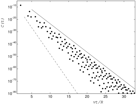
Figure 10: Peaks of the autocorrelation function for the three-disk billiard with $\alpha=\sqrt{2}$, $\beta=2$, $a=1$ and $R=10^{4}$. Solid line represents $e^{-\lambda_{\beta}^{(2)}t}$ decay, with $\lambda_{\beta}^{(2)}$ calculated according to Eq. (87); dashed line corresponds to $e^{-\lambda^{(2)}t}$ decay, with $\lambda^{(2)}$ given by Eq. (37).

Figure 10 shows peaks of the wave packet autocorrelation function for the three-disk billiard with $\alpha=\sqrt{2}$, $\beta=2$, $a=1$ and $R=10^{4}$. The peaks fall inside a narrow cone. Magnitudes of the relatively strongest recurrence peaks decay exponentially with time as $e^{-\lambda_{\beta}^{(2)}t}$, with the decay rate $\lambda_{\beta}^{(2)}$ predicted by Eq. (87). The trend of this exponential decay is shown by the solid line. The dashed line represents the exponential decay $e^{-\lambda^{(2)}t}$ due to the shortest two-disk periodic orbit in the system. The value of $\lambda^{(2)}$ is calculated in accordance with Eq. (37), and represents the fastest decay rate in the billiard.

As shown in Section II, the peaks of the autocorrelation function have significant width which increases with time, see figs. 3, 5 and 7. Therefore, if the autocorrelation function peaks are closely spaced, as in fig. 10, the peak broadening ultimately results in overlapping of neighboring peaks, so that only the overall envelope decay $C(t)\sim e^{\lambda_{\beta}^{(2)}t}$ can be resolved. Thus, the simple semiclassical approach of the section allows one to predict main features of the time-dependent autocorrelation function for wave packets in arbitrary shaped three-disk billiards.

Finally, let us compare the decays of the wave packet autocorrelation function in three-disk scattering systems of three possible types: (i) equilateral ($\alpha=\beta=1$), (ii) isosceles ($\alpha=\beta\neq 1$) and (iii) generic ($\alpha\neq\beta\neq 1$) three-disk billiards. Let also the triangles, constituted by the disks centers, have approximately equal side lengths, and differ only by the number of symmetries. Thus, in the cases (ii) and (iii) both $\alpha$ and $\beta$ are close (but not identical) to unity.

Disk billiard	Decay exponent
$\begin{array}[]{c}\mathrm{Equilateral}\\ \alpha=\beta=1\end{array}$	$\dfrac{v}{R}\ln\dfrac{0.54\,R}{a}$
$\begin{array}[]{c}\mathrm{Isosceles}\\ \alpha=\beta\neq 1\end{array}$	$\dfrac{v}{R}\ln\dfrac{1.04\,R}{a}$
$\begin{array}[]{c}\mathrm{Generic}\\ \alpha\neq\beta\neq 1\end{array}$	$\dfrac{v}{R}\ln\dfrac{2R}{a}$

Table 1: Autocorrelation function decay exponents for three-disk billiards of different symmetries. All billiard are based on almost equilateral triangles, i.e. $\alpha$ and $\beta$ in the second and third row of the table are close to unity.

Table 1 represents the autocorrelation function decay exponents for the above-mentioned three-disk billiards calculated in accordance with Eqs. (47), (55) and (87). One can see that the decay rate increases by approximately $(v/R)\ln\!2$ as the number of equal sides in the three-disk billiard decreases by one. This difference in the decay rates is approximately equal to twice the difference in KS-entropies per unit time of corresponding billiards, and will be discussed in more details in the sequel.

Presence of symmetries in a scattering system increases the number of periodic trajectories of a given length, and thus enhances interference effects. It is due to the interference that strong wave packet reconstruction peaks occur resulting in slower envelope decay of the wave packet autocorrelation function.

III.2.2 Hard-sphere billiards in three dimensions

The above semiclassical approach can also be applied to calculate the autocorrelation function decay for wave packets in three-dimensional hard-sphere billiards. Here we briefly derive the autocorrelation function decay rates for the following three systems: (i) the two-sphere, (ii) the three-sphere equilateral, and (iii) the four-sphere tetrahedral billiards.

The wave packet (phase space distribution) partial reconstruction peaks of the semiclassical (classical) autocorrelation function are given by Eq. (63) (Eq. (64)), with the collision sequences $\eta_{\gamma^{\prime}}$ satisfying Eq. (66). The probability weight $D_{\gamma^{\prime}}$ of the periodic orbits $\gamma^{\prime}$ are now determined from Eq. (65) with $d=3$, and with the differential cross section

$${\sigma_{\mathrm{diff}}}(\theta)=\frac{a^{2}}{4},$$ (88)

where $a$ stands for the radius of the hard-sphere scatterer. It will become clear below that the independence of the differential cross section ${\sigma_{\mathrm{diff}}}$ on the scattering angle $\theta$ significantly simplifies the calculation of the decay rates of $C(t)$ and $C_{\mathrm{cl}}(t)$.

Let us start with analyzing the autocorrelation function peaks for a wave packet moving in a two-sphere billiard consisting of two hard spheres, “1” and “2”, of radius $a$, separated by a distance $R\gg a$, e.g. see fig. 2. A wave packet is initially located on the line connecting the sphere centers and moves toward one of the spheres. As in the two-disk billiard case, there exists only one periodic collision sequence, “1212…”, contributing to the partial wave packet (phase space distribution) reconstruction at times $t_{n}=2nR/v$, with $n=1,2,\ldots$. Hence,

$$C(t_{n})\sim C_{\mathrm{cl}}(t_{n})\sim\left(\frac{a^{2}}{4R^{2}}\right)^{2n}=\exp\left(-\gamma_{\mathrm{3D}}^{(2)}t_{n}\right),$$ (89)

where

$$\gamma_{\mathrm{3D}}^{(2)}=\gamma_{\mathrm{cl,3D}}^{(2)}=2\lambda^{(2)}=\frac{2v}{R}\ln\frac{2R}{a}$$ (90)

is the sum of the two positive Lyapunov exponents, $\lambda^{(2)}=(v/R)\ln(2R/a)$, of the two-sphere periodic orbit. As in the two-disk billiard case, the absence of the interference of different trajectories results in equality of the semiclassical and classical decay rates.

The equilateral three-sphere billiard in three dimensions consists of three spheres of radius $a$ placed in the vertices of an equilateral triangle with side $R\gg a$, e.g. see fig. 4. In this system, the peaks of the autocorrelation function occur at times $t_{n}=nR/v$, with $n=2,3,4,\ldots$ counting the number of collisions. The probability amplitude of a closed paths $\gamma^{\prime}$, given by $\sqrt{D_{\gamma^{\prime}}(t_{n})}=(a/2R)^{n}$, is only a function of time $t_{n}$ and does not depend on the details of the particular collision sequence $\eta_{\gamma^{\prime}}=\{i,j,\ldots,q,r,s\}$ constituting the orbit $\gamma^{\prime}$. The number $M(t_{n})$ of all collision sequences $\eta_{\gamma^{\prime}}$ satisfying Eq. (66) for $t=t_{n}$, and therefore the number of interfering trajectories, can be calculated with the help of the three-dimensional transition matrix

$${\bf q}_{\mathrm{3D}}=\begin{array}[]{cc}\!\!{}^{1\cdot 2}\;{}^{1\cdot 3}\;{}^{2\cdot 1}\;{}^{2\cdot 3}\;{}^{3\cdot 1}\;{}^{3\cdot 2}&\\ \left(\begin{array}[]{cccccc}0&0&1&1&0&0\\ 0&0&0&0&1&1\\ 1&1&0&0&0&0\\ 0&0&0&0&1&1\\ 1&1&0&0&0&0\\ 0&0&1&1&0&0\end{array}\right)&\begin{array}[]{c}\!\!{}^{1\cdot 2}\\ \!\!{}^{1\cdot 3}\\ \!\!{}^{2\cdot 1}\\ \!\!{}^{2\cdot 3}\\ \!\!{}^{3\cdot 1}\\ \!\!{}^{3\cdot 2}\end{array}\end{array}$$ (91)

in accordance with

$$M(t_{n})=\left({\bf q}_{\mathrm{3D}}^{n}\right)_{1,1}.$$ (92)

Here, as above, the subscript “1,1” denotes that the one-one element of the matrix is taken. Then, the magnitude of the autocorrelation function peak at time $t_{n}$ is given by $C(t_{n})\sim[M(t_{n})(a/2R)^{n}]^{2}$. For long times, $n\gg 1$, the decrease of the peak strength due to one collision can be written as

$$\frac{C(t_{n}+R/v)}{C(t_{n})}=\left(\frac{\left({\bf q}_{\mathrm{3D}}^{n+1}\right)_{1,1}}{\left({\bf q}_{\mathrm{3D}}^{n}\right)_{1,1}}\right)^{2}\left(\frac{a}{2R}\right)^{2}\stackrel{{\scriptstyle n\to\infty}}{{\longrightarrow}}\>\left(\frac{a}{R}\right)^{2}.$$ (93)

Here we used that for $n\gg 1$ the ratio of the matrix elements in the last equation is given by the largest eigenvalue of the matrix ${\bf q}_{\mathrm{3D}}$, which is equal to $2$. Therefore, we have

$$C(t_{n})\sim\exp\left(-\gamma_{\mathrm{3D}}^{(3)}\>t_{n}\right),$$ (94)

where

$$\gamma_{\mathrm{3D}}^{(3)}=\frac{2v}{R}\ln\frac{R}{a}$$ (95)

is the autocorrelation function decay rate for the three-sphere equilateral billiard in three dimensions.

The classical decay rate is calculated in the analogous way. According to Eq. (64) we write $C_{\mathrm{cl}}(t_{n})\sim M(t_{n})(a/2R)^{2n}$. Then,

$$\frac{C_{\mathrm{cl}}(t_{n}+R/v)}{C_{\mathrm{cl}}(t_{n})}=\frac{\left({\bf q}_{\mathrm{3D}}^{n+1}\right)_{1,1}}{\left({\bf q}_{\mathrm{3D}}^{n}\right)_{1,1}}\left(\frac{a}{2R}\right)^{2}\stackrel{{\scriptstyle n\to\infty}}{{\longrightarrow}}\>\left(\frac{a}{\sqrt{2}R}\right)^{2},$$ (96)

and consequently

$$C_{\mathrm{cl}}(t_{n})\sim\exp\left(-\gamma_{\mathrm{cl,3D}}^{(3)}\>t_{n}\right),$$ (97)

where

$$\gamma_{\mathrm{cl,3D}}^{(3)}=\frac{2v}{R}\ln\frac{\sqrt{2}R}{a}$$ (98)

is the classical autocorrelation function decay rate of the three-sphere equilateral billiard. Below we will see that the difference between $\gamma_{\mathrm{cl,3D}}^{(3)}$ and $\gamma_{\mathrm{3D}}^{(3)}$ is equal to the topological entropy per unit time (which in this particular system coincides with the KS-entropy per unit time) of the chaotic repeller of the classical system.

Figure 11: The tetrahedral four-sphere billiard. The wave packet is initially placed between spheres “1” and “2”, with its average momentum directed toward sphere “2”.

Finally, we consider a substantially three-dimensional scattering system – a tetrahedral billiard – where four spheres of radius $a$ are placed in the vertices of a pyramid build of four equilateral triangles of sides $R\gg a$. The wave packet starts on a line connecting two disks labeled by “1” and “2”, see fig. 11.

The calculation of the autocorrelation function decay exponent for this billiard proceeds in close analogy with the three-sphere case considered above. The transition matrix $\tilde{{\bf q}}_{\mathrm{3D}}$ is now a $12\times 12$ matrix connecting directions ($1\to 2$), ($1\to 3$), ($1\to 4$), ($2\to 1$), ($2\to 3$), ($2\to 4$), ($3\to 1$), ($3\to 2$), ($3\to 4$), ($4\to 1$), ($4\to 2$) and ($4\to 3$). The structure of the matrix is similar to the one given by Eq. (91) for the case of the three-sphere billiard; the largest eigenvalue is now equal to $3$. As before the number of periodic trajectories contributing to the autocorrelation peak at time $t_{n}=nR/v$, $n=2,3,\ldots$, is given by Eq. (92) with $\tilde{{\bf q}}_{\mathrm{3D}}$ being the $12\times 12$ transition matrix of the four-sphere tetrahedral billiard. Then, the decrease of the autocorrelation function peak strength due to one collision is given by

$$\frac{C(t_{n}+R/v)}{C(t_{n})}=\left(\frac{\left({\bf q}_{\mathrm{3D}}^{n+1}\right)_{1,1}}{\left({\bf q}_{\mathrm{3D}}^{n}\right)_{1,1}}\right)^{2}\left(\frac{a}{2R}\right)^{2}\stackrel{{\scriptstyle n\to\infty}}{{\longrightarrow}}\>\left(\frac{3a}{2R}\right)^{2},$$ (99)

leading to

$$C(t_{n})\sim\exp\left(-\gamma_{\mathrm{3D}}^{(4)}\>t_{n}\right),$$ (100)

with the four-sphere escape decay rate given by

$$\gamma_{\mathrm{3D}}^{(4)}=\frac{2v}{R}\ln\frac{2R}{3a}.$$ (101)

The classical autocorrelation function decay rate for the four-sphere tetrahedral billiard is obtained straightforwardly. According to Eq. (64) we write

$$\frac{C_{\mathrm{cl}}(t_{n}+R/v)}{C_{\mathrm{cl}}(t_{n})}=\frac{\left({\bf q}_{\mathrm{3D}}^{n+1}\right)_{1,1}}{\left({\bf q}_{\mathrm{3D}}^{n}\right)_{1,1}}\left(\frac{a}{2R}\right)^{2}\stackrel{{\scriptstyle n\to\infty}}{{\longrightarrow}}\>\left(\frac{\sqrt{3}a}{2R}\right)^{2}.$$ (102)

This results to

$$C_{\mathrm{cl}}(t_{n})\sim\exp\left(-\gamma_{\mathrm{cl,3D}}^{(4)}\>t_{n}\right),$$ (103)

with

$$\gamma_{\mathrm{cl,3D}}^{(4)}=\frac{2v}{R}\ln\frac{2R}{\sqrt{3}a}.$$ (104)

The semiclassical decay rate, $\gamma_{\mathrm{3D}}^{(4)}$, is again found to be slower than the classical one, $\gamma_{\mathrm{cl,3D}}^{(4)}$. As we will show below the difference between the two decay rates is given by the topological entropy per unit time of the four-sphere tetrahedral billiard repeller.

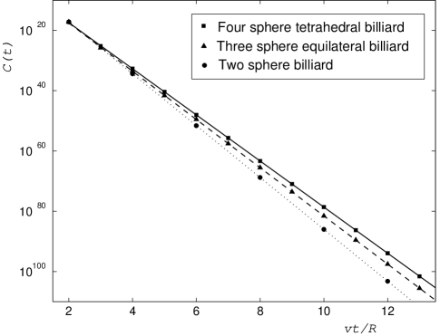
Figure 12: Peaks of the wave packet autocorrelation function for the three scattering systems: two-sphere (circles), three-sphere equilateral (triangles) and four-sphere tetrahedral (diamonds) billiards. In all cases the radius of the sphere scatterers is $a=1$, and the sphere center-to-center separation is $R=10^{4}$. The semiclassical decay rates for these billiards are calculated according to Eqs. (90), (95) and (101), and presented in the figure by the dotted, dashed and solid lines respectively.

Figure 12 shows relative magnitude of peaks of the wave packet autocorrelation function for the three scattering systems considered above: two-sphere, three-sphere equilateral and four-sphere tetrahedral billiards. The radius of the sphere scatterers is $a=1$, and the sphere center-to-center separation is $R=10^{4}$. The semiclassical autocorrelation function decay rates for these billiards are calculated according to Eqs. (90), (95) and (101), and presented in the figure by the dotted, dashed and solid lines respectively. The figure illustrates the reduction of escape of a semiclassical particle from a billiard as additional scatterers are added to the latter. Below we clarify the connection of the rate of this escape to classical properties of the system’s chaotic repeller.

III.3 Classical and semiclassical escape rates

We would now like to comment on the connection of the escapes rates in classical and semiclassical open billiards to such properties of classical chaotic systems as the mean Lyapunov exponents, the Kolmogorov-Sinai (KS) and topological entropy.

The classical escape rate $\gamma_{\mathrm{cl}}$, which is equivalent to the decay rate of the classical autocorrelation function, is known to equal a difference of the stretching and randomization rates in a chaotic system gasp-book ; kantz ; dorf ,

$$\gamma_{\mathrm{cl}}=\sum_{\lambda_{i}>0}\lambda_{i}-h_{\mathrm{KS}}.$$ (105)

Here, the sum, going over all mean positive Lyapunov exponents $\lambda_{i}$, represents the rate of the local exponential stretching of an initial particle phase space distribution, and $h_{\mathrm{KS}}$ is the KS-entropy per unit time of the system characterizing the rate at which the phase space distribution gets randomized over the chaotic repeller of the scattering system. It was first pointed out by Gaspard and Rice gasp-II that the semiclassical escape rate $\gamma$ for the three hard-disk scattering system in two dimensions is given by

$$\gamma\approx\lambda-2h_{\mathrm{KS}},$$ (106)

where $\lambda$ is the mean positive Lyapunov exponent of the corresponding chaotic repeller. Comparison of Eqs. (105) and (106) shows that the semiclassical escape rate is never greater than the escape rate in the counterpart classical system, which is consistent with our observations earlier in this section.

It is interesting to note that the equality in Eq. (106) can be extended (and made exact!) for the three-dimensional hard-sphere billiards considered in this section, i.e. for the two-sphere, three-sphere equilateral and four-sphere tetrahedral scattering systems. Moreover, Eq. (106) can be easily derived for these billiards, since the KS-entropy of the repellers in these systems has an especially simple form. Indeed, the independence of the hard-sphere differential cross section on the scattering angle, evident from Eq. (88), and the equality of lengths of all free flight segments composing the system’s periodic orbit, result in equivalence of probability weights for all trajectories of given length constituting the chaotic repeller, see Eq. (65). Since the probability measure is the same for all periodic trajectories involving a given number of collisions, the construction of the KS-entropy is identical to the construction of the topological entropy, e.g. see dorf . Therefore, for the particular three-dimensional billiards of this section, the KS-entropy per unit time, $h_{\mathrm{KS}}$, of the repeller is simply equal to the topological entropy per unit time, $h_{\mathrm{top}}$. The later is the rate of the exponential growth with time $t$ of the number of different collision sequences, $M(t)$, a classical particle moving on the repeller can possibly undergo:

$$M(t)\sim\exp(h_{\mathrm{top}}\,t).$$ (107)

For the two-sphere billiard there is only one periodic collision sequence a particle staying on the repeller can follow. Thus, $M(t)=1$ and

$$h_{\mathrm{top}}^{(2)}=0.$$ (108)

In the three-sphere equilateral billiard the number of possible trajectories multiplies by two at every collision, so that $M(t)=2^{vt/R}$, leading to

$$h_{\mathrm{top}}^{(3)}=\frac{v}{R}\ln 2.$$ (109)

In the same way we conclude that in the four-sphere tetrahedral billiard the number of possible collision sequences is $M(t)=3^{vt/R}$, so that the topological entropy per unit time reads

$$h_{\mathrm{top}}^{(4)}=\frac{v}{R}\ln 3.$$ (110)

Every trajectory $\gamma^{\prime}$ of the three-dimensional hard-sphere billiard repeller has two positive Lyapunov exponents, $\lambda_{1}(\gamma^{\prime})$ and $\lambda_{2}(\gamma^{\prime})$, corresponding to perturbations of the particle’s initial conditions in two direction perpendicular to the trajectory. It is straightforward to show that the sum of the two Lyapunov exponent, for a dilute hard-sphere scattering system, $R\gg a$, does not depend on the details of the trajectory $\gamma^{\prime}$, and is given by disser

$$\lambda_{1}+\lambda_{2}=\frac{2v}{R}\ln\frac{2R}{a}.$$ (111)

The last equality is obvious for the two-sphere periodic orbit, since in that case $\lambda_{1}=\lambda_{2}=\lambda^{(2)}=(v/R)\ln(2R/a)$. In the case of a general hard-sphere dilute scattering system the method of curvature radii us ; gasp-book can be used to prove Eq. (111).

Looking at the expressions for the classical autocorrelation function decay rates in the three-dimensional billiards studied above, Eqs. (90), (98) and (104), we notice that the following relation holds

$$\gamma_{\mathrm{cl,3D}}^{(j)}=\lambda_{1}+\lambda_{2}-h_{\mathrm{top}}^{(j)},$$ (112)

with $j=2,3,4$. One can also verify that the semiclassical decay rates, given by Eqs. (90), (95) and (101), satisfy

$$\gamma_{\mathrm{3D}}^{(j)}=\lambda_{1}+\lambda_{2}-2h_{\mathrm{top}}^{(j)}.$$ (113)

Equations (112) and (113) are the three-dimensional version of Eqs. (105) and (106) respectively.

The appearance of the factor of $2$ in the expression for the semiclassical decay rate is now apparent: the strength of the wave packet partial reconstruction peaks, $C(t)$, is proportional to $M^{2}(t)$ due to interference of different periodic orbits, while in the classical case $C_{\mathrm{cl}}(t)$ is given merely by the sum of orbit probabilities, and is proportional to $M(t)$. One can also see now that the difference of the two escape rates is given by the topological entropy (which, for the three-dimensional billiards in question, is equal to the KS-entropy) of the chaotic repeller of the classical system, and is therefore determined by underlying classical dynamics.

Figure 13: Schematic picture of a classical periodic orbit $\gamma^{\prime}$ together with an exponentially spreading tube of infinitesimally close trajectories. The initial cross section of the tube, $A_{\gamma^{\prime}}(0)$, gets magnified to the value $A_{\gamma^{\prime}}(t)$, given by Eq. (114), after time $t$ equal to the period of the orbit $\gamma^{\prime}$.

Finally, we would like to further clarify the appearance of the factor of $2$ in the expression for the semiclassical escape rate, Eq. (113), by means of the following simple argument. Consider a classical periodic orbit $\gamma^{\prime}$ of the period $t$, schematically depicted in fig. 13, passing through the phase space point around which the initial wave packet is localized. In a general chaotic system the number of such periodic orbits $M(t)$ grows exponentially with the period $t$, and the rate of this growth is given by the topological entropy per unit time, $h_{\mathrm{top}}$, see Eq. (107). In order to determine the probability weight $D_{\gamma^{\prime}}(t)$ of the orbit $\gamma^{\prime}$, one needs to consider a bundle of trajectories which stay infinitesimally close to $\gamma^{\prime}$. These trajectories form an exponentially thickening tube, see fig. 13, with the initial and final cross sections, $A_{\gamma^{\prime}}(0)$ and $A_{\gamma^{\prime}}(t)$ respectively, related by

$$A_{\gamma^{\prime}}(t)=A_{\gamma^{\prime}}(0)\exp\left(\sum_{\lambda_{j}(\gamma^{\prime})>0}\lambda_{j}(\gamma^{\prime})\>t\right).$$ (114)

Here the sum goes over all positive Lyapunov exponents $\lambda_{j}(\gamma^{\prime})$ of the periodic orbit $\gamma^{\prime}$. Then, the probability for a classical particle taken at random from the trajectory bundle to stay on the periodic orbit $\gamma^{\prime}$ is proportional to the ratio $A_{\gamma^{\prime}}(0)/A_{\gamma^{\prime}}(t)$, so that

$$D_{\gamma^{\prime}}(t)\sim\exp\left(-\sum_{\lambda_{j}(\gamma^{\prime})>0}\lambda_{j}(\gamma^{\prime})\>t\right).$$ (115)

Equation (115) together with (107) leads to the expression for the semiclassical escape rate in the case when the sum over positive Lyapunov exponents, $\sum\lambda_{j}(\gamma^{\prime})$, does not significantly depend on the details of the orbit $\gamma^{\prime}$, and can be replaced by its average value $\sum\lambda_{j}$. Then, the sum over orbits $\{\gamma^{\prime}\}$ in Eq. (63) is simply equal to the product of the number of these orbits, $M(t)$, given by Eq. (107), and the probability amplitude, $\sqrt{D(t)}$, identical for all the orbits and calculated in accordance with Eq. (115). The substitution yields

$$C(t)\sim\left(M(t)\sqrt{D(t)}\right)^{2}\sim\exp\left[-\left(\sum_{\lambda_{j}>0}\lambda_{j}-2h_{\mathrm{top}}\right)\right].$$ (116)

Thus, we recover the expression for the semiclassical autocorrelation function decay rate, Eq. (113), obtained for a number of hard-sphere billiards in three spatial dimensions.

The purpose of the above oversimplified derivation is only to illustrate the origin of the intimate relation between the quantum escape rate and such properties of the underlying classical chaotic system as the Lyapunov exponents and topological (and/or KS) entropy. The details of this relation as well as the limits of its applicability are yet to be investigated.

IV Summary and conclusions

In the first part of this paper we used the technique of multiple collision expansions to construct the quantum propagator for a particle with the de Broglie wavelength, $\lambdabar$, traveling in an array of hard-disk scatterers of radius $a\gg\lambdabar$. The scattering system was assumed to be so dilute that the typical scatterer separation $R$ satisfied the condition $R\gg a^{2}/\lambdabar$. The quantum propagator was used to analytically calculate the time-dependent autocorrelation function for a wave packet, initially localized in both position and momentum spaces, evolving in open two- and three-disk billiard systems. It was found that the autocorrelation function exhibits a sequence of sharp peaks at times multiple to periods of classical phase space periodic orbits of the billiards. These peaks correspond to partial reconstructions of the initial wave packet in the course of its time evolution. The envelope of the correlation function decays exponentially with time after one or two particle-disk collisions; the exponential decay lasts for some $a/\lambdabar\gg 1$ scattering events. Our calculations recovered the autocorrelation function decay rate, first obtained in reference gasp-II , for a particle moving in the three-disk equilateral billiard, and predicted the detailed structure and the decay rate of the autocorrelation function for the more complicated three-disk isosceles billiard.

In the second part of this paper the method of the semiclassical Van Vleck propagator was utilized to derive a simple expression for the relative magnitude of the wave packet partial reconstruction peaks. Although fails to describe the full time dependence of the autocorrelation function, this method allows one to calculate, analytically or numerically, the decay rates of the autocorrelation function envelope (also known as particle escape rates) for much more complicated hard-disk and hard-sphere scattering systems. Here we used it to analyze the three-disk generic billiard, the two-sphere, three-sphere equilateral and three-sphere tetrahedral scattering systems.

A straightforward modification of the semiclassical method allowed us to construct the expression for the peaks of the classical autocorrelation function, and to compare classical and semiclassical particle escape rates in various open hard-disk and hard-sphere billiards. The semiclassical escape rate in three-dimensional scattering systems was shown to be given by the difference of the sum of the two positive Lyapunov exponents and twice the topological entropy (in this case equal to the KS-entropy) per unit time of the underlying classical repeller. Thus, the semiclassical escape rate is never grater then the classical one, and the difference between the two equals to the topological (or KS) entropy per unit time of the classical system. This result is consistent with the earlier findings of reference gasp-II for the case of the two-dimensional hard-disk billiards, and therefore strengthens the connection between classical and quantum chaos.

An interesting seeming “paradox” arises if one compares the expressions for the classical and semiclassical escape rates, e.g. see Eqs. (112) and (113). Indeed, according to the Correspondence Principle it is expected that in the limit of the de Broglie wavelength going to zero the semiclassical escape rate should match its classical counterpart. This seems to be incompatible with the results of this paper: the semiclassical escape rate is expressed in terms of classical quantities only (and does not depend on the de Broglie wavelength), and (in the case of hard-sphere billiards) is smaller than the classical one by the value of the topological entropy of the system. In fact, the difference of the two escape rates originates from noncommutivity of the order in which the infinite time limit and the classical (de Broglie wavelength going to zero) limit are taken. This question has been carefully studied by Barra and Gaspard for the case of quantum graphs barra , as well as discussed in Ref. gasp-IV .

Appendix A Circular wave packet expansion

Here we derive the expansion of the circular wave packet given by Eqs. (17) and (18). The function $\chi_{l}(k,k_{0})$, defined in Eq. (18), can be put in the integral form gradst

$$\chi_{l}(k,k_{0})=\frac{2\sqrt{\pi}}{\sigma}\int_{0}^{\sigma}drrJ_{l}(kr)J_{l}(k_{0}r).$$ (117)

Then,

$$\begin{split}\sum_{l=-\infty}^{+\infty}&\chi_{l}(k,k_{0})e^{il(\theta_{k}-\theta_{k_{0}})}\\ &=\frac{2\sqrt{\pi}}{\sigma}\int_{0}^{\sigma}drr\sum_{l=-\infty}^{+\infty}J_{l}(kr)J_{l}(k_{0}r)e^{il(\theta_{k}-\theta_{k_{0}})}\\ &=\frac{2\sqrt{\pi}}{\sigma}\int_{0}^{\sigma}drrJ_{0}(|{\bf{k}}-{\bf{k}}_{0}|r),\end{split}$$ (118)

where the “summation theorem” for zeroth order Bessel function gradst was used. Doing the simple integral we end up with the equality

$$\sum_{l=-\infty}^{+\infty}\chi_{l}(k,k_{0})e^{il(\theta_{k}-\theta_{k_{0}})}=2\sqrt{\pi}\frac{J_{0}(|{\bf{k}}-{\bf{k}}_{0}|\sigma)}{|{\bf{k}}-{\bf{k}}_{0}|}.$$ (119)

References

- (1) F. Haake, Quantum singnatures of chaos, 2nd Ed. (Springer, Berlin, 2000).
- (2) H. J. Stöckmann, Quantum Chaos: An Introduction, (Cambridge U. Press, Cambridge, 1999).
- (3) M. V. Berry, Ann. Phys. 131, 163 (1980).
- (4) M. Sieber and K. Richter, Phys. Script. T90, 128 (2001).
- (5) H. Primack and U. Smilansky, Phys. Rev. Lett. 74, 4831 (1995); Phys. Rep. 327, 1 (2000).
- (6) P. Gaspard and S. A. Rice, J. Chem Phys. 90, 2225 (1989).
- (7) P. Gaspard and S. A. Rice, J. Chem Phys. 90, 2242 (1989).
- (8) P. Gaspard and S. A. Rice, J. Chem Phys. 90, 2255 (1989).
- (9) P. Gaspard, D. Alonso, T. Okuda, and K. Nakamura, Phys. Rev. E 50, 2591 (1994).
- (10) A. Wirzba, Chaos 2, 77 (1992); A. Wirzba and M. Henseler, J. Phys. A 31, 2155 (1998); A. Wirzba, Phys. Rep. 309, 1 (1999).
- (11) A. Wirzba, “The 1-disk propagator in scalar problems and elastodynamics” (2001), unpublished.
- (12) P. Cvitanović and B. Eckhardt, Phys. Rev. Lett. 63, 823 (1989).
- (13) E. Doran and U. Smilansky, Nonlinearity 5, 1055 (1992); R. Blümel, B. Dietz, C. Jung, and U. Smilansky, J. Phys. A 25, 1483 (1992).
- (14) A. Peres, Ann. Phys. 129, 33 (1980).
- (15) E. J. Heller, E. B. Stechel and M. J. Davis, J. Chem. Phys. 73, 4720 (1980).
- (16) E. J. Heller, Les Houches, Session LII, 1989, Chaos and Quantum Physics, M.-J. Giannoni, A. Voros, and J. Zinn-Justin, eds. (North Holland, Amsterdam, 1991).
- (17) S. Tomsovic and J. H. Lefebvre, Phys. Rev. Lett. 79, 3629, (1997).
- (18) R. W. Robinett, Phys. Rep. 392, 1-119 (2004).
- (19) A. Goussev and J. R. Dorfman, Phys. Rev. E 71, 026225 (2005).
- (20) A. Peres, Phys. Rev. A 30, 1610, (1984).
- (21) T. Prosen, T. H. Seligman and M. Z̆nidaric̆, “Theory of quantum Loschmidt echoes”, quant-ph/0304104.
- (22) R. A. Jalabert and H. M. Pastawski, Phys. Rev. Lett., 86, 2490, (2001); F. M. Cucchietti, H. M. Pastawski, and D. A. Wisniacki, Phys. Rev. E65 045206, (2002); F. M. Cucchietti, C. H. Lewenkopf, E. R. Mucciolo, H. M. Pastawski, and R. O. Vallejos, Phys. Rev. E 65, 046209 (2002); F. M. Cucchietti, H. M. Pastawski, and R. A. Jalabert, Phys. Rev. B 70, 035311 (2004).
- (23) K. M. Watson, Phys. Rev. 105, 1388 (1957).
- (24) C. J. Joachain, Quantum Collision Theory, 3rd Ed. (North Holland, Amsterdam, 1983).
- (25) S. Correia, J. Phys. A 34, 9349 (2001); S. Correia, PhD Dissertation, Universite Louis Pasteur, Strasbourg (2000), webpage http://lpt1.u-strasbg.fr/correia/main_these.ps.gz
- (26) G. B. Arfken and H. J. Weber, Mathematical methods for physicists, 4th Ed., (Academic Press, 1995), pp. 671-674.
- (27) I. S. Gradshteyn and I. M. Ryzhik, Table of integrals, series, and products, 6th Ed., (Academic Press, 2000).
- (28) H. M. Nussenzveig and W. J. Wiscombe, Phys. Rev. A 43, 2093 (1991).
- (29) A. Goussev, PhD Dissertation, University of Maryland, College Park (2005).
- (30) P. Gaspard, Chaos, scattering theory and statistical mechanics, (Cambridge University Press, Cambridge, 1998).
- (31) E. Bogomolny, Nonlinearity 5, 805 (1992); Chaos 2, 5 (1992).
- (32) O. Agam and S. Fishman, J. Phys. A 29, 2013 (1996).
- (33) P. Cvitanović, Phys. Rev. Lett. 61, 2729 (1988).
- (34) M. C. Gutzwiller, Chaos in Classical and Quantum Mechanics, (Springer-Verlag, New York, 1990); M. Brack and R. K. Bhaduri, Semiclassical Physics, (Addison-Wesley, Reading, 1997).
- (35) S. Tomsovic and E. J. Heller, Phys. Rev. E 47, 282 (1993).
- (36) A. Peres, Quantum Theory: Concepts and Methods, (Kluwer Acad. Publ., Dordrecht, 1995).
- (37) H. Kantz and P. Grassberger, Physica D 17, 75 (1985); J.-P. Eckmann and D. Ruelle, Rev. Mod. Phys. 57, 617 (1985).
- (38) J. R. Dorfman, An Introduction to Chaos in Nonequilibrium Statistical Mechanics, (Cambridge University Press, Cambridge, 1999).
- (39) F. Barra and P. Gaspard, Phys. Rev. E 65, 016205 (2001).
- (40) P. Gaspard, NATO ASI Series, Dynamics: Models and Kinetic Methods for Nonequilibrium Many-Body Systems, J. Karkheck, ed. (Kluwer Academic Publishers, Dordrecht, 2000) pp. 425-456.