Synchronization by dynamical relaying in electronic circuit arrays

Abstract

We experimentally study the synchronization of two chaotic electronic circuits whose dynamics is relayed by a third parameter-matched circuit, to which they are coupled bidirectionally in a linear chain configuration. In a wide range of operating parameters, this setup leads to synchronization between the outer circuits, while the relaying element remains unsynchronized. The specifics of the synchronization differ with the coupling level: for low couplings a state of intermittent synchronization between the outer circuits coexists with one of antiphase synchronization. Synchronization becomes in phase for moderate couplings, and for strong coupling identical synchronization is observed between the outer elements, which are themselves synchronized in a generalized way with the relaying element. In the latter situation, the middle element displays a triple scroll attractor that is not possible to obtain when the chaotic oscillator is isolated.

Synchronization of chaos between pairs of coupled dynamical elements has been extensively studied in the last decade. With the recent surge of interest in the collective behaviour of dynamical networks, it has become necessary to determine the conditions in which synchronization persists in the presence of multiple interactions between manifold oscillators. A first nontrivial extension of the two-oscillator case is a linear array of three coupled elements. Here we study experimentally such an architecture with nonlinear electronic elements acting as nodes of the array. Our results show that a pervasive dynamical regime of this system is one in which the outer elements of the chain are synchronized, while the middle one is not, acting merely as a dynamical relay between the two other elements. Depending on the coupling strength, a rich variety of synchronized regimes is observed.

I Introduction

Synchronization between pairs of chaotic systems has been studied profusely in recent years boccaletti02 in fields such as optics uchida05 , driven by potential technological applications, e.g. in secure communications donati02 ; argyris05 . Nonlinear electronic circuits, in particular, have boosted the study and understanding of chaos synchronization, due to their simplicity and the fact that all variables of the circuit are accessible and measurable. Electronic circuits were used, for instance, in pioneering studies on chaotic communications kocarev92 ; cuomo93 .

In this paper we use a particular nonlinear electronic circuit, known as Chua’s circuit or double-scroll oscillator madan93 , which has become a paradigmatic example of chaotic circuit. Chua’s circuit exhibits a rich set of dynamical regimes, ranging from stable to chaotic dynamics, including periodic and excitable behaviors. Moreover, the circuit can be modelled in a straightforward way by a set of three ordinary differential equations. Chaos synchronization between pairs of these circuits has been studied for both unidirectional parlitz00 ; zhu01 and bidirectional canna02 coupling.

Recently, a large interest has appeared in the collective behavior of networks of dynamical elements boccaletti06 . In this context, it is necessary to determine how the network architecture determines the synchronized behavior of coupled chaotic oscillators. Synchronization in large arrays of electronic circuits has already been studied lorenzo96 ; munuzuri99 . But even the simplest extension of the standard two-element system, namely a linear array of three coupled elements, exhibits nontrivial synchronization scenarios. In this paper we investigate experimentally the synchronization regimes of three Chua’s circuits coupled in a linear chain. Coupling is introduced in a bidirectional way, allowing the transfer of information in both directions. In this way, there is not a clear leader in the dynamics neither a system that acts as a simple follower. All circuits influence, in a certain way, the dynamics of the others.

This kind of configuration of three interacting elements has been investigated both theoretically winful90 and experimentally terry99 ; fischer06 in coupled laser systems. Our experimental setup allows a systematic study of the role of coupling in the collective behavior of the system. Our results show that the coupling strength controls different synchronization regimes between the circuits. In all the regimes observed, the central circuit acts as a relay of the dynamics between the two outer ones. In particular, as will be described in detail below, we observe: a) For low coupling levels, intermittent and antiphase synchronization between the outer elements coexist, depending on the initial conditions. b) For moderate coupling, the outer circuits synchronize in phase, their chaotic dynamics being relayed by the central one, which seems to remain unsynchronized. c) For large couplings, the outer lasers are synchronized to each other identically, and to the central one in a generalized way. In that regime, the central circuit exhibits a triple scroll attractor.

II The experimental setup

We focus on the synchronization of three Chua’s circuits coupled in an open-chain configuration. A detailed description of the circuit, with all its components and connections and its corresponding rate equations, is given in Appendix A. As depicted schematically in Fig. 1, a central circuit (B) is coupled to two outer ones (A and C). Voltages $V_{1}$ or $V_{2}$ are sent to the nearest neighbors via a voltage follower, in such a way that a bidirectional link is built upon two unidirectional lines. In other words, each circuit sends out the state of one of its variables, but at the same time receives an input through the other variable (see Appendix B for details).

Figure 1: Schematic representation of the experimental setup.

In this way the circuits are bidirectionally coupled, with the central circuit mediating between the external ones. It is worth noting that the central unit is receiving (sending) two inputs (outputs) while the outer units only receive (send) one. In this sense, one could reasonably expect different dynamics between the central circuit and the outer ones.

The coupling strength is adjusted by a coupling resistance placed between the output of the voltage follower and the input of the receiver circuit. We use a data acquisition card (DAQ) in order to measure the value of $V_{1}$ and $V_{2}$ of each circuit. The DAQ card has a sampling frequency of $50$ KS/s per channel and a maximum input voltage of $\pm 10$ V.

We tune the internal parameters of the circuits so that they exhibit chaotic dynamics in the absence of coupling. Figure 2 displays the evolution of the output variables $V_{1}$ and $V_{2}$ of each isolated circuit [Figs. 2(a) and (b)] and the corresponding phase-space trajectories in the ($V_{1}$,$V_{2}$) plane (Fig. 2c). The dynamics of the isolated circuits corresponds to a single-scroll chaotic attractor.

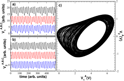
Figure 2: Temporal evolution of $V_{1}$ (a) and $V_{2}$ (b) for the three circuits when coupling strength is set to zero ($R_{\rm coup}\sim\infty$, see Appendix A for details about the circuit design and Appendix B for coupling connections). From top to bottom: A (black), B (red) and C (blue). Voltages have been shifted vertically, in order to ease comparison between time series. (c) Dynamics of circuit A in the phase space given by ($V_{1}$,$V_{2}$). Circuits B and C have similar phase portraits (not shown here).

III The influence of coupling strength

Our aim is to study the influence of coupling strength in the synchronization of the circuit array. Therefore, starting with the three circuits uncoupled, we increase the coupling strength by decreasing the value of the coupling resistances $R_{\rm coup}^{A,B,C}$ placed at the input of each circuit. We keep $R_{\rm coup}^{A}=R_{\rm coup}^{B}=R_{\rm coup}^{C}$ throughout the paper, in order to guarantee the same amount of coupling between all circuits. When $R_{\rm coup}=20$ k$\Omega$ we observe how the circuit outputs begin to modify their dynamics. Specifically, two different behaviors arise, depending on the initial conditions of the array. Figure 3 plots the trajectories in phase space for one of the two possible states. In this case, the two outer circuits (A and C) oscillate in a tight single-scroll attractor, although around two different unstable fixed points. At the same time, the central circuit (B) operates in a double-scroll chaotic attractor. Changes in the dynamics induced by coupling were expected, since they have been recently reported in two bidirectionally coupled Chua’s circuits gomes06 .

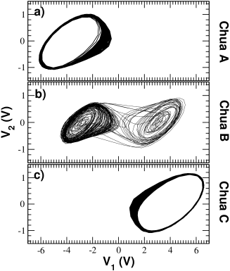
Figure 3: Phase space dynamics of circuits A, B and C for low coupling, corresponding to a coupling resistance $R_{\rm coup}=20$ k$\Omega$.

Figure 4: Temporal evolution of $V_{1}$ (a) and $V_{2}$ (b) of the outer circuits for the situation of Fig. 3 (low coupling): circuit A is shown in black and circuit C in red. The corresponding temporal evolution for circuits A (black) and B (red) is shown in plots (c) and (d).

Figure 4 displays the time series of $V_{1}$ and $V_{2}$ for the three circuits, plotted in pairs for the sake of comparison and keeping $R_{\rm coup}=20$ k$\Omega$. Figures 4(a,b) show the outputs of circuits A and B, which are clearly in antiphase. Furthermore, $V_{1}^{A}$ and $V_{1}^{B}$ have different offsets, a fact that is reflected in the phase space representation (Fig. 3) in the form of oscillations around two different unstable fixed points. Figures 4(c,d) show that circuits A and B remain unsynchronized, a fact also observed for circuits B and C (not shown here). Thus, the central circuit relays a state of antiphase synchronization between the two outer ones, but remains unsynchronized with them.

As we have mentioned above, the antiphase synchronized state described above coexists with another possible behavior of the system. In different realizations of the experiment (corresponding to different initial conditions), the two outer circuits exhibit a double-scroll chaotic attractor, while the central system oscillates in a quasi limit cycle (see the phase space representations in Fig. 5). We note that oscillations at the central circuit exceed the value of $10$ V, which is the limit of the data acquisition card. This fact that does not affect the dynamics of the system, but limits the observable values of $V_{1}$.

Figure 5: Phase space dynamics of circuits A, B and C for low coupling, corresponding to a coupling resistance $R_{\rm coup}=20$ k$\Omega$. The conditions are the same as in Fig. 4, but for a different experimental realization (i.e. different initial conditions), which leads to a different dynamical state.

Figure 6 shows the time series corresponding to the dynamics of Fig. 5, revealing synchronization episodes between the outer circuits A and C [plots (a) and (b)] while the central one performs almost periodic oscillations and remains unsynchronized with the the outer circuits [(c) and (d)]. We ascribe the loss of synchronization between the outer circuits to the interplay between the intrinsic noise of the electronic circuits and the low coupling. As in the previous state, the central Chua acts as a relay between the outer systems in order to achieve synchronization, but it does not participate in the synchronous states between them.

Figure 6: Temporal evolution of $V_{1}$ (a) and $V_{2}$ (b) of the outer circuits for the situation of Fig. 5 (low coupling): circuit A is shown in black and circuit C in red. The corresponding temporal evolution for circuits A (black) and B (red) is shown in plots (c) and (d). The input voltage of the data acquisition card is limited to $10V$.

We now increase coupling strength by reducing the coupling resistance. For $R_{\rm coup}=10$ k$\Omega$, i.e. intermediate coupling, the collective dynamics of the array changes qualitatively. The new situation is depicted in Fig. 7: the central circuit develops a double-scroll chaotic attractor, while the two outer ones exhibit a tight single-scroll attractor. The situation might look similar to the low-coupling case shown in Figs. 3-4, since the two outer circuits oscillate around two different unstable fixed points, while the central system has a different trajectory in phase space. Nevertheless differences arise when looking at the time series, shown in Fig. 8. In this case, circuits A and C remain synchronized in phase [Figs. 8(a,b)], although $V_{1}^{A}$ and $V_{1}^{C}$ have different offsets. This type of synchronized behavior was not observed in the case of low coupling, where the two outer circuits operated in antiphase. Again, the central circuit acts as an information relay, but remains unsynchronized with the two outer circuits [Figs. 8(c,d)].

Figure 7: Phase space dynamics of circuits A, B and C for intermediate coupling, corresponding to a coupling resistance $R_{\rm coup}=10$ k$\Omega$.

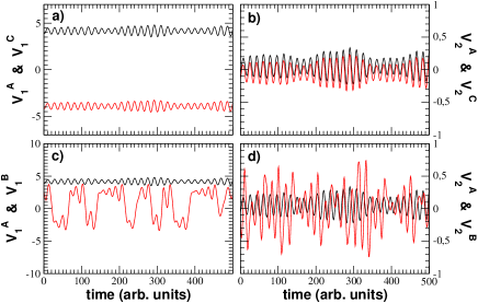
Figure 8: Temporal evolution of $V_{1}$ (a) and $V_{2}$ (b) of the outer circuits for the situation of Fig. 7 (intermediate coupling): circuit A is shown in black and circuit C in red. The corresponding temporal evolution for circuits A (black) and B (red) is shown in plots (c) and (d).

Finally, we increase the coupling even further. For coupling resistances around $R_{\rm coup}\sim 2$ k$\Omega$, which correspond to reasonably high couplings, we observe a new change in the dynamics of the array. Figure 9 shows the phase space portraits of the three coupled circuits in this case. We can see that circuits A and C exhibit a similar double-scroll chaotic attractor. It is worth noting the shape of the chaotic attractor of the central circuit, which is again different from that of the outer ones. In this particular case, however, the central circuit exhibits a triple scroll attractor, a kind of attractor not possible to obtain with an isolated Chua’s circuit. In this way, this kind of bidirectional coupling can be used as a technique to generate different chaotic attractors, as also observed in Ref. zhong98 .

Figure 9: Phase space dynamics of circuits A, B and C for high coupling, corresponding to a coupling resistance $R_{\rm coup}=2$ k$\Omega$.

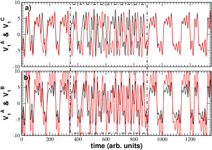
Figure 10: Temporal evolution of $V_{1}$ (a) of the outer circuits (A and C) for the situation of Fig. 9 (high coupling): circuit A is shown in black and circuit C in red. The corresponding temporal evolution for circuits A (black) and B (red) is shown in plot (b). Note the appearance of unsynchronized windows (dotted box) between synchronization regions. Identical synchronization $V_{1}^{A}=V_{1}^{C}$ is obtained in (a), while in (b) we observe generalized synchronization $V_{1}^{B}=aV_{1}^{A}$.

A closer look at the temporal evolution of $V_{1}$ and $V_{2}$ would allow us to explain the appearance of the triple scroll attractor and to decide whether the dynamics of the systems are synchronized or not. Figure 10(a) shows that circuits A and C exhibit identical synchronization, i.e. $V_{1}^{A}=V_{1}^{C}$ (and $V_{2}^{A}=V_{2}^{C}$), coexisting with windows of unsynchronized behaviour. At the same time, synchronization between circuit B (the one with the triple attractor) and the outer ones follows the expression $V_{1}^{B}=aV_{1}^{A}$ (and $V_{2}^{B}=bV_{2}^{A}$), where $a$ (and $b$) is a constant [see synchronization region in Figure 10(b)]. As in the case of the outer circuits, synchronization coexists with states of unsynchronized behaviour and it is during these transients when the system B lies within the central basin of the triple scroll attractor. This kind of synchronization observed between the unsynchronized states, i.e. $V_{1}^{B}=aV_{1}^{A}$, is known as generalized synchronization. The same results are obtained when comparing circuits B and C (not shown here). This is an experimental example of the coexistence of generalized (between the central and outer circuits) and identical synchronization (between the outer circuits) in a chain of coupled chaotic oscillators.

IV Conclusions

In summary, we have investigated the dynamics of three bidirectionally coupled Chua’s circuits, analyzing the influence of the coupling strength in the synchronization of these chaotic oscillators. For low coupling strengths we observe coexistence of two states, which depend on the initial conditions. One state corresponds to antiphase synchronized dynamics at the outer systems, combined with chaotic unsynchronized dynamics with the central one. In the other state we observe episodes of synchronization between the outer systems while the central one has periodic oscillations, and acts as a relay between the two outer systems. For intermediate couplings, generalized synchronization between the outer circuits is obtained, while the central system remains unsynchronized. Finally, for high enough couplings, we observe coexistence of identical synchronization between the outer circuits and generalized synchronization between the central system and the outer ones. Furthermore, we report the appearance of a triple scroll attractor at the central Chua’s circuit, a chaotic attractor not possible to obtain in isolated systems.

Appendix A The Chua’s circuit

Figure 11 shows a detailed description of the Chua’s circuit used in this work. A nonlinear resistor is connected to a set of passive electronic components (R,L,C). We have systematically studied the dynamical ranges of the circuit when $R_{\rm exc}$ is modified, observing stable, periodic, excitable and chaotic dynamics. Among all of them, we drive the circuit to have chaotic dynamics by setting $R_{\rm exc}=1.73$ k$\Omega$. Under these conditions, the dynamics of the circuit in the phase space given by ($V_{1}$,$V_{2}$) lies in a single-scroll chaotic attractor (See Fig. 1). The output of the circuit ($V_{1}$ or $V_{2}$) is sent to the other circuits (with the same characteristics) via a voltage follower, in order to guarantee unidirectional injection (see Appendix B below for details on the coupling implementation).

Figure 11: Description of the Chua circuit, which is built with two TL082 operational amplifiers and passive electronic components of values: $V_{cc}=15$ V, $R_{1}=219.1$ $\Omega$, $R_{2}=21.92$ k$\Omega$, $R_{3}=2.185$ k$\Omega$, $R_{4}=3.28$ k$\Omega$, $R_{L}=23$ $\Omega$, $C_{1}=9.8$ nF, $C_{2}=99.8$ nF, $L=19.54$ mH. We set $R_{\rm exc}=1.73$ k$\Omega$ in order to have chaotic dynamics. $V_{1}$ and/or $V_{2}$ correspond to the outputs of the circuit, which are coupled to the other circuits through a voltage follower.

The dynamics of the circuit are described by the equations kennedy92 :

$$C_{1}\frac{dV_{1}}{dt}=\frac{V_{2}-V_{1}}{R_{e}xc}-g(V_{1},V_{cc})$$ (1)

$$C_{2}\frac{dV_{2}}{dt}=\frac{V_{1}-V_{2}}{R_{e}xc}+I_{L}$$ (2)

$$L\frac{dI_{L}}{dt}=-V_{2}-R_{L}I_{L}$$ (3)

Appendix B Coupling implementation

Figure 12 displays the architecture used to bidirectionally couple the three Chua circuits (schematically described in Fig. 1). For the outer circuits, marked as A and C in Fig. 1, the output variable is $V_{1}$, which is sent to the central circuit (B) through a voltage adder. The coupling strength is controlled by adjusting the value of $R_{8}$. At the same time, $V_{2}$ coming from circuit B is the input variable, which comes trough two voltage followers (one for each outer circuit) and whose strength is adjusted by $R_{7}$ and $R_{6}$. It is worth noting that $R_{8}=R_{7}=R_{6}$ throughout the experiment, in order to keep the same coupling strength between all pairs of circuits.

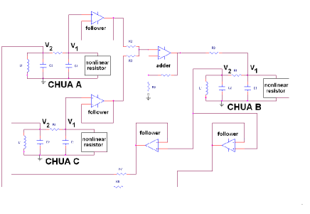
Figure 12: Description of the coupling connections between the three Chua’s circuits. TL082 operational amplifiers are used in the construction of the voltage followers and adders.

References

- (1) S. Boccaletti, J. Kurths, G. Osipov, D. L. Valladares, and C. S. Zhou, “The synchronization of chaotic systems”, Phys. Rep. 366, 1-101 (2002).
- (2) A. Uchida, F. Rogister, J. García-Ojalvo, and R. Roy, “Synchronization and communication with chaotic laser systems”, Prog. Optics 46, 250-341 (2005).
- (3) S. Donati and C.R. Mirasso, “Optical chaos and applications to cryptography”, IEEE J. Quantum Electron. 38, 1138-1140 (2002).
- (4) A. Argyris, D. Syvridis, L. Larger, V. Annovazzi-Lodi, P. Colet, I. Fischer, J. Garc a-Ojalvo, C.R. Mirasso, L. Pesquera and K.A. Shore, “Chaos-based communications at high bit rates using commercial fibre-optic links”, Nature 438, 343 (2005).
- (5) L. Kocarev, K.S. Halle, K. Eckert, L.O. Chua and U. Parlitz, “Experimental demonstration of secure communications via chaotic synchronization”, Int. J. Bifurcation Chaos 2, 709-713 (1992).
- (6) K.M. Cuomo and A.V. Oppenheim, “Circuit implementation of synchronized chaos with applications to communications”, Phys. Rev. Lett. 71, 65-68 (1993).
- (7) R.N. Madan, “Chua’s circuit: A paradigm for chaos” (World Scientific, Singapore, 1993).
- (8) U. Parlitz and I. Wedekind, “Chaotic phase synchronization based on binary coupling signals”, Int. J. Bifurcation Chaos 11, 2527-2532 (2000).
- (9) L. Zhu and Y.-C. Lai, “Experimental observation of generalized time-lagged chaotic synchronization”, Phys. Rev. E 64, 045205(R) (2001).
- (10) B. Canna and S. Cincotti, “Hyperchaotic behaviour of two bidirectionally coupled Chua’s circuits”, Int. J. Circ. Theor. Appl. 30, 625-637 (2002).
- (11) S. Boccaletti, V. Latora, Y. Moreno, M. Chavez, and D.-U. Hwang, “Complex networks: Structure and dynamics”, Phys. Rep. 424, 175-308 (2006).
- (12) M.N. Lorenzo, I.P. Mariño, V. Pérez-Muñuzuri, M.A. Matías, and V. Pérez-Villar, “Synchronization waves in arrays of driven chaotic systems”, Phys. Rev. E 54, 3094-3097 (1996).
- (13) V. Pérez-Muñuzuri and M.N. Lorenzo, “Chaotic synchronization due to multiplicative time-correlated gaussian noise”, Int. J. Bifurcation Chaos 9, 2321-2327 (1999).
- (14) H. G. Winful and L. Rahman, “Synchronized chaos and spatiotemporal chaos in arrays of coupled lasers”, Phys. Rev. Lett. 65, 1575-1578 (1990).
- (15) J. R. Terry, K. S. Thornburg, Jr., D. J. DeShazer, G. D. VanWiggeren, S. Zhu, P. Ashwin and R. Roy, “Synchronization of chaos in an array of three lasers”, Phys. Rev. E 59, 4036-4043 (1999).
- (16) I. Fischer, R. Vicente, J.M. Buldú, M. Peil, C.R. Mirasso, M.C. Torrent, J. Garcia-Ojalvo, “Zero-lag long-range synchronization via dynamical relaying”, preprint nlin.CD/0605036 at http://lanl.arxiv.org
- (17) I. Gomes da Silva, S. Montes, F. d’Ovidio, R. Toral and C. Mirasso, “Coherent regimes of mutually coupled Chua circuits”, Phys. Rev. E 73, 036203 (2006).
- (18) G.-Q. Zhong, C. W. Wu and L. O. Chua, “Torus-doubling bifurcations in four mutually coupled Chua circuits”, IEEE Trans. Circuits Syst. I 45, 186–193 (1998).
- (19) M.P. Kennedy, “Robust OP amp realization of Chua’s circuit,” Frequenz 46, 66–80 (1992).