Reynolds number dependence of drag reduction by rod-like polymers

Abstract

We present experimental and theoretical results addressing the Reynolds number (Re) dependence of drag reduction by sufficiently large concentrations of rod-like polymers in turbulent wall-bounded flows. It is shown that when Re is small the drag is enhanced. On the other hand when Re increases the drag is reduced and eventually the Maximal Drag Reduction (MDR) asymptote is attained. The theory is shown to be in excellent agreement with experiments, rationalizing and explaining all the universal and the non-universal aspects of drag reduction by rod-like polymers.

I Introduction

The phenomenon of turbulent drag reduction describes the increase in the throughput in turbulent flows by adding tiny amounts of polymers. In this way for instance the amount of liquid that is transported in a pipe for a given pressure drop can be increased significantly. This implies a wide range of industrial applications, and consequently the effect, discovered in 1944 by Toms Toms49 , has been studied intensively over the past decades (see e.g. Ref. Virk75a ). The aim of this paper is to rationalize and understand the change from drag enhancement to drag reduction by rod-like polymers in turbulent wall-bounded flows as a function of the Reynolds number Re Book1 ; ASME ; Bonn . To this aim we present new experimental data and a theoretical analysis.

A classical example of the phenomenon of interest is shown in Fig. 1 which pertains to pipe flow ASME . We denote the velocity field ${\bm{U}}({\bm{r}},t)$ and its mean over time as $V(y)$ where $y$ is the distance from the wall. With the mean shear defined as $S(y)\equiv dV(y)/dy$, the Fanning drag coefficient is defined as

$$f\equiv\tau_{w}/\Big{(}\frac{1}{2}\rho\tilde{V}^{2}\Big{)}\ ,$$ (1)

where $\tau_{w}$ is the wall shear stress at the wall

$$\tau_{w}\equiv\rho\nu S(y=0)\ ,$$ (2)

$\nu$, $\rho$ and $\tilde{V}$ are the kinematic viscosity, the fluid density and the mean fluid throughput, respectively. Fig. 1 presents this quantity as a function of Re in the traditional Prandtl-Karman coordinates $1/\sqrt{f}$ vs. Re$\sqrt{f}$. The straight continuous line denoted by ‘N’ presents the Newtonian universal law. Data points below this line are indicative of a drag enhancement, i.e., an increase in the dissipation due to the addition of the polymer. Converesely, data points above the line correspond to drag reduction, which is always bound by the Maximal Drag Reduction (MDR) asymptote represented by the dashed line denoted by ‘M’. This figure shows data for a rod-like polymer (a polyelectrolyte in aqueous solution at very low salt concentration) and shows how drag enhancement for low values of Re crosses over to drag reduction at large values of Re ASME ; Bonn . One of the results of this paper is the theory presented below, that reproduces the phenomena shown in Fig. 1 in a satisfactory manner.

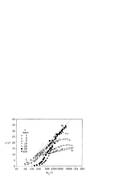
Figure 1: The drag in Prandtl-Kármán coordinates for the water with the rod-like polymer PAMH B1120 in 0.0001N NaCl in a pipe flow, see ASME for details. The symbols represent the concentrations in wppm (weight parts per million) as given in the figure.

It is interesting to note that with flexible polymers the situation is very different, and there is no drag enhancement at any value of Re. The reason for this distinction will be made clear below as well.

In Sec. 2 we present new experimental results in which drag reduction is measured as a function of the Reynolds number, and for different concentrations of the rod-like polymer. We determine the rheological properties of these solutions simultaneously, so that the rheology of the solutions is known. In Sec. 3 we review the basic theoretical approach to drag reduction in general, and by rod-like polymers in particular. We discuss the effect of the polymers on the fluid flow in three cases: high Re flows, low Re flows and intermediate Re flows, respectively. In Sec. 4 we explain how to solve the equations and present the results and their comparison to the experiments. Discussions and the conclusions are presented in Sec. 5.

II Experimental

II.1 Flow Geometry and Polymer

In this section we describe the experimental results obtained using well-characterized rod-like polymer solutions. The turbulence cell has been previously described in detail by Cadot et al.Cadot . A turbulent flow is generated in a closed cylindrical cell (of volume three liters) between two counter-rotating disks spaced one disk diameter apart. The disks are driven by DC motors. The motors are configured to keep the disks rotating at a constant angular velocity $\Omega$, independently of the torque exerted by the turbulent fluid on the disks. Thus, all the experiments presented here are performed at constant angular velocity. All experiments were repeated with pure water and with the water seeded with the polymers. In both cases we define Cadot the integral Reynolds number as Re$=\rho\Omega R^{2}/\eta_{{}_{S}}$, where $\rho$ is the density and $R$ is the radius of the disks. To determine the energy dissipation in the turbulent fluid (from which we also infer the amount of drag reduction or drag enhancement), we take advantage of the fact that we are in a closed system. All the kinetic energy fed into the flow will eventually be dissipated viscously, leading to a temperature increase of the fluid: by measuring the temperature increase in time $\Delta T/\Delta t$ we can also estimate the power dissipated by the turbulent flow. The temperature is measured with a Pt thermocouple probe with an accuracy of $0.01^{\circ}$C. From our temperature measurements, we can then deduce the percentage of drag reduction ($DR$) from:

$$DR(\%)\equiv 100\times\left[1-\frac{(\Delta T/\Delta t)_{\rm poly}}{(\Delta T/\Delta t)_{\rm water}}\right]\ .$$ (3)

For the polymer we use solutions of Xanthane, a stiff rodlike polymer with an average molecular weight of $M_{w}=3.10^{6}{\rm g.mol}^{-1}$. The rheology of the polymer solutions was studied on a Reologica Stress-Tech (cone-plate geometry) rheometer. The latter is equipped with a normal force transducer, and has a large cone (55 mm) with a small angle ($0.4^{\circ}$) in order to be able to detect small normal stress differences at high shear rates. Changing the concentration allows us to modify the shear-dependent viscosity of the solutions. The apparent viscosity decreases with increasing shear rate, i.e., the fluid is shear thinning. A satisfactory description of most of the data for high shear rates can be obtained using the Ostwald-de Waele power law model Bird for the viscosity $\eta$: $\eta=k_{1}S^{(n-1)}$; the viscosity shows a power law dependence on the shear rate $S$. The validity of this model is limited to a certain range of shear rates, depending on the concentration $C$ of the polymer solution; the range and constants $k_{1}$ and $n$ are reported in Lindner . For the whole concentration range studied here ($0<C<2000$ wppm), no measurable normal stresses were found in the range of shear rates studied ($10<S<6000{\rm s}^{-1}$); the uncertainty on the measurements is of the order of 10Pa.

The other important difference in the rheology of the rigid polymers, compared to solutions of flexible polymers, is the elongational viscosity $\eta_{E}$, which quantifies the resistance to stretching of a fluid element. If sufficiently important, $\eta_{E}$ can be measured Drops by looking at droplet fission with a rapid camera (Fig. 2). The dynamics of the thinning of the filament that connects the droplet to the orifice can be used to obtain the elongational viscosity since the stretching of the filament corresponds to a perfectly elongational flow. Performing this experiment, we find that, for the rigid polymer solution, $\eta_{E}$ is so low that the dynamics of the filament is nearly indistinguishable from that of pure water for which $\eta_{E}=$3mPas Trouton .

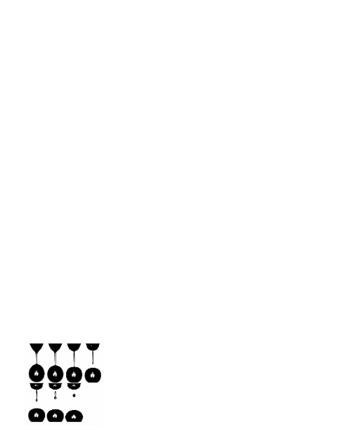
Figure 2: Droplet detachment for a 300 wppm Xanthane solution filmed with a rapid camera: there is 1ms between subsequent images.

II.2 Results

In Fig. 3 the percentage drag reduction $DR(\%)$ is plotted as a function of the Reynolds number for three different polymer concentrations. Also in our measurement geometry and with our rod-like polymer at low $Re$ a drag enhancement is observed, which smoothly transforms into a drag reduction at high Re.

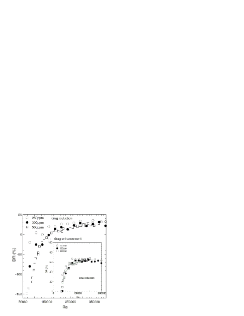
Figure 3: Percentage of drag reduction (or enhancement) vs. Re for three different polymer concentrations. Inset: percentage of drag reduction vs. Re when the actual viscosity (including the polymer) is used in the definition of Re).

In this paper we rationalize and explain the results presented in both Fig. 1 and Fig. 3. To this aim we turn now to a review of the theory of drag reduction.

III Review of the Theory of Drag Reduction by Rod-like polymers

In the presence of a small concentration of rod-like polymers, the Navier-Stokes equations for the fluid velocity ${\bm{U}}({\bm{r}},t)$ gain an additional contribution to the stress tensor:

$$\frac{\partial{\bm{U}}}{\partial t}+{\bm{U}}\cdot{\bm{\nabla}}{\bm{U}} = -\nabla p+\nu_{0}\nabla^{2}{\bm{U}}+\nabla\cdot{{\bm{\sigma}}}\ ,$$ (4)

$$\nabla\cdot{\bm{U}} = 0\ .$$

The extra stress tensor ${\bm{\sigma}}$ is due to the interaction between the polymers and the fluid. For rod-like polymers it takes the form 88DE :

$$\sigma_{ab}=6\nu_{p}n_{a}n_{b}(n_{i}n_{j}\mathcal{S}_{ij})\ ,$$ (5)

where $\nu_{p}$ is the viscosity contributed by the polymer in the limit of zero shear, ${\bm{n}}\equiv{\bm{n}}(t,{\bm{r}})$ is a unit vector describing the orientation of the polymer, and $S_{ij}\equiv\partial U_{j}/\partial r_{j}$ is velocity gradient. The equation of motion for the orientations of the polymers are approximated by the rigid-dumbbell model which reads

$$\frac{D\mathcal{R}_{ab}}{Dt} = \mathcal{S}_{ai}\mathcal{R}_{ib}+\mathcal{S}_{bi}\mathcal{R}_{ia}-2\mathcal{S}_{ij}\mathcal{R}_{ij}\mathcal{R}_{ab}$$ (6)

$$-6\gamma(\mathcal{R}_{ab}-\frac{\delta_{ab}}{3})\ ,$$

where $\mathcal{{\bm{R}}}\equiv{\bm{n}}{\bm{n}}$ and $\gamma$ is the Brownian rotational frequency, proportional to temperature.

III.1 High Re flows

The phenomenon of drag reduction in highly turbulent channel flows can be understood on the basis of the balance equations of the mechanical momentum and turbulent energy PRL . For a channel flow we choose the coordinates $x$, $y$ and $z$ as the lengthwise, wall-normal and spanwise directions respectively. The length and width of the channel are usually taken much larger than the mid-channel height $L$, making the latter a natural re-scaling length for the introduction of dimensionless (similarity) variables, also known as “wall units” Pope . Denoting the pressure gradient $p^{\prime}\equiv-\partial p/\partial x$ we define the friction Reynolds number Re_τ, the normalized distance from the wall $y^{+}$ and the normalized mean velocity $V^{+}(y^{+})$ (which is in the $x$ direction with a dependence on $y$ only) by

$${\rm Re}_{\tau}\equiv{L\sqrt{\mathstrut p^{\prime}L}}/{\nu_{0}}\ ,\ y^{+}\equiv{y{\rm Re}_{\tau}}/{L}\ ,\ V^{+}\equiv{V}/{\sqrt{\mathstrut p^{\prime}L}}\ .$$ (7)

The balance equations are derived on the basis of the Reynolds decomposition

$$U_{i}({\bm{r}},t)=V(y)\delta_{ix}+u_{i}({\bm{r}},t)\ ,$$ (8)

$$S_{ij}({\bm{r}},t)=S(y)\delta_{ix}\delta_{jy}+s_{ij}({\bm{r}},t)\ ,$$ (9)

In addition to the mean shear $S(y)$, we need to to introduce the mean turbulent kinetic energy $K\equiv\langle u^{2}\rangle/2$ and the Reynolds stress $W\equiv-\langle u_{x}u_{y}\rangle$. The momentum balance equation is obtained by averaging Eq. (4) and integrating with respect to $y$, ending up with the exact equation:

$$\nu_{0}S+W+\langle\sigma_{xy}\rangle=p^{\prime}(L-y)\ .$$ (10)

The physical meaning of this equation is transparent: the momentum generated by the fixed pressure gradient $p^{\prime}(L-y)$ is transported to the wall by the momentum flux (=Reynolds stress) $W$, and dissipated by the Newtonian viscosity $\nu_{0}S$. The mean stress induced by the polymer ($\langle\sigma_{xy}\rangle$) is an additional viscous dissipation due to the polymers.

In wall-units Eq. (10) can be written in the form:

$$S^{+}+W^{+}+\langle\sigma^{+}_{xy}\rangle=(1-y^{+}/{\rm Re}_{\tau})\ ,$$ (11)

where $S^{+}\equiv\nu_{0}S/(p^{\prime}L)$, $W^{+}\equiv W/(p^{\prime}L)$, and $\sigma_{ij}^{+}\equiv\sigma_{ij}/(p^{\prime}L)$. When $y^{+}$ not too large, e.g., in the log-layer, we neglect the second term on the RHS, approximating the RHS as unity.

The balance equation for the turbulent kinetic energy is calculated by taking the dot product of the fluctuation part of Eq. (4) with ${\bm{u}}$:

$$WS=\frac{\partial}{\partial y}\langle u_{y}u^{2}+u_{y}p-\sigma_{iy}u_{i}\rangle+\nu_{0}\langle s_{ij}s_{ij}\rangle\ +\langle\sigma_{ij}s_{ij}\rangle.$$ (12)

Also this equation is exact. We simplify it by noting that the first term on the RHS involves the spatial flux of turbulent energy which is known to be negligible in the log-layer. The second term on the RHS represents the Newtonian dissipation which is modelled (in wall-units) as PRL :

$$\langle s^{+}_{ij}s^{+}_{ij}\rangle\ \approx K^{+}\Big{(}\frac{a}{y^{+}}\Big{)}^{2}+b\frac{(K^{+})^{3/2}}{y^{+}}\ ,$$ (13)

where $a$ and $b$ are dimensionless coefficients of the order of unity and $s_{ij}^{+}\equiv\nu_{0}s_{ij}/(p^{\prime}L)$ and $K^{+}\equiv K/(p^{\prime}L)$. The physical reasons of this model are follows: When $y^{+}$ is small, the dissipation of the turbulent energy is dominated by the viscosity (the firth term). When $y^{+}$ is large, the an eddy with size $y^{+}$ and energy $K^{+}(y)$ loses its energy in the time-scale of $y/\sqrt{K}$, which is the eddy turn-over time scale. We note that the summation sign in Eq.(13) is merely a pseudo sum. It only means that when $y^{+}$ is small (large), the first (second) term is more important. Writing in wall-unit, Eq (12) becomes:

$$W^{+}S^{+}\sim a^{2}\frac{K^{+}}{(y^{+})^{2}}+b\frac{(K^{+})^{3/2}}{y^{+}}+\langle\sigma_{ij}s_{ij}\rangle\ .$$ (14)

Finally, we quote the experimental fact that in the log-layer $W^{+}$ and $K^{+}$ are proportional to each other:

$$K^{+}c^{2}=W^{+}\ .$$ (15)

Experimentally, it was found that $c\approx 0.5$ in the Newtonian case, and $c\approx 0.25$ in the MDR.

To estimate of the polymer term on the LHS of Eq. (11) we first observe that for large Re when the rod-like polymers are efficiently aligned by the flow, $R_{xx}\approx 1$. Therefore from Eq. (5) we conclude that

$$\sigma_{xy}\sim\nu_{p}R_{yy}S\ .$$ (16)

In wall units the momentum equation reads

$$(1+\nu_{p}^{+}R_{yy})S^{+}+W^{+}=1-\frac{y}{{\rm Re}_{\tau}}\ ,$$ (17)

where $\nu_{p}^{+}\equiv\nu_{p}/\nu_{0}$.

To estimate the polymer term in the RHS of Eq. (12) (the energy dissipation due to the polymers), we use the results of PRE where it was shown that

$$\langle\sigma_{ij}s_{ij}\rangle\sim\nu_{p}R_{yy}\frac{K}{y^{2}}\ .$$ (18)

Putting into Eq. (12) and writing in wall-unit, we have

$$W^{+}S^{+}\sim a^{2}(1+\nu_{p}^{+}R_{yy})\frac{K^{+}}{(y^{+})^{2}}+b\frac{(K^{+})^{3/2}}{y^{+}}\ .$$ (19)

Equations (17) and (19) implies that the polymers change the properties of the flows by replacing the viscosity by

$$\nu_{\rm eff}=1+\nu_{p}^{+}R_{yy}\ .$$ (20)

This means that polymeric flows can be reasonably described by the changing the “effective viscosity” of the solution. In the fully developed turbulent flow, it was shown in PRE that $R_{yy}$ depends on $K^{+}$ and $S^{+}$:

$$R_{yy}=\frac{K^{+}}{(y^{+}S^{+})^{2}}\ .$$ (21)

It was argued in PRE that for large Re, $K^{+}$ grows linearly with $y^{+}$ and thus the viscosity profile is linear. Furthermore, it was shown theoretically in master that, if the effective viscosity varies linearly with $y^{+}$, i.e.,

$$\nu_{\rm eff}=1+\alpha(y^{+}-y^{+}_{\nu})\ ,$$ (22)

then $c$ must satisfy the relation

$$\frac{a}{c}=\frac{\delta}{1-\alpha\delta}\ .$$ (23)

Here $\delta\approx 6$ is the width of the viscous sub-layer in the Newtonian flows.

For a given $\nu_{\rm eff}$, the equations (17), (19), (15) and (23) form a complete set of equations for variables $S^{+}$, $W^{+}$, $K^{+}$ and $c$. This model has been studied extensively for Newtonian flows EnFM and for the flows with linear viscosity profile master . The resulting velocity profiles agree reasonably with the experimental results. It was found that in the viscous sub-layer, the model does allows for a solution that is turbulent, and therefore $K^{+}=W^{+}=0$ and $S^{+}=1$. This also agrees quite well with existing experimental data. Moreover, an edge solution for $\alpha=1/12$ was observed master . If $\alpha>1/12$, the model no longer has a solution corresponding to a turbulent flow and therefore the flow must be laminar. The special case $\alpha=1/12$ was identified as the MDR of the polymeric drag reduction.

III.2 Low Re flows

According to Eq. (20), the value of $\nu_{\rm eff}$ depends on $\nu^{+}_{p}$ and $R_{yy}$. The value of $\nu^{+}_{p}$ is determined by the polymer properties such as the number of monomers, their concentration etc., and thus $\nu^{+}_{p}$ should be considered as an external parameter in the equation. The value of $R_{yy}$, on the other hand, depends on the properties of the flow. In the case of laminar flow with a constant shear rate, i.e., $K^{+}=W^{+}=0$ and $S^{+}=$constant, it was shown theoretically in 88DE that:

$$R_{yy}=\frac{2^{1/3}}{{\rm De}^{2/3}}\ ,$$ (24)

where the Deborah number De defined by ${\rm De}=S/\gamma$. Thus, the effective viscosity is reduced if $S$ is increased, and therefore the rod-like polymers solution is a shear-thinning liquid. Naturally, The value of De changes with Re. To clarify this dependence we consider the momentum equations Eq.(10) at $y=0$ in the Newtonian case.

$$\nu_{0}S=p^{\prime}L\ .$$ (25)

Usually in experiments system size and the working fluid remain the same. Therefore, $\nu_{0}$ and $L$ are constants and so Re_τ depends on $p^{\prime}L$ only. According to (7), Re_τ grows as $\sqrt{p^{\prime}L}$ and therefore

$${\rm De}=\frac{\nu_{0}}{\gamma L^{2}}{\rm Re}_{\tau}^{2}$$ (26)

by Eq.(25). Putting into Eq.(24), we have

$$\nu_{\rm eff}=1+\nu^{+}_{p}\frac{\lambda}{{\rm Re}_{\tau}^{4/3}}\ ,$$ (27)

where $\lambda\equiv\nu_{0}/\gamma L^{2}$ is a constant.

III.3 Intermediate Re flows

In the case of intermediate Re, we need an interpolation between Eqs. (21) and (24). To do this we note that when $y^{+}$ is small, the solution of Eqs. (15), (17) and (19) result in $W^{+}=K^{+}=0$ in the viscous sub-layer. This implies that the flow cannot be highly turbulent in the viscous sub-layer. Thus, it is reasonable to employ Eq.(24) as long as $y^{+}$ is small. On the other hand, as the upper bound of $y^{+}$ is ${\rm Re}_{\tau}$, when $y^{+}$ is large, it automatically implies that Re_τ is large. The laminar contribution is therefore negligible as it varies inversely with Re_τ. The effective viscosity due to the polymer is dominated by the turbulent estimate, Eq. (21). To connect these two regions we simply use the pseudo-sum:

$$\nu_{\rm eff} = 1+\nu^{+}_{p}\left(\frac{\lambda}{{\rm Re}_{\tau}^{4/3}}+\frac{K^{+}}{(y^{+}S^{+})^{2}}\right)$$ (28)

$$= g+\nu^{+}_{p}\frac{K^{+}}{(y^{+}S^{+})^{2}}\ ,$$

where $g\equiv 1+\nu^{+}_{p}\lambda/{\rm Re}_{\tau}^{4/3}$. One can see that the limits for both high and low Re_τ are satisfied.

IV Solution and results

IV.1 Setting up the equations

Having the expression for $\nu_{\rm eff}$, we have to specify the value of $c$ in Eq. (15) to complete the equations. This variable naturally depends on $\alpha$ and $g$. The latter dependence, however, can be eliminated by rescaling the dimensional variables. Define

$$\tilde{{\rm Re}}_{\tau}\equiv\frac{L\sqrt{\mathstrut p^{\prime}L}}{g\nu_{0}}\ ,\ \tilde{y}^{+}\equiv\frac{y\tilde{{\rm Re}}_{\tau}}{L}\ ,\ V^{+}\equiv\frac{V}{\sqrt{\mathstrut p^{\prime}L}}\ .$$ (29)

In these units Eq. (28) is written as

$$\tilde{\nu}_{\rm eff}=1+\tilde{\nu}_{p}\frac{\tilde{K}^{+}}{(\tilde{y}^{+}\tilde{{S}}^{+})^{2}}\ ,$$ (30)

where $\tilde{\nu}_{p}=\nu_{p}/g$, $\tilde{S}^{+}=S^{+}g$ and $\tilde{K}^{+}=K^{+}$. We can find the $\alpha$-dependence by comparing Eq. (30) to (22) and identifying the width of the viscous sub-layer $\tilde{y}^{+}_{\nu}$ with $a/c(\alpha)$. This stems from the continuity of $\tilde{S}^{+}$ at the boundary of the viscous sub-layer. This means that

$$a/c(\alpha)=\tilde{y}^{+}_{\nu}\ .$$ (31)

Combining, Eqs (22), (23) and (31), the relationship between $\tilde{\nu}_{\rm eff}$ and $c$ is:

$$\tilde{\nu}_{\rm eff}=1+\frac{a-c\delta}{a\delta}\Big{(}\tilde{y}^{+}-\frac{a}{c}\Big{)}$$ (32)

If we note also that Eqs. (22) and (30) can be written as

$$\tilde{K}^{+}=A^{2}(\tilde{S}^{+}\tilde{y}^{+})^{2}$$ (33)

with

$$A^{2}=\frac{\tilde{\nu}_{\rm eff}-1}{\tilde{\nu}_{p}}\ .$$ (34)

Using then Eqs. (15) and (33), we can rewrite Eqs. (17) and (19) as two equations for the two variables $\tilde{\nu}_{\rm eff}$ and $\tilde{S}^{+}$:

$$\tilde{\nu}_{\rm eff}\tilde{S}^{+}+c^{2}A^{2}(\tilde{S}^{+}\tilde{y}^{+})^{2}=1\ ,$$ (35)

and

$$c^{2}\tilde{S}^{+}=\tilde{\nu}_{\rm eff}(\frac{a}{\tilde{y}^{+}})^{2}+bA\tilde{S}^{+}\ .$$ (36)

Equation (36) implies

$$\tilde{S}^{+}=\frac{\tilde{\nu}_{\rm eff}}{(\tilde{y}^{+})^{2}}\ \frac{a^{2}}{(c^{2}-bA)}\ .$$ (37)

Substituting Eq. (37) into Eq. (35) gives an equation for $\nu_{\rm eff}$:

$$\tilde{\nu}_{\rm eff}^{2}(\frac{a}{\tilde{y}^{+}})^{2}(c^{2}-bA)+c^{2}A^{2}\tilde{\nu}_{\rm eff}^{2}\Big{(}\frac{a^{2}}{\tilde{y}^{+}}\Big{)}^{2}=(c^{2}-bA)^{2}\ .$$ (38)

Finally, we can solve Eqs. (38) and (32) to get $\tilde{\nu}_{\rm eff}(y^{+})$ for different values of $\tilde{\nu}_{p}$. Then we can obtain $\tilde{S}^{+}$ and $\tilde{K}^{+}$ using Eqs. (37) and (33) respectively. Finally, we reexpress the variables in wall unit by using Eq. (29).

IV.2 Comparison of analysis with experiments

To compare our analytical results with the experiments, we first solve the model with Eq.(28) for Re_τ=590, and for $\lambda=0$, i.e. the high Re limit. This demonstrates that the MDR is reproduced within the model, as is shown in Fig. 4.

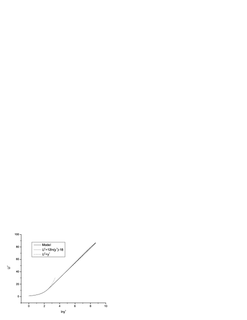
Figure 4: The velocity profile as predicted by the model with $\nu^{+}_{p}=10^{4}$ and Re${}_{\tau}=590$.

We observe that $V^{+}$ is increasing with a constant rate for small $y^{+}$ and then follows the log-law of the MDR. The results for $\lambda=1$ are shown in Fig. 5.

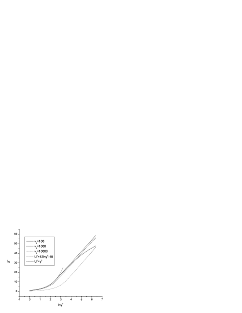
Figure 5: The velocity profile predicted by the model with Re${}_{\tau}=590$ and $\lambda=1$ for various values of $\nu^{+}_{p}$.

We note that for $\nu_{p}=100$ the velocity profile first follows the viscous profile and then joins the MDR until it begins to cross back to the Newtonian plug. For $\nu_{p}$=1000 the viscous layer is increased in size, but then the velocity profile becomes parallel to the MDR but with a smaller intercept, signaling less efficicient drag reduction. Once $\nu_{p}$ reaches the value of 10 000, the viscous layer becomes rather large, of the order of 20. The velocity profile sill succeeds to run parallel the MDR, but with a much reduced intercept.

To compare the prediction of the model to the experimental results shown in Fig. 1 we need to relate Re_τ to Re as used in that figure. The relation is

$${\rm Re}_{L}\equiv Re_{\tau}V^{+}_{L}\ ,$$ (39)

where $V^{+}_{L}$ is the velocity at the center of the channel. Fig. 6 shows $f^{-1/2}$ as a function of $\log_{10}({\rm Re}_{L}f^{1/2})$ with various values of $\nu_{p}$. One can see that for large $\nu_{p}$, we obtain a drag enhancement when Re is small. This enhancement decreases with increasing Re and eventually for large enough Re there is drag reduction. The maximum amount of drag reduction, however, cannot exceed the MDR. For small $\nu_{p}$, the drag enhancement is nearly unnoticeable. However, drag reduction in this case is smaller for large Re because the Newtonian plug occurred earlier. It should be noted that the curves in Fig. 6 exhibit the “ladder” characteristics for different values of $\nu_{p}$. This was identified as “Type B” drag reduction by Virk ASME , and is the fundamental characteristic of drag reduction by rod-like polymers. We see that our results agree reasonably well with the experiments presented in Prandtl-Kármán coordinates.

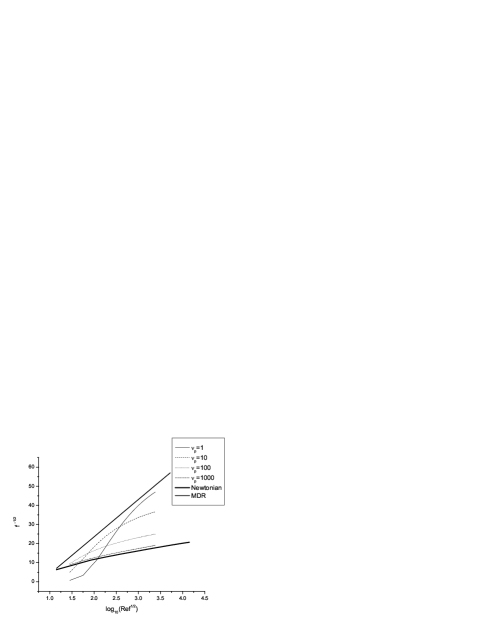
Figure 6: $f^{-1/2}$ as the function of $\log_{10}({\rm Re}f^{1/2})$ with $\lambda=1$ with various values of $\nu_{p}$.

To compare the theory to the experimental results in DR(%) vs Re coordinates we use the experimentally measured values of $g$ and $\nu_{p}$ to predict the amount of drag reduction. As we mentioned before, the effective viscosity in laminar flow of XG solutions is well-approximated by Ostwald-de Waele model. This implies in the low-Re flow, $g$ is given by (in MKS units):

$$g=k_{1}S^{n-1}=k_{1}\left(\frac{\nu_{0}{\rm Re}_{\tau}^{2}}{L^{2}}\right)^{n-1}\ ,$$ (40)

where the last equality is obtained by multiplying Eq. (26) by $\gamma$. The experimental value of $\nu_{p}$ for XG solution is given by (in MKS units):

$$\nu_{p}=0.011147~{}C^{1.422}\nu_{0}\ ,$$ (41)

where $C$ is the concentration of XG in wppm. The value of $f$ can then be calculated by: (i) obtaining the experimental values of $C$, $k_{1}$ and $n$ for Eqs. (40) and (41), (ii) rescaling the variables $S$, $K$ and $W$ by Eq(29) and finally, (iii) solving Eqs. (38) and (32) to get $f$ as a function of ${\rm Re}_{L}$. It should be noted that in the present experiments the definition of Reynolds number is in general different from our definition in (39). For the sake of comparison of the theory with the experiments we assume that two Reynolds numbers are proportional to each other:

$${\rm Re}_{L}=12{\rm Re}_{\rm exp}\ .$$ (42)

Fig. 7 shows the comparison of the percentage of drag reduction (enhancement) between the theoretical predictions and the experimental results. The two data sets shown pertain to $c=250$wppm ($k_{1}=11.04,\ n=0.727$) and $c=500$wppm ($k_{1}=11.04,\ n=0.727$). The agreement between theory and experiment is very satisfactory.

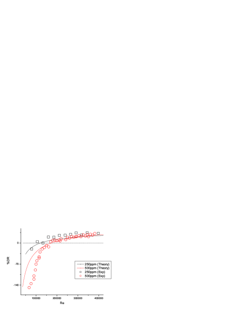
Figure 7: $f^{-1/2}$ as the function of $\log_{10}({\rm Re}f^{1/2})$ with $\lambda=1$ with various values of $\nu_{p}$.

V Discussion and Conclusions

In summary, we studied the Re dependence of the drag reduction by rod-like polymers. We showed that when the value of Re is small, the drag is enhanced due to the homogenous increase of the effective viscosity. When Re is sufficiently large, due to the turbulent activity, the effective viscosity varies as a function of the distance to the wall. As the result, the amount of drag is reduced. We use a simple interpolation between low Re and the high Re flows to account for this. The resulting theoretical results agree semi-quantitatively with the experiments both in Prandtl-Kármán coordinates and in DR(%) vs Re coordinates.

It should be noted that only rod-like polymers exhibit drag enhancement for low Re. For flexible polymers, the drag is the same as that of the Newtonian flow for low Re, and only after a critical value of Re, the drag reduction sets in Virk ; Bonn2 . This difference in behavior from rod-like polymers is because the flexible polymers are coiled when Re is small. They do not affect the flow unless Re increases enough to allow the shear to develop to affect the coil-stretch transition in the flexible polymers. In contrast, rod-like polymers are always extended and therefore they can affect the flow for all Re.

- (1) B. A. Toms, 1st Internat. Congr. Rheol., Amsterdam, 1949, 2, 135.
- (2) P.S. Virk, AIChE 21, 625 (1975).
- (3) A. Gyr and H. W. Bewersdorff Drag Reduction of Turbulent Flows by Additives (Kluwe, London, 1995).
- (4) P. S. Virk, D. L. Wagger and E. Koury, ASME FED- Vol.237, pp. 261.
- (5) C. Wagner, Y. Amarouchène, P. Doyle and D. Bonn, Europhys. Lett. 64, 823 (2003).
- (6) O.Cadot, D.Bonn, S.Douady, Phys. Fluids 10, 426 (1998).
- (7) R.B.Bird, R.C.Armstrong, O.Hassager, Dynamics of Polymeric Liquids vol 1&2 (Wiley, NY, 1987).
- (8) A. Lindner, D. Bonn, E. Corvera Poire, M. Ben Amar, J. Meunier, J. Fluid.Mech, 469, 237 (2002).
- (9) A.V.Bazilevskii, S.I.Voronkov, V.M.Entov, A.N.Rozhkov, Phys. Dokl. 26, 333 (1981); S.L.Anna, G.H.McKinley, J. Rheol. 45, 115 (2000); Y.Amarouchene, D.Bonn, J.Meunier, H.Kellay, Phys. Rev. Lett. 86, 3558 (2001).
- (10) F.T.Trouton, Phil. Mag. 19, 347 (1906).
- (11) M. Doi and S. F. Edwards The Theory of Polymer Dynamics (Oxford, 1988).
- (12) V. S. L’vov, A. Pomyalov, I. Procaccia and V. Tiberkervich, Phys. Rev. Lett., 94, 174502 (2005).
- (13) S.B. Pope, Turbulent Flows (Cambridge, 2000).
- (14) R. Benzi, E. S.C. Ching, T. S. Lo, V. S. L’vov, and I. Procaccia, Phys. Rev. E., 72, 016305(2005).
- (15) R. Benzi, E. deAngelis, V. S. L’vov and I. Procaccia, Phys. Rev. Lett., 95, 194502 (2005).
- (16) V. S. L’vov, A. Pomyalov and V. Tiberkevich, Environ. Fluid Mech., 5, 373, (2005).
- (17) P. S. Virk, AlChE Journal 21, 625 (1975).
- (18) D. Bonn, Y. Amarouchǹe, C. Wagner, S. Douady and O. Cadot, J. Phys.: Condens. Matter, 17, S1195 (2005).