The Painlevé Test and Reducibility to the Canonical Forms

The Painlevé Test and Reducibility
to the Canonical Forms for Higher-Dimensional
Soliton Equations with Variable-Coefficients

Tadashi KOBAYASHI ^† and Kouichi TODA ^‡ T. Kobayashi and K. Toda

^† High-Functional Design G, LSI IP Development Div., ROHM CO., LTD.,
  21, Saiin Mizosaki-cho, Ukyo-ku, Kyoto 615-8585, Japan t-kobayashi@st.pu-toyama.ac.jp

^‡ Department of Mathematical Physics, Toyama Prefectural University,
  Kurokawa 5180, Imizu, Toyama, 939-0398, Japan kouichi@yukawa.kyoto-u.ac.jp

Received November 30, 2005, in final form June 17, 2006; Published online June 30, 2006

The general KdV equation (gKdV) derived by T. Chou is one of the famous $(1+1)$ dimensional soliton equations with variable coefficients. It is well-known that the gKdV equation is integrable. In this paper a higher-dimensional gKdV equation, which is integrable in the sense of the Painlevé test, is presented. A transformation that links this equation to the canonical form of the Calogero–Bogoyavlenskii–Schiff equation is found. Furthermore, the form and similar transformation for the higher-dimensional modified gKdV equation are also obtained.

KdV equation with variable-coefficients; Painlevé test; higher-dimensional integrable systems

37K10; 35Q53

1 Introduction

Modern theories of nonlinear science have been widely developed over the last half-century. In particular, nonlinear integrable systems have attracted much interest among mathematicians and physicists. One of the reasons for this is the algebraic solvability of the integrable systems. Apart from their theoretical importance, they have remarkable applications to many physical systems such as hydrodynamics, nonlinear optics, plasma and field theories and so on [1, 2, 3]. Generally the notion of the nonlinear integrable systems [4] is not defined precisely, but rather is characterized by a number of common features: space-localized solutions (or solitons) [5, 6, 7, 8, 9], Lax pairs [10, 11, 12], bi-Hamiltonians [12, 13], Bäcklund transformations [9, 14] and Painlevé tests [15, 16, 17, 18, 19, 20, 21]. Moreover, solitons and nonlinear evolution equations are a major subject in mechanical and engineering sciences as well as mathematical and physical ones. Among the well-known soliton equations, the celebrated Korteweg–de Vries (KdV) [22] and Kadomtsev-Petviashvili (KP) [23] equations possess remarkable properties. For example, a real ocean is inhomogeneous and the dynamics of nonlinear waves is very influenced by refraction, geometric divergence and so on. The problem of evolution of transverse perturbations of a wave front is of theoretical and practical interest. However, finding new integrable systems is an important but difficult task because of their somewhat ambiguous definition and undeveloped mathematical background.

The physical phenomena in which many nonlinear integrable equations with constant coefficients arise tend to be very highly idealized. Therefore, equations with variable coefficients may provide various models for real physical phenomena, for example, in the propagation of small-amplitude surface waves, which runs on straits or large channels of slowly varying depth and width. On one hand, there has been much interest in the study of generalizations with variable coefficients of nonlinear integrable equations [24, 25, 26, 27, 28, 29, 30, 31, 32, 33, 34, 35, 36, 37, 38, 39, 40, 41, 42, 43, 44, 45].

For discovery of new nonlinear integrable systems, many researchers have mainly investigated ($1+1$)-dimensional nonlinear systems with constant coefficients. On the other hand, there are few research studies to find nonlinear integrable systems with variable coefficients, since they are essentially complicated. And their results are still in its early stages. Analysis of higher-dimensional systems is also an active topic in nonlinear integrable systems. Since then the study of integrable nonlinear equations in higher dimensions with variable coefficients has attracted much more attention. So the purpose of this paper is to construct a ($2+1$) dimensional integrable version of the KdV and modified KdV [46] equations with variable coefficients.

It is widely known that the Painlevé test in the sense of the Weiss–Tabor–Carnevale (WTC) method [16] is a powerful tool for investigating integrable equations with variable coefficients. We have discussed the following higher-dimensional 3rd order nonlinear evolution equation with variable coefficients for $u=u(x,z,t)$ [47, 48]:

$$u_{t}+a(x,z,t)u+b(x,z,t)u_{x}+c(x,z,t)u_{z}+d(x,z,t)uu_{z}+e(x,z,t)u_{x}\partial_{x}^{-1}u_{z}$$

$$\qquad{}+f(x,z,t)u_{xxz}+g(x,z,t)=0,$$ (1)

where $d(x,z,t)+e(x,z,t)\neq 0$, $f(x,z,t)\neq 0$ and subscripts with respect to independent variables denote their partial derivatives, for example, $u_{x}=\partial u/\partial x$, $u_{xz}=\partial^{2}u/\partial x\partial z$ etc, and $\partial_{x}^{-1}u:=\displaystyle\int^{x}u(X)dX$. Here $a(x,z,t),b(x,z,t),\ldots,g(x,z,t)$ are coefficient functions of two spatial variables $x$, $z$ and one temporal variable $t$. We have carried out the WTC method for equation (1), and have presented two sets of the coefficient function so that it is shown in next section. Equations of the form (1) include one of the integrable higher-dimensional KdV equations:

$$u_{t}+uu_{z}+\frac{1}{2}u_{x}\partial_{x}^{-1}u_{z}+\frac{1}{4}u_{xxz}=0,$$ (2)

which is called the Calogero–Bogoyavlenskii–Schiff (CBS) equation [49, 50, 51, 52, 53]. Equation (2) will be the standard KdV equation for $u=u(x,t)$:

$$u_{t}+\frac{3}{2}uu_{x}+\frac{1}{4}u_{xxx}=0$$

by a dimensional reduction $\partial_{z}=\partial_{x}$, and the Ablowitz–Kaup–Newell–Segur (AKNS) equation for $u=u(x,t)$ [54, 55]:

$$u_{t}+uu_{t}+\frac{1}{2}u_{x}\partial_{x}^{-1}u_{t}+\frac{1}{4}u_{xxt}=0$$

by another dimensional reduction $\partial_{z}=\partial_{t}$. Here (and hereafter) $\partial_{x}\equiv\partial/\partial x$, $\partial_{t}\equiv\partial/\partial t$ and so on.

This paper is organized as follows. In Section 2, we will review the process of the WTC method of equation (1) in brief. In Section 3 and 4 we will consider a general KdV and a general modified KdV equations in ($2+1$) dimensions corresponding a special but interesting case of the integrable higher-dimensional KdV equation with variable coefficients given in Section 2. Section 5 will be devoted to conclusions.

2 Painlevé test of equation (1)

Let us now briefly review the process of the Painlevé test in the sense of the WTC method for equation (1) put forward in [47] and then in [48].

Weiss et al. said in [16] that a partial differential equation (PDE) has the Painlevé property when the solutions of the PDE are single-valued around the movable singularity manifold. They have proposed a technique that determines whether or not a given PDE is integrable, which we call the WTC method:

When the singularity manifold is determined by

$$\phi(z_{1},\ldots,z_{n})=0,$$ (3)

and $u=u(z_{1},\ldots,z_{n})$ is a solution of PDE given, then we assume that

$$u=\sum_{j=0}^{\infty}u_{j}\phi^{j-\alpha},$$ (4)

where $\phi=\phi(z_{1},\ldots,z_{n})$, $u_{j}=u_{j}(z_{1},\ldots,z_{n})$, $u_{0}\neq 0$ ($j=0,1,2,\ldots$) are analytic functions of $z_{j}$ in a neighborhood of the manifold (3), and $\alpha$ is a positive integer called the leading order. Substitution of expansion (4) into the PDE determines the value of $\alpha$ and defines the recursion relations for $u_{j}$. When expansion (4) is correct, the PDE possesses the Painlevé property and is conjectured to be integrable.

Now we show the WTC method for equation (1). For that, a nonlocal term of equation (1) should be eliminated. We have a potential form of equation (1) in terms of $U=U(x,z,t)$:

$$U_{xt}+a(x,z,t)U_{x}+b(x,z,t)U_{xx}+c(x,z,t)U_{xz}+d(x,z,t)U_{x}U_{xz}+e(x,z,t)U_{xx}U_{z}$$

$$\qquad{}+f(x,z,t)U_{xxxz}+g(x,z,t)=0,$$ (5)

when defining $u=U_{x}$. We are now looking for a solution of equation (5) in the Laurent series expansion with $\phi=\phi(x,z,t)$:

$$U=\sum^{\infty}_{j=0}U_{j}\phi^{j-\alpha},$$ (6)

where $U_{j}=U_{j}(x,z,t)$ are analytic functions in a neighborhood of $\phi=0$. In this case, the leading order ($\alpha$) is $1$ and

$$U_{0}=12\frac{f(x,z,t)}{d(x,z,t)+e(x,z,t)}\phi_{x}$$

is given. Then, after substituting of the expansion (6) into equation (5), the recursion relations for the $U_{j}$ are presented as follows:

$$(j+1)(j-1)(j-4)(j-6)f(x,z,t)\phi_{x}^{3}\phi_{z}U_{j}=F(U_{j-1},\ldots,U_{0},\phi_{t},\phi_{x},\phi_{z},\ldots),$$

where the explicit dependence on $x$, $z$, $t$ of the right-hand side comes from that of the coefficients. It is found that the resonances occur at

$$j=-1,~{}1,~{}4,~{}6.$$ (7)

Then one can check that the numbers of the resonances (7) correspond to arbitrary functions $\phi$, $U_{1}$, $U_{4}$ and $U_{6}$, though we have omitted the details in this paper. We have succeeded in finding of two forms of the higher-dimensional KdV equation with variable coefficients given by

$$u_{t}+\left\{\frac{d^{\prime}(t)}{d(t)}-\frac{f^{\prime}(t)}{f(t)}+\frac{4}{3}\big{(}\alpha(z,t)-\beta(t)+c_{z}(z,t)\big{)}\right\}u+\frac{2}{3}x\big{(}\alpha(z,t)-\beta(t)+c_{z}(z,t)\big{)}u_{x}$$

$$\qquad{}+c(z,t)u_{z}+d(t)uu_{z}+\frac{d(t)}{2}u_{x}\partial_{x}^{-1}u_{z}+f(t)u_{xxz}+g(z,t)=0,$$ (8)

and

$$u_{t}+\big{(}2A(z,t)-\eta^{\prime}(t)\big{)}u+c(z,t)u_{z}+\big{(}A(z,t)x+B(z,t)\big{)}u_{x}+d(z,t)uu_{z}$$

$$\qquad{}+\frac{d(z,t)}{2}u_{x}\partial_{x}^{-1}u_{z}+\frac{3}{2}d(z,t)\exp{\eta(t)}u_{xxz}+g(z,t)=0.$$ (9)

In this paper, $(\cdot)^{\prime}$ denotes the ordinary derivative with respect to the independent variable. Apparently, equations (8) and (9) are (more general) higher-dimensional integrable versions of the $(1+1)$ dimensional KdV equations with variable coefficients appeared in [24, 25, 26, 27, 28, 29, 30, 31, 32, 33, 38]. It is easy to check by suitable choice of coefficient functions after the dimensional reduction $\partial_{z}=\partial_{x}$.

3 A general KdV equation in $\boldsymbol{(2+1)}$ dimensions

We consider a special but interesting case of equation (8) in this section.

Setting the following condition of variable coefficients:

$$\alpha(z,t)-\beta(t)=\frac{3}{4}\frac{G^{\prime}(t)}{G(t)},\quad c(z,t)=0,\quad d(t)=1,\quad f(t)=\frac{1}{4},\quad g(z,t)=0,$$

equation (8) becomes the following ($2+1$) dimensional equation [56]:

$$u_{t}+uu_{z}+\frac{1}{2}u_{x}\partial_{x}^{-1}u_{z}+\frac{1}{4}u_{xxz}-\frac{G^{\prime}(t)}{G(t)}u-\frac{x}{2}\frac{G^{\prime}(t)}{G(t)}u_{x}=0.$$ (10)

Here $G(t)$ is an arbitrary function of the temporal variable $t$. We would like to call equation (10) a general Calogero–Bogoyavlenskii–Schiff (gCBS) equation. Because equation (10) is a higher-dimensional integrable version of the general KdV (gKdV) equation [28, 38]:

$$u_{t}+\frac{3}{2}uu_{x}+\frac{1}{4}u_{xxx}-\frac{G^{\prime}(t)}{G(t)}u-\frac{x}{2}\frac{G^{\prime}(t)}{G(t)}u_{x}=0.$$ (11)

And using the Lax-pair Generating Technique [48, 57, 58], we obtain a pair of linear operators associated with equation (10) given by

$$L=\frac{1}{G(t)}\bigr{(}\partial_{x}^{2}+u\bigr{)}-\lambda\equiv\frac{1}{G(t)}L_{{\rm GKdV}}-\lambda,$$ (12)

$$T=\partial_{z}L_{{\rm GKdV}}+\frac{1}{2}\biggr{(}\partial_{x}^{-1}u_{z}-x\frac{G^{\prime}(t)}{G(t)}\biggr{)}\partial_{x}-\frac{1}{4}\biggr{(}u_{z}-\frac{G^{\prime}(t)}{G(t)}\biggr{)}+\partial_{t}.$$ (13)

The compatibility condition of the operators $L$ and $T$ is defined as

$$[L,T]\equiv LT-TL=0,$$ (14)

which gives corresponding integrable equations. Notice here that $\lambda=\lambda(z,t)$ is the spectral parameter and satisfies the non-isospectral condition [48, 56, 59, 60]:

$$\lambda_{t}=\lambda\lambda_{z}.$$

Let here mention exact solutions of the gCBS equation (10). As a result of using of the following transformation:

$$\bar{x}=x\sqrt{G(t)},\quad\bar{z}=z,\quad\bar{t}=\partial_{t}^{-1}G(t),\quad\bar{u}(\bar{x},\bar{z},\bar{t})=\frac{u(x,z,t)}{G(t)},$$ (15)

equation (10) becomes the canonical form of the CBS equation (2) in terms of $\bar{u}=\bar{u}(\bar{x},\bar{z},\bar{t})$ [61]:

$$\bar{u}_{\bar{t}}+\bar{u}\bar{u}_{\bar{z}}+\frac{1}{2}\bar{u}_{\bar{x}}\partial_{\bar{x}}^{-1}\bar{u}_{\bar{z}}+\frac{1}{4}\bar{u}_{\bar{x}\bar{x}\bar{z}}=0.$$ (16)

The $N$ line-soliton solutions with $\tau_{N}=\tau_{N}(\bar{x},\bar{z},\bar{t})$ for equation (16) were expressed as

$$\bar{u}=2(\log\tau_{N})_{\bar{x}\bar{x}},$$

$$\tau_{N}=1+\sum^{N}_{n=1}\sum_{{}_{N}C_{n}}A_{i_{1}\cdots i_{n}}\exp(\lambda_{i_{1}}+\cdots+\lambda_{i_{n}}),$$

$$\lambda_{j}=p_{j}\bar{x}+q_{j}\bar{z}+r_{j}\bar{t}+s_{j},\quad j=1,2,\ldots,N,$$

$$r_{j}=-\frac{p_{j}^{2}q_{j}}{4},$$

$$A_{i_{1}\cdots i_{n}}\equiv A_{i_{1},i_{2}}\cdots A_{i_{1},i_{n}}\cdots A_{i_{n-1},i_{n}},$$

$$A_{ij}=\biggr{(}\frac{p_{i}-p_{j}}{p_{i}+p_{j}}\biggr{)}^{2},$$

where the summation ${}_{N}C_{n}$ indicates summation over all possible combinations of $n$ elements taken from $N$, and symbols $s_{j}$ always denote arbitrary constants [52]. So exact solutions of equation (10) can be presented via the transformation (15). We would like to illustrate line-soliton solutions with $G(t)=1/t$. Figs. 1 and 2 are time evolutions of one line-soliton (with $p_{1}$ and $q_{1}$) and two line-soliton (with $p_{1}$, $p_{2}$, $q_{1}$ and $q_{2}$) solutions. And a V-soliton type solution appears on Fig. 3 setting $p_{1}=p_{2}$ in two line-soliton solutions.

A modified equation corresponding to the gCBS equation (10) will be given in next section.

   

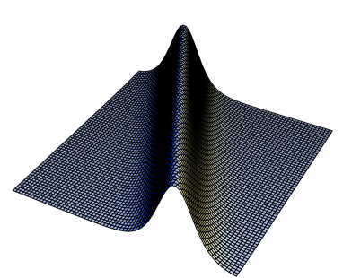
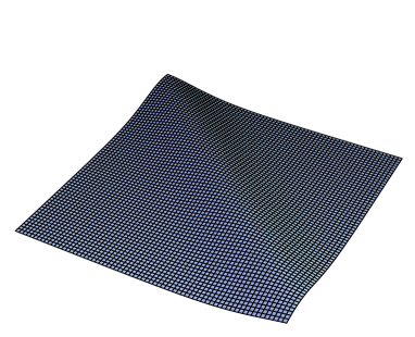
Figure 1: One line-soliton ($t$ = 1 $\to$ $t=5$).

   

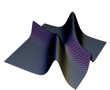
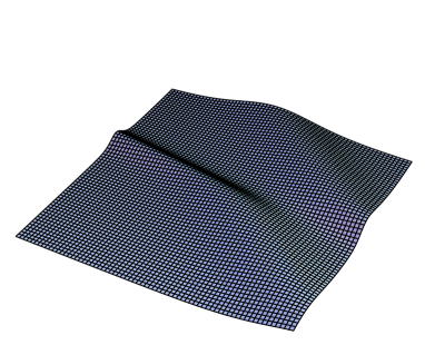
Figure 2: Two line-solitons ($t$ = 1 $\to$ $t=5$).

   

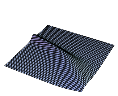
Figure 3: V-soliton ($t$ = 1 $\to$ $t=5$).

4 A modified general KdV equation in $\boldsymbol{(2+1)}$ dimensions

We present a higher-dimensional integrable versions of the modified gKdV (mgKdV) equation [29] from the Lax pair (12) and (13) as follows.

Using the Lax-pair Generating Technique, we obtain a following Lax pair:

$$L=\frac{1}{G(t)}\bigr{(}\partial_{x}^{2}+v\partial_{x}\bigr{)}-\lambda\equiv\frac{1}{G(t)}L_{{\rm GmKdV}}-\lambda,$$

$$T=\partial_{z}L_{{\rm GmKdV}}+\frac{1}{2}\bigr{(}\partial_{x}^{-1}v_{z}\bigr{)}\partial_{x}^{2}+\frac{1}{2}\left(v\partial_{x}^{-1}v_{z}-\frac{1}{4}\partial_{x}^{-1}\bigr{(}v^{2}\bigr{)}_{z}-\frac{1}{2}v_{z}-\frac{G^{\prime}(t)}{G(t)}\right)\partial_{x}+\partial_{t}.$$

Note here that $\lambda$ satisfies a non-isospectral condition:

$$\lambda_{t}=\lambda^{2}\lambda_{z}.$$

Then the Lax equation (14) gives a higher-dimensional mgKdV equation, or a modified gCBS equation for $v=v(x,z,t)$:

$$v_{t}-\frac{1}{4}v^{2}v_{z}-\frac{1}{8}v_{x}\partial_{x}^{-1}\bigr{(}v^{2}\bigr{)}_{z}+\frac{1}{4}v_{xxz}-\frac{1}{2}\frac{G^{\prime}(t)}{G(t)}v-\frac{x}{2}\frac{G^{\prime}(t)}{G(t)}v_{x}=0.$$ (17)

One can also easily check that equation (17) can be reduced to the canonical form of the mgKdV equation for $v=v(x,t)$ [29]:

$$v_{t}-\frac{3}{8}v^{2}v_{x}+\frac{1}{4}v_{xxx}-\frac{1}{2}\frac{G^{\prime}(t)}{G(t)}v-\frac{x}{2}\frac{G^{\prime}(t)}{G(t)}v_{x}=0,$$

by the dimensional reduction $\partial_{z}=\partial_{x}$. Via the transformation as follows:

$$\bar{x}=x\sqrt{G(t)},\quad\bar{z}=z,\quad\bar{t}=\partial_{t}^{-1}G(t),\quad\bar{v}(\bar{x},\bar{z},\bar{t})=\frac{v(x,z,t)}{\sqrt{G(t)}},$$ (18)

equation (17) becomes the modified CBS one for $\bar{v}=\bar{v}(\bar{x},\bar{z},\bar{t})$ [61]:

$$\bar{v}_{\bar{t}}-\frac{1}{4}\bar{v}^{2}\bar{v}_{\bar{z}}-\frac{1}{8}\bar{v}_{\bar{x}}\partial_{\bar{x}}^{-1}\bigr{(}\bar{v}^{2}\bigr{)}_{\bar{z}}+\frac{1}{4}\bar{v}_{\bar{x}\bar{x}\bar{z}}=0,$$ (19)

whose $N$ line-soliton solutions were given similarly in [52].

5 Conclusions

In mechanical, physical, mathematical and engineering sciences, nonlinear systems play an important role, especially those with variable coefficients for certain realistic situations. In this paper we have presented higher-dimensional gKdV and modified gKdV equations (10) and (17), which are integrable in the sense of the Painlevé test. Then we have found the transformations (15) and (18), which link equations (10) and (17) to the canonical forms (16) and (19), respectively. And also $N$ line-soliton solutions to equations (10) and (17) have been given via the transformations (15) and (18), respectively.

By applying the (weak) Painlevé test, we are searching variable-coefficient forms of the nonlinear Schrödinger, sine-Gordon, Camassa–Holm and Degasperis–Procesi equations in ($2+1$) dimensions and so on. Here we would like to give only the form of the ($2+1$) dimensional nonlinear Schrödinger equation for $\phi=\phi(x,z,t)$ [66, 67, 68, 69]:

$$i\phi_{t}+a(x)b(t)\phi_{xz}+b(t)\phi\partial^{-1}_{x}(|\phi|^{2})_{z}+\left\{c(z,t)+\partial_{x}^{-1}\left(\frac{1}{a(x)}\right)\right\}\phi+\frac{1}{2}b(t)a^{\prime}(x)\phi_{z}=0,$$

where $i^{2}=-1$. The detail will be reported in [70]. We will study relations of nonlinear integrable equations with variable coefficients given in this paper to realistic situations in mechanical, physical, mathematical and engineering sciences. Though our program is going well now, there are still many things worth studying to be seen.

Finally let us mention two forms with variable coefficients of the AKNS equation for $u=u(x,t)$:

$$u_{t}+\left\{\frac{d^{\prime}(t)}{d(t)}-\frac{f^{\prime}(t)}{f(t)}+\frac{4}{3}\big{(}\alpha(t)-\beta(t)+c^{\prime}(t)\big{)}\right\}u+\frac{2}{3}x\big{(}\alpha(t)-\beta(t)+c^{\prime}(t)\big{)}u_{x}$$

$$\qquad{}+c(t)u_{t}+d(t)uu_{t}+\frac{d(t)}{2}u_{x}\partial_{x}^{-1}u_{t}+f(t)u_{xxt}+g(t)=0,$$ (20)

and

$$u_{t}+\big{(}2A(t)-\eta^{\prime}(t)\big{)}u+c(t)u_{t}+\big{(}A(t)x+B(t)\big{)}u_{x}+d(t)uu_{t}+\frac{d(t)}{2}u_{x}\partial_{x}^{-1}u_{t}$$

$$\qquad{}+\frac{3}{2}d(t)\exp{\eta(t)}u_{xxt}+g(t)=0,$$ (21)

which are derived from equations (8) and (9) by the dimensional reduction $\partial_{z}=\partial_{t}$. Equations (20) and (21) seem to be new. However it is not certain that equations (20) and (21) are integrable. We are now looking for corresponding transformations into the canonical form of the conventional $(1+1)$ dimensional AKNS equation.

Acknowledgements

Many helpful discussions with Drs. Y. Ishimori, A. Nakamula, T. Tsuchida, S. Tsujimoto, Professors Y. Nakamura and P.G. Estévez are acknowledged. One of the authors (K.T.) would like to thank Professor X.-B. Hu and his graduate students for kind hospitality and useful discussions during his stay at the Chinese Academy of Sciences (Beijing, China) in 2005, where part of this study has been done. The authors wish to extend their thanks to anonymous referees for their helpful and critical comments as this paper took shape.

This work was supported by the First-Bank of Toyama Scholarship Foundation and in part by Grant-in-Aid for Scientific Research (#15740242) from the Ministry of Education, Culture, Sports, Science and Technology.

References

- [1] Lamb Jr.G.L., Elements of soliton theory, New York, Wiley, 1980.
- [2] Akhmediev N.N., Ankiewicz A., Solitons: nonlinear pulses and beams, London, Chapman & Hall, 1997.
- [3] Infeld E., Rowlands G., Nonlinear waves, solitons and chaos, 2nd ed., Cambridge, Cambridge University Press, 2000.
- [4] Zakharov V.E. (Editor), What is integrability?, Berlin, Springer-Verlag, 1991.
- [5] Ablowitz M.J., Segur H., Solitons and the inverse scattering transform, Philadelphia, Society for Industrial & Applied Mathematics, 1981.
- [6] Jeffrey A., Kawahara T., Asymptotic methods of nonlinear wave theory, London, Pitman Advanced Publ., 1982.
- [7] Drazin P.G., Johnson R.S., Solitons: an introduction, Cambridge, Cambridge University Press, 1989.
- [8] Ablowitz M.J., Clarkson P.A., Solitons, nonlinear evolution equations and inverse scattering, Cambridge, Cambridge University Press, 1991.
- [9] Hirota R., The direct methods in soliton theory, Cambridge, Cambridge University Press, 2004.
- [10] Lax P.D., Integrals of nonlinear equations of evolution and solitary waves, Comm. Pure Appl. Math., 1968, V.21, 467–490.
- [11] Calogero F., Degasperis A., Spectral transform and solitons I, Amsterdam, Elsevier Science, 1982.
- [12] Błaszak M., Multi-Hamiltonian theory of dynamical dystems, Berlin, Springer-Verlag, 1998.
- [13] Dickey L.A., Soliton equations and Hamiltonian systems, Singapore, World Scientific, 1990.
- [14] Rogers C., Schief W.K., Bäcklund and Darboux transformations, Cambridge, Cambridge University Press, 2002.
- [15] Ramani A., Dorizzi B., Grammaticos B., Painlevé conjecture revisited, Phys. Rev. Lett., 1982, V.49, 1539–1541.
- [16] Weiss J., Tabor M., Carnevale G., The Painlevé property for partial differential equations, J. Math. Phys., 1983, V.24, 522–526.
- [17] Gibbon J.D., Radmore P., Tabor M., Wood D., Painlevé property and Hirota’s method, Stud. Appl. Math., 1985, V.72, 39–64.
- [18] Steeb W.H., Euler N., Nonlinear evolution equations and Painlevé test, Singapore, World Scientific, 1989.
- [19] Ramani A., Gramaticos B., Bountis T., The Painlevé property and singularity analysis of integrable and non-integrable systems, Phys. Rep., 1989, V.180, 159–245.
- [20] Chowdhury A.R., Painlevé analysis and its applications, New York, Chapman & Hall, 1999.
- [21] Conte R. (Editor), The Painlevé property one century later, New York, Springer-Verlag, 2000.
- [22] Korteweg D.J., de Vries F., On the change of form of long waves advancing in a rectangular canal, and on a new type of long stationary waves, Philos. Mag., 1895, V.39, 422–443.
- [23] Kadomtsev B.B., Petviashvili V.I., On the stability of solitary waves in weakly dispersing media, Dokl. Akad. Nauk SSSR, 1970, V.15, 539–541.
- [24] Calogero F., Degasperis A., Exact solution via the spectral transform of a generalization with linearly -dependent coefficients of the modified Korteweg–de Vries equation, Lett. Nuovo Cimento, 1978, V.22, 270–279.
- [25] Brugarino T., Pantano P., The integration of Burgers and Korteweg–de Vries equations with nonuniformities, Phys. Lett. A, 1980, V.80, 223–224.
- [26] Oevel W., Steeb W.-H., Painlevé analysis for a time-dependent Kadomtsev–Petviashvili equation, Phys. Lett. A, 1984, V.103, 239–242.
- [27] Steeb W.-H., Louw J.A., Parametrically driven sine-Gordon equation and Painlevé test, Phys. Lett. A, 1985, V.113, 61–62.
- [28] Chou T., Symmetries and a hierarchy of the general KdV equation, J. Phys. A: Math. Gen., 1987, V.20, 359–366.
- [29] Chou T., Symmetries and a hierarchy of the general modified KdV equation, J. Phys. A: Math. Gen., 1987, V.20, 367–374.
- [30] Joshi N., Painlevé property of general variable-coefficient versions of the Korteweg–de Vries and non-linear Schrödinger equations, Phys. Lett. A, 1987, V.125, 456–460.
- [31] Hlavatý L., Painlevé analysis of nonautonomous evolution equations, Phys. Lett. A, 1988, V.128, 335–338.
- [32] Brugarino T., Painlevé property, auto-Bäcklund transformation, Lax pairs, and reduction to the standard form for the Korteweg–de Vries equation with nonuniformities, J. Math. Phys., 1989, V.30, 1013–1015.
- [33] Chan W.L., Li K.S., Non-propagating solitons of the non-isospectral and variable coefficient modified KdV equation, J. Phys., 1989, V.27, 883–902.
- [34] Brugarino T., Greco A.M., Painlevé analysis and reducibility to the canonical form for the generalized Kadomtsev–Petviashvili equation, J. Math. Phys., 1991, V.32, 69–72.
- [35] Klimek M., Conservation laws for a class of nonlinear equations with variable coefficients on discrete and noncommutative spaces, J. Math. Phys., 2002, V.43, 3610–3635, math-ph/0011030.
- [36] Gao Y.-T., Tian B., On a variable-coefficient modified KP equation and a generalized variable-coefficient KP equation with computerized symbolic computation, Internat. J. Modern Phys. C, 2001, V.12, 819–833.
- [37] Gao Y.-T., Tian B., Variable-coefficient balancing-act algorithm extended to a variable-coefficient MKP model for the rotating fluids, Internat. J. Modern Phys. C, 2001, V.12, 1383–1389.
- [38] Wang M., Wang Y., Zhou Y., An auto-Bäcklund transformation and exact solutions to a generalized KdV equation with variable coefficients and their applications, Phys. Lett. A, 2002, V.303, 45–61.
- [39] Cascaval R.C., Variable coefficient Korteveg–de Vries equations and wave propagation in elastic tubes, in Evolution Equations, Lecture Notes in Pure and Appl. Math., Vol. 234, New York, Dekker, 2003, 57–69.
- [40] Blanchet A., Dolbeault J., Monneau R., On the one-dimensional parabolic obstacle problem with variable coefficients, in Elliptic and Parabolic Problems, Progr. Nonlinear Differential Equations Appl., Vol. 63, Basel, Birkhauser, 2005, 59–66, math.AP/0410330.
- [41] Fokas A.S., Boundary value problems for linear PDEs with variable coefficients, Proc. R. Soc. Lond. Ser. A Math. Phys. Eng. Sci., 2004, V.460, N 2044, 1131–1151, math.AP/0412029.
- [42] Kobayashi T., Toda K., Extensions of nonautonomous nonlinear integrable systems to higher dimensions, in Proceedings of 2004 International Symposium on Nonlinear Theory and its Applications, 2004, V.1, 279–282.
- [43] Robbiano L., Zuily C., Strichartz estimates for Schrödinger equations with variable coefficients, Mem. Soc. Math. Fr. (N.S.), 2005, N 101–102, math.AP/0501319.
- [44] Loutsenko I., The variable coefficient Hele–Shaw problem, integrability and quadrature identities, math-ph/0510070.
- [45] Senthilvelan M., Torrisi M., Valenti A., Equivalence transformations and differential invariants of a generalized nonlinear Schrödinger equation, nlin.SI/0510065.
- [46] Miura R.M., Gardner C.S., Kruskal M.D., Korteweg–de Vries equation and generalizations. II. Existence of conservation laws and constants of motion, J. Math. Phys., 1968, V.9, 1204–1209.
- [47] Kobayashi T., Toda K., Nonlinear integrable equations with variable coefficients from Painlevé test and their exact solutions, in Proceedings of the 10th International Conference “Modern Group Analysis” (2004, Larnaca, Cyprus), 2005, 214–221.
- [48] Kobayashi T., Toda K., A generalized KdV-family with variable coefficients in () dimensions, IEICE Transactions on Fundamentals of Electronics, Communications and Computer Sciences, 2005, V.E88-A, 2548–2553.
- [49] Calogero F., A method to generate solvable nonlinear evolution equations, Lett. Nuovo Cim., 1975, V.14, 443–447.
- [50] Bogoyavlenskii O.I., Overturning solitons in new two-dimensional integrable equations, Math. USSR-Izv., 1990, V.34, 245–259.
- [51] Schiff J., Integrability of Chern–Simons–Higgs vortex equations and a reduction of the selfdual Yang–Mills equations to three-dimensions, NATO ASI Ser. B, Vol. 278, New York, Plenum, 1992.
- [52] Yu S.-J., Toda K., Sasa N., Fukuyama T., soliton solutions to the Bogoyavlenskii–Schiff equation and a quest for the soliton solution in dimensions, J. Phys. A: Math. Gen., 1998, V.31, 3337–3347.
- [53] Toda K., Yu S.-J., Fukuyama T., The Bogoyavlenskii–Schiff hierarchy and integrable equations in () dimensions, Rep. Math. Phys., 1999, V.44, 247–254.
- [54] Ablowitz M.J., Kaup D.J., Newell A.C., Segur H., The inverse scattering transform-Fourier analysis for nonlinear problems, Stud. Appl. Math., 1974, V.53, 249–315.
- [55] Clarkson P.A., Mansfield E.L., On a shallow water wave equation, Nonlinearity, 1994, V.7, 975–1000, solv-int/9401003.
- [56] Clarkson P.A., Gordoa P.R., Pickering A., Multicomponent equations associated to non-isospectral scattering problems, Inverse Problems, 1997, V.13, 1463–1476.
- [57] Yu S.-J., Toda K., Lax pairs, Painlevé properties and exact solutions of the Calogero–Korteweg–de Vries equation and a new -dimensional equation, J. Nonlinear Math. Phys., 2000, V.7, 1–13, math.AP/0001188.
- [58] Toda K., Extensions of soliton equations to non-commutative dimensions, in JHEP Proceedings of Workshop on Integrable Theories, Solitons and Duality, PR-HEP, 2003, unesp2002/038, 10 pages.
- [59] Gordoa P.R., Pickering A., Nonisospectral scattering problems: a key to integrable hierarchies, J. Math. Phys., 1999, V.40, 5749–5786.
- [60] Estévez P.G., A nonisospectral problem in dimensions derived from KP, Inverse Problems, 2001, V.17, 1043–1052.
- [61] Bogoyavlenskii O.I., Breaking solitons. III, Math. USSR-Izv., 1991, V.36, 129–137.
- [62] Gilson C., Pickering A., Factorization and Painlevé analysis of a class of nonlinear third-order partial differential equations, J. Phys. A: Math. Gen., 1995, V.28, 2871–2888.
- [63] Hone A.N.W., Painlevé tests, singularity structure and integrability, Report UKC/IMS/03/33, IMS, University of Kent, UK, 2003, nlin.SI/0502017.
- [64] Estévez P.G., Prada J., Hodograph transformations for a Camassa–Holm hierarchy in () dimensions, J. Phys. A: Math. Gen., 2005, V.38, 1287–1297, nlin.SI/0412019.
- [65] Gordoa P.R., Pickering A., Senthilvelan M., A note on the Painlevé analysis of a dimensional Camassa–Holm equation, Chaos Solitons Fractals, 2006, V.28, 1281–1284, nlin.SI/0511025.
- [66] Strachan I.A.B., A new family of integrable models in dimensions associated with Hermitian symmetric spaces, J. Math. Phys., 1992, V.33, 2477–2482.
- [67] Strachan I.A.B., Some integrable hierarchies in dimensions and their twistor description, J. Math. Phys., 1993, V.34, 243–259.
- [68] Jiang Z., Bullough R.K., Integrability and a new breed of solitons of an NLS type equation in dimensions, Phys. Lett. A, 1994, V.190, 249–254.
- [69] Kakei S., Ikeda T., Takasaki K., Hierarchy of -dimensional nonlinear Schrödinger equation, self-dual Yang–Mills equation, and toroidal Lie algebras, Ann. Henri Poincaré, 2002, V.190, 817–845, nlin.SI/0107065.
- [70] Kobayashi T., Toda K., Extensions of nonautonomous nonlinear integrable systems to higher dimensions, in preparation.