Self-similarity in Laplacian Growth

Abstract

We consider Laplacian Growth of self-similar domains in different geometries. Self-similarity determines the analytic structure of the Schwarz function of the moving boundary. The knowledge of this analytic structure allows us to derive the integral equation for the conformal map. It is shown that solutions to the integral equation obey also a second order differential equation which is the one dimensional Schroedinger equation with the $\mbox{sinh}^{-2}$-potential. The solutions, which are expressed through the Gauss hypergeometric function, characterize the geometry of self-similar patterns in a wedge. We also find the potential for the Coulomb gas representation of the self-similar Laplacian growth in a wedge and calculate the corresponding free energy.

I Introduction

The Laplacian Growth (LG) phenomena has been studied for a long time in various physical systems ranging from solidification to bacterial colony growth Howison . Displacement of viscous fluid by an invicsid one (to be referred as oil and air) between two closely spaced horizontal plates (the Hele-Shaw cell) is the simplest process of this kind. The Laplacian Growth is defined here as the dynamics of the oil/air interface (Fig. 1a). For a review, see, e.g., RMP ; book .

The process is unstable and produces in a long time an asymptotical shape which is either a finger ST ; TRHC (in channel and wedge geometries) or a fractal with the same universal characteristics HLS-DLA as in diffusion-limited aggregation WittenSanderPRL ; PhTod (in all geometries).

It has been recently discovered that the Laplacian Growth is

• described by the 2D Toda integrable hierarchy MWZ ,

• equivalent to the evolution of the support of eigenvalues in certain ensembles of random matrices MWZ ; KKMWZ ,

• relevant to the 2D fermions in the magnetic field ABWZ , and

• equivalent to Whitham equations of the soliton theory KMWZ .

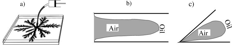
Figure 1: Laplacian Growth in a Hele-Shaw cell for the radial a), channel b), and wedge c) geometries.

The most well studied geometry is a rectangular Hele-Shaw cell (Fig. 1b) where air enters the channel from the left side. The boundary dynamics in this system was considered first by Saffman and Taylor in 1958 ST . They observed a relatively stable finger (known today as the Saffman-Taylor finger) formed after a competition of many fingers generated by an interfacial instability. They also found a continuous family of traveling wave solutions (in the absence of surface tension) and posed a problem of selection of a proper member of the family to describe the observable finger. (See the development of the selection problem in Asympt -M98 ). In the radial geometry (Fig. 1a) an asymptotic shape is a fractal with nontrivial universal self-similar features HLS-DLA , which are still not explained. Another geometry which has been studied both theoretically and experimentally is the wedge geometry (Fig. 1c). In this setting air enters the wedge filled with oil through the wedge corner and pushes oil outward. A number of exact solutions were found in this geometry by different methods TRHC ,Benamar -MV . Some of them are analogs of “traveling wave” solutions. They are also called fingers.

The latter experimental setting is of the great interest for several reasons. One of them is that traveling wave solutions in a wedge geometry are the only known explicit solutions of LG described by conformal maps (from the unit circle), which derivatives contain non-integer singularities. Moreover, they have a very important property of being self-similar.

It is the latter property that we are going to study in detail in this paper. We prove that the only smooth self-similar solution in the radial geometry is an ellipse. The family of self-similar solutions with a singularity at the origin is much more interesting. We show that the exact solutions in the wedge geometry first obtained in Benamar belong to this class.

To study self-similar solutions of general type, we develop a new method which allows us to represent the results for the wedge geometry in a more explicit and transparent form. We will show that the self-similarity completely determines the analytical structure of the Schwarz function of the moving boundary. Using the knowledge of the analytical structure we will derive an integral equation for the conformal map from the exterior of the unit circle to the domain filled by oil. We will establish then the equivalence of this integral equation to the Schrodinger equation with a well-studied (Poeschle-Teller) potential Flugge which was derived for LG in wedge earlier Benamar ; Tu . We will also calculate the free energy of the 2D Coulomb gas representation of LG for the case of self-similar solutions in a wedge.

The paper is organized as follows. In Section II, we introduce the notion of the Schwarz function of a curve. In Section III, we formulate the Laplacian Growth in terms of the Schwarz function of the moving boundary. Section IV treats the property of self-similarity in terms of the Schwarz-function. Sections V and VI are devoted to the self-similar solutions in the wedge. They contain geometric interpretation, derivation of both integral and differential equations for these solutions, proof of their equivalence, and the analytic continuation of the solutions. In section VII, we present the 2D Coulomb gas representation of the self-similar solution and, finally, in section VIII we investigate different limits and special cases which are of particular interest for physics.

II Schwarz Function

The Schwarz function Davis plays a very important role in what follows, so we devote some space here to introduce this object. Let a curve ${\cal C}$ in the plane be given by an equation

$$F(x,y)=0,$$ (1)

where $x$ and $y$ are cartesian coordinates in the plane. Replacing them by complex coordinates $z=x+iy$, $\bar{z}=x-iy$, we rewrite the equation for the curve in the form

$$G(z,\bar{z})=F\left(\frac{z+\bar{z}}{2},\frac{z-\bar{z}}{2i}\right)=0$$ (2)

Solving this equation with respect to $\bar{z}$ (always possible locally for analytic curves) we find

$$\bar{z}=S(z)$$ (3)

The so defined function $S(z)$ is called the Schwarz function of the curve ${\cal C}$. The equation (3) is complex and thus contains two real equations, which are mutually dependent, since each of them bears the same information as the Eq. (1). The constraint on $S$ is clear after taking the conjugate of equation (3):

$$z=\bar{S}(S(z)).$$ (4)

This property of the Schwarz function is called unitarity MWZ . The Schwarz function is holomorphic and has a great advantage over a conformal map description of curves, as it does not imply any particular parametrization on the curve.

The geometrical meaning of the Schwarz function becomes clear if one imagines that the curve ${\cal C}$ is a mirror. Then for the object at a point $z$ close enough to the mirror the image is at the point $\overline{S(z)}$. For instance, the Schwarz function for a circle centered at the origin is $S(z)=R^{2}/z$, where $R$ is the radius of the circle.

Given the Schwarz function $T(w)$ of a closed curve ${\cal T}$ in the (“mathematical”) plane $w$ and the conformal map $f(w)$ from the outside/inside of that curve onto the outside/inside of a curve ${\cal C}$ on the (“physical”) plane $z$, one can easily find the Schwarz function of the curve ${\cal C}$: $S(z)=\bar{f}(T(f^{-1}(z)))$, where $f^{-1}$ denotes the inverse function, and we adopt the standard notation $\bar{f}(z)=\overline{f(\bar{z})}$. In particular, if the curve ${\cal T}$ in the mathematical plane is the unit circle, we find that the Schwarz function is given by

$$S(z)=\bar{f}(1/w),\quad\quad z=f(w)$$ (5)

III Laplacian Growth and the Schwarz function

In this section we formulate the Laplacian Growth in terms of the Schwarz function of the boundary following Howison91 .

For a quasistatic motion of a viscous fluid between two closely spaced parallel surfaces, the Navier-Stokes equation is reduced to the Darcy’s Law Lamb which states that the 2D velocity $\bf{v}$ of the fluid is proportional to the gradient of pressure $p$. In properly rescaled variables it has the form

$${\bf v}=-{\bf\nabla}p$$ (6)

$$\Delta p=0$$ (7)

where the last equation (7) follows from the incompressibility condition $\mbox{div}\,\bf{v}=0$. In the air (zero viscosity) domain pressure is constant, $p=\mbox{const}$. Neglecting surface tension, one concludes that $p(x,y)$ is a harmonic function in the oil domain constant along the boundary. In this paper we consider only a single sink placed at infinity. In this case pressure $p$ behaves at infinity as

$$p(x,y)\simeq-\frac{Q}{2\pi}\log R,\quad R\to\infty,$$ (8)

where $R^{2}=x^{2}+y^{2}$ and $Q$ is the pumping rate (that is the decrease of the oil area per unit time).

Introducing the holomorphic complex potential $W(z)=-p+i\psi$ and the complex velocity $v=v_{x}+iv_{y}$, one can rewrite equation (6) in the form $v=\overline{\partial_{z}W}$. In the case of a single air bubble in the cell the complex potential is given by

$$W(z,t)=\frac{Q}{2\pi}\log w(z,t)$$ (9)

Here $w(z,t)$ is (time dependent) conformal map from the oil domain onto the exterior of the unit circle normalized in such a way that $w(z,t)\simeq z/r(t)$ as $|z|\to\infty$ with a real positive coefficient $r(t)$. This coefficient is called the (external) conformal radius of the air domain. In what follows we set $Q=\pi$. In these units, area of the growing domain is equal to $\pi t$.

Let us describe the oil/air interface by its time-dependent Schwarz function $S(z,t)$. If at time $t$ a point $z$ is at the boundary, $\bar{z}=S(z)$, then at time $t+dt$ the point $z+vdt$ belongs to the new boundary, i.e., $\overline{z+vdt}=S(z+vdt,t+dt)$. Therefore, on the boundary it holds

$$\bar{v}=\dot{S}+S^{\prime}v,$$ (10)

where dot and prime denote partial derivatives with respect to $t$ and $z$.

The unit tangent vector to the boundary equals to $dz/dl$, where $l$ is the arclength $dl=\sqrt{dzd\bar{z}}=dz\sqrt{S^{\prime}}$, so

$$dz/dl=\frac{1}{\sqrt{S^{\prime}}}$$ (11)

In the case of zero surface tension pressure is constant along the boundary, and so its gradient is orthogonal to it. In the complex notation we have

$$\mbox{Re}\frac{\bar{v}}{\sqrt{S^{\prime}}}=0.$$ (12)

From unitarity (4) we find $S^{\prime}=1/\bar{S^{\prime}}$. Together with the previous equation this gives

$$\bar{v}+vS^{\prime}=0.$$ (13)

Using equation (10) and (9) (with $Q=\pi$) we then find

$$\dot{S}=2\bar{v}=2\partial_{z}W=\partial_{z}\log w$$ (14)

After analytical continuation from the boundary, this equation is valid everywhere in the oil domain. Equation (14) connects the change on the Schwarz function of the boundary with the solution to the Dirichlet boundary value problem for the oil domain with given sources/sinks.

One can represent the Schwarz function in the form

$$S(z)=S_{-}(z)+S_{+}(z)$$ (15)

where $S_{-}$ is regular in the oil domain, and $S_{+}$ is regular in the air domain. The function $S_{+}(z)$ is given by the Cauchy integral

$$S_{+}(z,t)=\frac{1}{2\pi i}\oint_{\partial{\sf D}(t)}\frac{\bar{z}^{\prime}dz^{\prime}}{z^{\prime}-z}$$ (16)

where ${\sf D}$ is the air domain and the point $z$ is assumed to be inside it. (A similar Cauchy integral, with the point $z$ outside ${\sf D}$, can be written for $S_{-}$.) As the function $\partial_{z}W$ has no singularities in the oil domain, we find

$$\dot{S}_{+}(z)=0$$ (17)

From this we conclude that all harmonic moments of the oil domain

$$t_{k}=\frac{1}{2\pi ik}\oint_{\partial{\sf D}}\bar{z}z^{-k}dz\frac{1}{2\pi ik}\oint_{\partial{\sf D}}S_{+}(z)z^{-k}dz,\quad k\geq 1,$$ (18)

are integrals of motion. This fact was observed by S.Richardson Richardson .

IV Self-similar solutions. General relations

Self-similarity expresses the fact that the evolution of the domain is just a dilatation of its shape. It means that if initially the Schwarz function of the boundary is $S(z)$, then at any other time $\bar{z}/r(t)=S(z/r(t))$ for the points on the boundary, where the real dilatation parameter, $r(t)$, initially equals to $1$. In other words,

$$S(z,t)=r(t)S(z/r(t)).$$ (19)

Let us take $r(t)$ to be the conformal radius of the growing (air) domain. It is defined as the derivative at infinity of the conformal mapping from the exterior of the unit circle onto the oil domain normalized by the conditions that infinity is sent to infinity and $r(t)>0$. Then $S(z)$ is the Schwarz function of the oil domain scaled so that its conformal radius is $1$.

The self-similar reduction of eq.(14) reads

$$S(z)-zS^{\prime}(z)=2A\,\partial_{z}\log w(z)$$ (20)

where $r^{2}(t)=t/A$ and $w(z)$ is the conformal map of the domain with conformal radius $1$. Taking the contour integral of equation (20) over the boundary we find that the constant $A$ is the area (divided by $\pi$) of the domain with conformal radius $1$.

Since the r.h.s. of (20) is an analytic function in the exterior of ${\sf D}$, this equation implies the relation

$$S_{+}(z)-zS_{+}^{\prime}(z)=0$$

with the general solution

$$S_{+}(z)=sz$$ (21)

where $s$ is a constant. This solution corresponds to an ellipse with the axes ratio $(1+s)/(1-s)$. We thus see that regular self-similar solutions are exhausted by ellipses.

This result is not surprising and can be seen right from equations (17) and (18). Under the dilatations $z\rightarrow rz$ the $k$th harmonic moment changes as $t_{k}\rightarrow t_{k}r^{2-k}$. On the other hand, the harmonic moments are integrals of motion and as such cannot change. This leaves as with the only possibility to have all the moments equal to $0$ except $t_{2}$, which is exactly the statement (21).

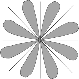
Figure 2: A singular self-crossing domain. The thick lines are the branch cuts of the function $S_{+}$. Spacings between two adjacent fingers are called fjords.

However, there is a family of singular self-similar solutions of equation (20) for which the interface may cross itself at the origin, see Fig. 2 (to be prepared for the next section, the domain looks like $\mbox{$\mathbb{Z}$}_{N}$-symmetric one but in general no additional symmetry is implied). For such solutions the constant $s$ in (21) is different in different sectors of the plane and, therefore, $S_{+}$ has jumps across some rays with $\mbox{arg}\,z=\mbox{const}$ starting at $0$ and coming to $\infty$. We stress that these rays are singularities of $S_{+}$, so they do not depend on $t$. Let $\mit\Gamma$ be such a ray. Take the jump of the both sides of eq. (20) on this ray. Since the r.h.s. is regular, we get

$$[S(z)]_{\mit\Gamma}-z[S^{\prime}(z)]_{\mit\Gamma}=0\,,\quad z\in\mit\Gamma$$

(the jump is defined as $[S(z)]_{\mit\Gamma}=S(ze^{+i0})-S(ze^{-i0})$, $z\in\mit\Gamma$), hence

$$[S(z)]_{\mit\Gamma}=c(\mit\Gamma)\,z\,,\quad z\in\mit\Gamma$$

The jump of $S(z)$ on the branch cut is related to the geometry of the interface around the origin. Let us choose coordinates so that the branch cut is along the positive real semi-axis. Consider a vicinity of the point $z=0$. The function $S^{\prime}(z)$ has a constant jump on the positive part of the real axis equal to $c=c(\mit\Gamma)$. On the other hand, we know that the unit tangent vector to the boundary curve is (11) $l(z)=1/\sqrt{S^{\prime}(z)}$, so using the notation in Fig. 3, we write $l_{1}^{-2}=e^{-2i\theta_{1}}=S^{\prime}(0_{+})$, $l_{2}^{-2}=e^{-2i(\pi-\theta_{2})}=S^{\prime}(0_{-})$ (here $0_{\pm}$ means $\epsilon e^{\pm i0}$ as $\epsilon\to 0$) and so the jump is

$$c=S^{\prime}(0_{+})-S^{\prime}(0_{-})=e^{-2i\theta_{1}}-e^{2i\theta_{2}}$$

Introducing $\theta=\theta_{1}+\theta_{2}$ (the fjord angle) and $\phi=\theta_{1}-\theta_{2}$, we obtain the desired relation

$$c=-2ie^{-i\phi}\sin\,\theta$$ (22)

We see that if $c$ is purely imaginary, then the fjord is symmetric ($\phi=0$) with respect to the real axis.

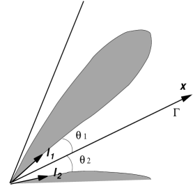
Figure 3: The jump of the Schwarz function is related to the fjord angle.

The connection between the jump of $S_{+}$ and the fjord angle can be understood purely geometrically. Let us consider a symmetric fjord, i.e., the ray $\mit\Gamma$ is the symmetry axis. Very close to the origin the boundaries are almost straight lines. Let us consider a point $ze^{+i0}$, where $z$ is on $\mit\Gamma$. Its reflection in the boundary lies at $ze^{i\theta}=\overline{S(ze^{+i0})}$. For the point $ze^{-i0}$ we have $ze^{-i\theta}=\overline{S(ze^{-i0})}$, so

$$[S(z)]=S(ze^{+i0})-S(ze^{-i0})=(e^{-i\theta}-e^{i\theta})z=cz,$$

from which equation (22) follows.

Using the representation of the Schwarz function via conformal map (5), equation (20) can be rewritten in the familiar form

$$\bar{f}(w^{-1})\partial_{w}f(w)-f(w)\partial_{w}\bar{f}(w^{-1})=\frac{2A}{w}.$$ (23)

The constant $A$ can now be expressed as

$$A=\frac{1}{2\pi i}\oint_{|w|=1}\bar{f}(w^{-1})df(w).$$ (24)

We note that equation (23) looks as the Wronskian of $f(w)$ and $\bar{f}(w^{-1})$. This fact suggests that they are two linearly independent solutions of a second order differential equation of the form

$$w^{2}f^{\prime\prime}(w)+wf^{\prime}(w)+V(w)f(w)=0$$

with a real “potential” $V$, such that $V(w)=\bar{V}(w^{-1})$. Below we shall see that this is indeed the case.

V Symmetric self-similar solutions and solutions in the wedge

In this section, we study a family of self-similar solutions with the $\mbox{$\mathbb{Z}$}_{N}$-symmetry (Fig. 2). Equivalently, these are self-similar solutions in the wedge with the angle $\theta_{0}=2\pi/N$.

Let $\omega=e^{2\pi i/N}$ be the primitive root of unity of degree $N$. The $\mbox{$\mathbb{Z}$}_{N}$-symmetry means that if $z\in{\sf D}$, then $\omega z\in{\sf D}$. For the conformal map this mean that $f(\omega w)=\omega f(w)$ and for the Schwarz function that $S(\omega z)=\omega^{-1}S(z)$. Moreover, from the integral representation (16) we see that the latter property holds for $S_{+}$ and $S_{-}$ separately.

We need to introduce the following notation: Let $\mit\Sigma_{k}$ be the sector $\frac{2\pi}{N}(k-1)\leq\mbox{arg}\,z\leq\frac{2\pi}{N}k$ and let $\mit\Gamma_{k}=\mit\Sigma_{k+1}\cap\mit\Sigma_{k}$ be the ray $\mbox{arg}\,z=\frac{2\pi}{N}k$, see Fig. 4.

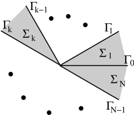
Figure 4: Thick lines $\Gamma_{k}$ are the branch cuts in $S_{+}$. Enumeration of sectors $\Sigma_{k}$ is also shown.

V.1 The integral equation

Combining self-similarity ($S_{+}(z)=s_{k}z$ if $z\in\mit\Sigma_{k}$) with $\mbox{$\mathbb{Z}$}_{N}$-symmetry ($S_{+}(\omega z)=\omega^{-1}S_{+}(z)$) we find that $s_{k+1}=\omega^{-2}s_{k}$ and so

$$s_{k}=\omega^{-2k}s_{0}$$ (25)

Therefore,

$$[S(z)]_{\mit\Gamma_{k}}=c\omega^{-2k}z\,,\quad z\in\mit\Gamma_{k}$$ (26)

where we have set $c=(\omega^{-2}-1)s_{0}$. These jumps are singularities of $S_{+}$.

The definition of the Schwarz function written in the form

$$\bar{f}(w)=S(f(w^{-1}))$$ (27)

implies that singularities of $\bar{f}(w)$ inside the unit circle exactly correspond to singularities of $S(z)$ outside the domain ${\sf D}$, i.e., to singularities of $S_{+}(z)$. In our case $\bar{f}(w)=f(w)$ due to the reflection symmetry with respect to the real axis, and singularities of $f(w)$ are jumps on $N$ intervals $\mbox{arg}\,w=\frac{2\pi}{N}k$, $0<|w|<1$ inside the unit circle, which we denote by $\gamma_{k}$. Therefore, we can write $f(w)$ as the Cauchy type integral

$$f(w)=w+\frac{1}{2\pi i}\sum_{k=0}^{N-1}\int_{0}^{\omega^{k}}\frac{[f(v)]_{\gamma_{k}}dv}{v-w}$$ (28)

(the integral is over $\gamma_{k}$). From (27) we conclude that

$$\left.\phantom{A/B}[f(w)]_{\gamma_{k}}=-\,[S_{+}(z)]_{\mit\Gamma_{N-k}}\right|_{z=f(w^{-1})}=-c\omega^{-2k}f(w^{-1})$$ (29)

(The minus sign is due to the interchange of the two sides of the branch cut when one inverts $w$ .) Plugging this into (28), one obtains, after some transformations:

$$f(w)=w-\frac{c}{2\pi i}\sum_{k=0}^{N-1}\omega^{-2k}\int_{1}^{\infty}\frac{f(\omega^{k}x)\,dx}{(1-\omega^{k}xw)x}$$

Since $f(\omega^{k}x)=\omega^{k}f(x)$, the sum is $\sum_{k}\omega^{-k}/(1-\omega^{k}xw)$ which is easily calculated to be $Nxw/(1-x^{N}w^{N})$, and so we obtain the integral equation for the conformal map:

$$f(w)=w-\frac{cN}{2\pi i}\int_{1}^{\infty}\frac{wf(x)\,dx}{1-w^{N}x^{N}}$$ (30)

with the “boundary condition” $f(1)=0$. Let us denote the fjord angle by $\theta=\pi\beta$, then $c=-2i\sin\,\pi\beta$ (from eq. (22)) and the integral equation acquires the form

$$f(w)=w\,+\,\frac{N\sin\,\pi\beta}{\pi}\int_{1}^{\infty}\frac{wf(v)\,dv}{1-w^{N}v^{N}}\,,\quad\quad f(1)=0$$ (31)

Without using eq. (22), one can find the coefficient in front of the integral by noting that the fjord angle $\pi\beta$ implies that $f(w)\simeq(w-1)^{\beta}$ near the point $w=1$. Expanding eq. (30) around this point, one obtains $c=-2i\sin\,\pi\beta$.

V.2 Geometrical interpretation

There is another way to obtain the Equation (30), namely, from the geometrical arguments applied to multi-logarithmic solutions of 2D LG MS .

We start from a simple observation that each logarithm in the standard multi-logarithmic solution (anzats) for the conformal map of the LG process asymptotically describes a single “U” shaped fjord, a fjord with parallel walls. Let us consider such an anzats:

$$f(w)=rw+\sum_{k}\alpha_{k}\log\left(1-a_{k}/w\right)$$ (32)

where $\alpha_{k}$’s are constants of motion, while all $a_{k}$ ($|a_{k}|<1$) and $r$ are functions of time. Asymptotically at large time $r\rightarrow\infty$ and $|a_{k}|\rightarrow 1$. Integrals of motion for such a solution are

$$\beta_{k}=f(1/\bar{a}_{k})=r/\bar{a}_{k}+\sum_{k^{\prime}}\alpha_{k^{\prime}}\log\left(1-a_{k^{\prime}}\bar{a}_{k}\right)$$ (33)

At large time, when all $a_{k}$s are close to $1$, we can neglect all logarithms except one. Imagine for simplicity that $a_{0}$ is real and $a_{0}\rightarrow 1$, then we can write

$$\beta_{0}\approx r/a_{0}+\alpha_{0}\log(1-a_{0}^{2})\approx r+\alpha_{0}\log(1-a_{0})+\alpha_{0}\log 2,$$ (34)

$$f(1)\approx r+\alpha_{0}\log(1-a_{0})=\beta_{0}-\alpha_{0}\log 2.$$ (35)

This means that asymptotically the bottom of the fjord is at the point $\beta_{0}-\alpha_{0}\log 2$.

Let us now take a number $\delta$ such that $\delta\ll 1$ and $\delta\gg 1-a_{0}$, then using $e^{i\delta}\approx 1+i\delta$ we can calculate

$$f(1+i\delta)\approx r+\alpha_{0}\log(i\delta),$$

$$f(1+i\delta)-f(1-i\delta)=i\pi\alpha_{0}.$$

This shows that the width of the fjord is constant and equals $\pi|\alpha_{0}|$. The direction of the fjord is given by the phase of $\alpha_{0}$.

Using this simple correspondence between the logarithmic singularities and the “U” shape fjords we can construct a so-called “V” shape fjord, i.e., a fjord which walls form a constant angle between them.

It is clear that for this construction we need to put many identical fjords in such a way that they have equal distance between their vertices). All fjord vertices must be on a ray which direction is the same as the direction of the fjord. For the $\mbox{$\mathbb{Z}$}_{N}$-symmetric case we then write:

$$f(w)=rw+\sum_{l=0}^{\infty}\sum_{k=0}^{N-1}\alpha\omega^{k}\log(1-a_{l}\omega^{k}/w),$$ (36)

$$\beta_{l}=l\Delta=f(1/a_{l}),$$ (37)

where $a_{l}$, $\alpha$, $\Delta$ are real and $\Delta$ is the distance between the nearest $\beta$s. The numbering of $a_{l}$ starts at the largest $a$, which is $1$, so

$$a_{0}=1.$$ (38)

We now want to take the limit of $\Delta,\alpha\rightarrow 0$. At this limit the spacing between $a$’s becomes small, and we can think of $a_{l}$ as a smooth function $a(l)$, or alternatively $l(a)$. We then can go from summation to integration and write

$$f(w)=rw+\alpha\sum_{k=0}^{N-1}\omega^{k}\int_{0}^{\infty}\log(1-a\omega^{k}/w)dl=rw+\alpha\sum_{k=0}^{N-1}\omega^{k}\int_{0}^{1}\frac{l(a)}{a-w\omega^{-k}}da,$$ (39)

$$l(a)=\frac{1}{\Delta}f(1/a),$$ (40)

where we integrate by parts and use (38). Substituting eq. (40) into (39), we get

$$f(w)=rw+\frac{\alpha}{\Delta}\sum_{k=0}^{N-1}\omega^{k}\int_{0}^{1}\frac{f(1/a)}{a-w\omega^{-k}}$$ (41)

from which (30) follows. We note that the relation $\beta_{l}=l\Delta$ (see (37)) is crucial for the derivation and it is this relation that leads to the linear integral equation.

VI Integral and differential equations for the conformal map

VI.1 The integral equation. Direct solution

In the previous section we have derived the integral equation for the conformal map $f(w)$ (see (31)). It is an inhomogeneous equation. Let us transform it into a homogeneous one. Putting $w=1$ in (31), we get

$$\frac{N\sin\,\pi\beta}{\pi}\int_{1}^{\infty}\frac{f(v)\,dv}{v^{N}-1}\,=\,1$$

that allows us to rewrite (31) as

$$f(w)=\frac{N\sin\,\pi\beta}{\pi}\int_{1}^{\infty}\frac{v^{N}(w^{N}-1)w}{(v^{N}-1)(w^{N}v^{N}-1)}\,f(v)\,dv.$$

After the substitution

$$f(w)=w(1-w^{-N})^{\beta}F(w^{-N})\,,\quad w^{-N}=x\,,\quad\kappa=2/N$$

the equation acquires the form

$$(1-x)^{\beta-1}F(x)=\frac{\sin\,\pi\beta}{\pi}\int_{0}^{1}\frac{t^{-\kappa}(1-t)^{\beta-1}}{1-xt}\,F(t)\,dt$$ (42)

which makes sense for arbitrary $\kappa<1$. The structure of the r.h.s. suggests to look for solutions in hypergeometric functions. Specifically, we use the identity

$$\int_{0}^{1}\frac{t^{c-1}(1-t)^{a-1}}{1-xt}\phantom{a}_{2}F_{1}\left(\begin{array}[]{c}a,\,\,b\\ c\end{array};t\right)dt$$

$$=\,(1-x)^{-1}\,\frac{\Gamma(a)\Gamma(c-b)}{\Gamma(c-b+a)}\phantom{a}_{3}F_{2}\left(\begin{array}[]{c}a,\,\,\,c\!-\!b,\,\,\,1\\ c,\,c\!-\!b\!+\!a\end{array};\frac{x}{x-1}\right)$$

(taken from GR , section 7.512). Notice that at $c-b+a=1$ the function ${}_{3}F_{2}$ reduces to ${}_{2}F_{1}$ and the r.h.s. becomes

$$(1-x)^{-1}\,\Gamma(a)\Gamma(1-a)\phantom{a}_{2}F_{1}\left(\begin{array}[]{c}a,\,1\!-\!a\\ c\end{array};\frac{x}{x-1}\right).$$

Using the identities

$$\Gamma(a)\Gamma(1-a)=\frac{\pi}{\sin\,\pi a}$$

and

$$\phantom{a}{}_{2}F_{1}\left(\begin{array}[]{c}a,\,b\\ c\end{array};z\right)=(1-z)^{-a}\phantom{a}_{2}F_{1}\left(\begin{array}[]{c}a,\,\,c\!-\!b\\ c\end{array};\frac{z}{z-1}\right)$$

we see that the function

$$F(x)=\phantom{a}_{2}F_{1}\left(\begin{array}[]{c}\beta,\,\,\beta\!-\!\kappa\\ 1-\kappa\end{array};x\right)$$

solves eq. (42).

Summing up, we have obtained the explicit formula for the conformal map:

$$f(w)=w(1-w^{-2/\kappa})^{\beta}\phantom{a}_{2}F_{1}\left(\begin{array}[]{c}\beta,\,\,\beta\!-\!\kappa\\ 1-\kappa\end{array};w^{-2/\kappa}\right).$$ (43)

For $\mbox{$\mathbb{Z}$}_{N}$-symmetric patterns $\kappa=2/N$ and $\pi\beta$ is the fjord angle. Equivalently, this solution describes the self-similar growth in the wedge with angle $\theta_{0}=2\pi/N$. Being restricted to the sector $0\leq\mbox{arg}\,w\leq\pi\kappa$, the r.h.s. of (43) makes sense for all $0<\kappa<1$ and provides the solution for the self-similar growth in the wedge with angle $\theta_{0}=\pi\kappa$.

We note some simple properties of the map (43). First, there is the symmetry $\beta\rightarrow 1-\beta$. Second, at $\beta=0$ the hypergeometric function is identically $1$ and the function (43) is simply $f(w)=w$ that corresponds to the self-similar growth of a disk or sector. In the opposite limit, the function (43) gives the conformal map to the complement of a needle-like domain (a degenerate finger). Let us consider two cases separately: i) $0<\kappa<1/2$ and ii) $1/2<\kappa<1$ (the case $\kappa>1$ is discussed in Appendix A). In case i), at $\beta=\kappa$ the hypergeometric function is again identically $1$ and $f(w)=(w^{1/\kappa}-w^{-1/\kappa})^{\kappa}$ is the map to the complement of a needle growing from the origin. In case ii), at $\beta=1-\kappa$ we use the symmetry $\beta\rightarrow 1-\beta$ and again get the same mapping. Note that in case ii) for values of $\beta$ in the range $1-\kappa<\beta<1/2$ a critical point of the function (43) (a value of $w$ at which $f^{\prime}(w)=0$) is outside the unit circle, so the map (43) is no longer conformal. Such values of $\beta$ are thus non-physical.

To summarize, the physically meaningful range of the parameters is as follows. If $\kappa$ does not exceed $\frac{1}{2}$, then $\beta$ can be any number between $0$ and $\kappa$, and $\pi(\kappa-\beta)$ is the angle of the finger (the angle between the tangent lines to the finger boundary at the origin). If $\frac{1}{2}<\kappa<1$, then $\beta$ can not exceed $1-\kappa$. As $\beta$ approaches $1-\kappa$, the finger becomes a very thin needle. Formally, in this limit the angle of the finger tends to $\pi(\kappa-\beta)$ (not to zero!) but the neighborhood of the origin where this angle properly describes the form of the finger vanishes as $\beta$ tends to $1-\kappa$.

With the conformal map (43) known explicitly, one is able to find some geometric characteristics of the growing self-similar fingers. In particular, the distance from the finger tip to the origin is

$$R=|f(e^{i\pi\kappa/2)}|=2^{\beta}\!\!\phantom{a}_{2}F_{1}\left(\begin{array}[]{c}\beta,\,\,\beta\!-\!\kappa\\ 1-\kappa\end{array};-1\right)$$

(the conformal radius is $1$). Using some identities for the hypergeometric function, one can represent it in a more explicit form:

$$R=2^{\beta-1}\frac{\Gamma\left(\frac{\beta-\kappa}{2}\right)\Gamma(1-\kappa)}{\Gamma(\beta-\kappa)\Gamma\left(1-\frac{\beta+\kappa}{2}\right)}.$$ (44)

The area of the finger with conformal radius $1$ will be found below. The result is $\frac{1}{2}\pi\kappa A$, where the constant $A$ (see (24)) is given by

$$A=\frac{\Gamma(1-\kappa)\Gamma(-\kappa)}{\Gamma(\beta-\kappa)\Gamma(1-\beta-\kappa)}.$$ (45)

For physical values of the parameters $\kappa$ and $\beta$ this constant is always positive. For non-physical values ($1/2<\kappa<1$ and $1-\kappa<\beta<1/2$) formula (45) gives a negative area.

VI.2 Differential equations for the conformal map

It turns out that the solution to the integral equation (31) obeys a differential equation of second order (that is not surprising because the solution is expressed through the hypergeometric function). For the first time it was written in Tu . Specifically, the equation reads

$$w\partial_{w}(w\partial_{w}f)+N^{2}\,\frac{\beta(1-\beta)w^{N}}{(w^{N}-1)^{2}}\,f=f.$$ (46)

It has two linearly independent solutions:

$$f(w)=w(1-w^{-N})^{\beta}\phantom{a}_{2}F_{1}\left(\begin{array}[]{c}\beta,\,\,\beta\!-\!\frac{2}{N}\\ 1-\frac{2}{N}\end{array};w^{-N}\right),$$ (47)

$$g(w)=w^{-1}(1-w^{-N})^{\beta}\phantom{a}_{2}F_{1}\left(\begin{array}[]{c}\beta,\,\,\beta\!+\!\frac{2}{N}\\ 1+\frac{2}{N}\end{array};w^{-N}\right).$$ (48)

The solution $f(w)$ (growing at infinity as $w$) is our conformal map (43). The meaning of the second solution (tending to $0$ at infinity) is clarified below.

It is useful to present the integral and differential equations in another form which may be more suggestive for some purposes. Set $w=e^{2x/N}=e^{\kappa x}$ and $f(e^{\kappa x})=\psi(x)$. In this notation, the equations are:

• The integral equation:

  $$\psi(x)=e^{\kappa x}+\frac{2\sin\,\pi\beta}{\pi}\int_{0}^{\infty}\frac{e^{\kappa(x+x^{\prime})}\psi(x^{\prime})dx^{\prime}}{1-e^{2(x+x^{\prime})}},$$ (49)

• The differential equation:

  $$\psi^{\prime\prime}(x)+\frac{\beta(1-\beta)}{\mbox{sinh}^{2}x}\,\psi(x)=\kappa^{2}\psi(x).$$ (50)

The latter is the Schroedinger equation in the singular potential $V(x)=-\,\frac{\beta(1-\beta)}{\mbox{sinh}^{2}x}$. We need solutions on the positive real axis such that $\psi(0)=0$. The equation has two linearly independent solutions $\psi_{\pm\kappa}(x)$, where

$$\psi_{\kappa}(x)=e^{\kappa x}(1-e^{-2x})^{\beta}\phantom{a}_{2}F_{1}\left(\begin{array}[]{c}\beta,\,\,\beta\!-\!\kappa\\ 1-\kappa\end{array};e^{-2x}\right).$$

The solution that grows at infinity, $\psi_{+\kappa}(x)$, corresponds to the conformal map.

In order to show that $\psi_{\kappa}$ obeys both integral and differential equations, we rewrite them as the eigenvalue equations $\hat{I}\psi=\frac{\pi}{\sin\,\pi\beta}\psi$, $\hat{D}\psi=\beta(\beta-1)\psi$ for the operators

$$\hat{I}\psi(x)=\int_{0}^{\infty}\frac{e^{\kappa(x+x^{\prime})}\,\mbox{sinh}\,x}{\mbox{sinh}\,(x+x^{\prime})\,\mbox{sinh}\,x^{\prime}}\,\psi(x^{\prime})\,dx^{\prime},$$

$$\hat{D}\psi(x)=\mbox{sinh}^{2}x(\partial_{x}^{2}-\kappa^{2})\psi(x).$$

A direct calculation shows that the operators $\hat{I}$, $\hat{D}$ commute on the space of functions vanishing at the origin, and thus have a family of common eigenfunctions. The correspondence between the eigenvalues is established by their local behavior around the origin.

A change of the variables leads to another form of the differential equation, where the parameters $\kappa$ and $\frac{1}{2}-\beta$ get interchanged. Namely, introduce the new variable $\xi$ such that

$$\mbox{cosh}\,\xi=\mbox{coth}\,x$$ (51)

(equivalent forms: $\mbox{sinh}\,\xi=-(\mbox{sinh}\,x)^{-1}$, $\xi=\log\,\mbox{tanh}\,(x/2)$) and set

$$\tilde{\psi}(\xi)=(\mbox{sinh}\,\xi)^{1/2}\psi(x(\xi)).$$

Then eq. (50) becomes

$$\tilde{\psi}^{\prime\prime}-\frac{\kappa^{2}-\frac{1}{4}}{\mbox{sinh}^{2}\xi}\,\tilde{\psi}=\left(\beta-\frac{1}{2}\right)^{2}\tilde{\psi}.$$ (52)

VI.3 Analytic continuation of the conformal map

An important information is encoded in the analytic continuation of the function $f(w)$ to the interior of the unit circle. It can be achieved by means of the identity

$$\phantom{a}{}_{2}F_{1}\left(\begin{array}[]{c}a,\,b\\ c\end{array};z\right)=\frac{\Gamma(c)\Gamma(b-a)}{\Gamma(b)\Gamma(c-a)}\,(-z)^{-a}\phantom{a}_{2}F_{1}\left(\begin{array}[]{c}a,\,\,a-c+1\\ a-b+1\end{array};z^{-1}\right)$$

$$\phantom{aaaaa}+\,\,\,\frac{\Gamma(c)\Gamma(a-b)}{\Gamma(a)\Gamma(c-b)}\,(-z)^{-b}\phantom{a}_{2}F_{1}\left(\begin{array}[]{c}b,\,\,b-c+1\\ b-a+1\end{array};z^{-1}\right).$$

In our case this identity gives:

$$f(w)\,=\,Aw(1-w^{-N})^{\beta}(-w^{-N})^{-\beta}\phantom{a}_{2}F_{1}\left(\begin{array}[]{c}\beta,\,\,\beta+\frac{2}{N}\\ 1+\frac{2}{N}\end{array};w^{N}\right)$$

$$\phantom{aaaaa}+\,\,\frac{\sin\,\pi\beta}{\sin\frac{2\pi}{N}}\,w(1-w^{-N})^{\beta}(-w^{-N})^{-\beta+\frac{2}{N}}\phantom{a}_{2}F_{1}\left(\begin{array}[]{c}\beta,\,\,\beta-\frac{2}{N}\\ 1-\frac{2}{N}\end{array};w^{N}\right),$$

where

$$A=\frac{\Gamma(1-\kappa)\Gamma(-\kappa)}{\Gamma(\beta-\kappa)\Gamma(1-\beta-\kappa)}\,,\quad\kappa=2/N.$$ (53)

Taking appropriate branches of the multi-valued functions, we have

$$(1-w^{-N})^{\beta}(-w^{-N})^{-\beta}=(1-w^{N})^{\beta},$$

$$(-w^{-N})^{2/N}=\omega^{2k-1}w^{-2}\quad\mbox{if $w\in\mit\Sigma_{k}$}.$$

Therefore, we can compactly write the analytically continued function in the form

$$f(w)=B_{k}f(w^{-1})+Ag(w^{-1})\,,\quad w\in\mit\Sigma_{k}\,,$$ (54)

where

$$B_{k}=\omega^{2k-1}\,\frac{\sin\,\pi\beta}{\sin\frac{2\pi}{N}}\,,$$ (55)

$A$ is given by (53), and $g(w)$ is the second solution (48) of the differential equation (46). (Note that $f(w^{-1})$ and $g(w^{-1})$ are also solutions of this equation.)

In fact (54) is nothing else than the decomposition of the Schwarz function $S=S_{+}+S_{-}$. To see this, we rewrite (54) in the equivalent form

$$f(w^{-1})=B_{1-k}f(w)+Ag(w)\,,\quad w\in\mit\Sigma_{k}\,,$$

which makes it clear (5) that the l.h.s. is $S(z)$ while the first term in the r.h.s. is $S_{+}(z)$ (cf. (26), (29)). Therefore, the second term is just $S_{-}(z)=g(f^{-1}(z))$. This observation allows us to compute the area of the domain with conformal radius $1$ and to conclude that it is equal to $\pi A$, in agreement with the previously introduced notation (24). Indeed, we write:

$$\mbox{Area}\,({\sf D})=\frac{1}{2i}\oint_{\partial{\sf D}}S(z)dz=\frac{1}{2i}\oint_{\partial{\sf D}}S_{+}(z)dz+\frac{1}{2i}\oint_{\partial{\sf D}}S_{-}(z)dz\,.$$

The first integral vanishes since $S_{+}$ is analytic inside ${\sf D}$ while the second one is

$$\frac{A}{2i}\oint g(w)df(w)=\pi A$$

(by taking the residue at infinity).

VII The 2D Coulomb gas representation for the self-similar solutions

As it has been shown in MWZ ; KKMWZ ; TBAZW , the LG dynamics (with zero surface tension) can be simulated by the 2D Coulomb gas in an external field in the limit ${\cal N}\to\infty$, where ${\cal N}$ is the number of charges:

$$Z_{{\cal N}}(t)=\int\prod_{i<j}^{{\cal N}}|z_{i}-z_{j}|^{2}\prod_{l=1}^{{\cal N}}e^{\frac{{\cal N}}{t}W(z_{l},\bar{z}_{l})}d^{2}z_{l}\,,$$ (56)

where the potential $W$ is determined by the “positive” part of the Schwarz function:

$$W(z,\bar{z})=-|z|^{2}+2{\cal R}e\,\int_{0}^{z}S_{+}(z^{\prime})\,dz^{\prime}\,.$$ (57)

Specifically, it can be shown that in the limit ${\cal N}\to\infty$ the charges uniformly fill a domain ${\sf D}(t)$ in the plane and the shape of this domain depends on $t$ according to the Laplacian growth equation. For the self-similar $\mbox{$\mathbb{Z}$}_{N}$-symmetric solutions a simple calculation gives

$$W(z,\bar{z})=-|z|^{2}+\frac{\sin\,\pi\beta}{2\sin\,\frac{2\pi}{N}}\left(e^{-2\pi i(2k-1)/N}z^{2}+e^{2\pi i(2k-1)/N}\bar{z}^{2}\right)\,,\quad z\in\mit\Sigma_{k}\,.$$ (58)

This potential is continuous across the boundary between the sectors and enjoys the $\mbox{$\mathbb{Z}$}_{N}$-symmetry.

The free energy of the Coulomb gas (56), normalized in a special way,

$${\cal F}(t)=t^{2}\lim_{{\cal N}\to\infty}\frac{\log Z_{{\cal N}}}{{\cal N}^{2}}\,,$$ (59)

plays an important role. (As is shown in KKMWZ , it is related to tau-function of certain integrable hierarchies.) To find it for the self-similar solutions, we use the integral representation

$$2\pi{\cal F}(t)=\int_{{\sf D}(t)}W(z,\bar{z})d^{2}z+t\int_{{\sf D}(t)}\log|z|^{2}\,d^{2}z$$ (60)

and the relation

$$\frac{\partial^{2}{\cal F}(t)}{\partial\,t^{2}}=2\log\,r(t)$$ (61)

($r(t)$ is the external conformal radius of the domain ${\sf D}(t)$) obtained in KKMWZ . Since the potential (58) is homogeneous, the self-similar ansatz plugged into (60) yields

$$2\pi{\cal F}(t)=r^{4}(t)\int_{{\sf D}(A)}W\,d^{2}z+Ar^{4}(t)\int_{{\sf D}(A)}\log(r^{2}(t)|z|^{2})d^{2}z\,,$$

where the domain ${\sf D}(A)$ has conformal radius $1$ and $r^{2}(t)=t/A$. Therefore, we can write

$${\cal F}(t)\,=\,r^{4}(t){\cal F}(A)+\frac{A^{2}}{2}r^{4}(t)\log r^{2}(t)\,=\,\frac{t^{2}}{A^{2}}{\cal F}(A)+\frac{1}{2}t^{2}\log\frac{t}{A}$$

and calculate the second $t$-derivative:

$$\frac{\partial^{2}{\cal F}}{\partial\,t^{2}}=\frac{2}{A^{2}}{\cal F}(A)+\log\frac{t}{A}+\frac{3}{2}\,.$$

The r.h.s. must be equal to $2\log r(t)=\log(t/A)$, hence ${\cal F}(A)=-\frac{3}{4}A^{2}$ and eventually we obtain

$${\cal F}(t)=\frac{1}{2}t^{2}\log\frac{t}{A}\,-\,\frac{3}{4}\,t^{2}\,,$$ (62)

where $A$ is given in (53).

VIII Special and limiting cases

The trivial special cases are $\beta=0$ (no fjords, the domain is the disk, $f(w)=w$) and $\beta=2/N$ (the domain is a collection of $N$ symmetric needles growing from $0$, $f(w)=w(1-w^{-N})^{2/N})$. A non-trivial special case, where the solution is available in elementary functions is $N=4$ (wedge with the right angle). At $N=4$, the conformal map is TRHC

$$f(w)=\frac{w}{2}\left[(1-w^{-2})^{\beta}(1+w^{-2})^{1-\beta}+(1+w^{-2})^{\beta}(1-w^{-2})^{1-\beta}\right]$$

and $A=(1-2\beta)\cos\pi\beta$. A direct substitution $N=1$ leads to a singularity. To resolve it, we set $N=1-\epsilon$, $\beta=4\epsilon t_{2}$ and tend $\epsilon\to 0$. The general formulas then give: $S_{+}(z)=2t_{2}z$, $f(w)=w+2t_{2}/w$, $A=1-4t_{2}^{2}$, i.e., the domain is an ellipse with the second harmonic moment $t_{2}$ (in the normalization used in MWZ ). The case $N=2$ gives, in a similar way, the same family of ellipses (restricted to the half-plane). See also Appendix A.

The most interesting limit is $N\to\infty$. In this case we expect the solutions to reproduce, after a proper rescaling, the Saffman-Taylor fingers in the channel geometry. In the rest of this section we show that this is indeed the case.

First of all, let us change $w^{N}\to w$ and consider the conformal map

$$f_{1}(w)=w^{\kappa/2}(1-w^{-1})^{\beta}\phantom{a}_{2}F_{1}\left(\begin{array}[]{c}\beta,\,\,\beta-\kappa\\ 1-\kappa\end{array};w^{-1}\right)$$

in the limit $\kappa=2/N\to 0$ and $\beta\to 0$ so that $\beta/\kappa$ remains a finite parameter. We set

$$\beta=\kappa(1-\lambda)\,,$$

so that $\pi\lambda\kappa$ is the angle of the finger (tending to zero in the limit). Second, passing to the channel of a finite width (say $2\pi$) requires the rescaling of the physical plane $z\to Nz$. At last, in order to be closer to the finger tip one should shift the origin. Taking this into account, it is not difficult to see that the correct limit to the channel geometry is

$$f_{{\rm ch}}(w)=\lim_{N\to\infty}\left[Nf_{1}(w)-N\right]$$ (63)

Performing this limit with the $f_{1}(w)$ given above, one obtains

$$f_{{\rm ch}}(w)=\log w+2(1-\lambda)\log(1-w^{-1})$$ (64)

which is the standard form of the Saffman-Taylor finger with the relative width $\lambda$. Note that the hypergeometric function behaves as $1+O(\kappa^{2})$ and so does not contribute to $f_{{\rm ch}}(w)$.

It is also instructive to derive the limiting form of the time-dependent conformal map and to follow in detail how self-similarity in the wedge turns into translational invariance in the channel. At nonzero $\kappa$ the time evolution is just a similarity transformation, so we can write, taking into account the shift of the origin:

$$\tilde{f}_{{\rm ch}}(w,t)=\lim_{N\to\infty}\left(\frac{r(T_{0})+t}{r(T_{0})}\,N\,f_{1}(w)\,-\,N\right)$$

where $T_{0}=AN^{2}$, i.e., $r(T_{0})=N$. Expanding

$$\frac{r(T_{0})+t}{r(T_{0})}=\left(1+\frac{t}{T_{0}}\right)^{1/2}=1+\frac{t}{2T_{0}}+\ldots$$

we get

$$\tilde{f}_{{\rm ch}}(w,t)=f_{{\rm ch}}(w)+\frac{tN}{2T_{0}}\,.$$

It remains to rescale time as $t=2NT$, where $T$ is kept finite (note that still $t\ll T_{0}$), then the last term becomes $T/A$. The limiting value of $A$ is $1-\beta\kappa^{-1}=\lambda$, so we obtain the time-dependent Saffman-Taylor finger in the standard form

$$f_{{\rm ch}}(w,T)=\tilde{f}_{{\rm ch}}(w,t)=\frac{T}{\lambda}+\log w+2(1-\lambda)\log(1-w^{-1})\,.$$

Appendix A Shapes of the domains

In this Appendix we discuss the range of parameters of the conformal map (43) and the corresponding shapes of the air domains. It is convenient to adopt the function (43) to the case of a single sector in the physical plane:

$$f(w)=w^{\kappa/2}(1-1/w)^{\beta}\phantom{a}_{2}F_{1}\left(\begin{array}[]{c}\beta,\,\,\beta\!-\!\kappa\\ 1-\kappa\end{array};1/w\right).$$ (65)

(we remind that in our notation the wedge angle is $\Theta_{w}=\pi\kappa$ and the fjord angle is $\Theta_{fjord}=\beta\pi$).

First, we notice that at $\beta=0$ the hypergeometric function is identically $1$, so the conformal map is just $f(w)=w^{\kappa/2}$ – the map from the exterior of the unit circle to the exterior of the sector.

Further investigation should be done separately in the different regions: i) $0<\kappa<1/2$, ii) $1/2<\kappa<1$, iii) $1<\kappa<3/2$, and iv) $3/2<\kappa<2$. Two special points $\kappa=1$ and $\kappa=2$ require separate considerations.

In the region i) the allowed values of $\beta$ are $0<\beta<\kappa$. At $\beta=\kappa$ the hypergeometric function is again identically $1$. The map then is $f(w)=(w^{1/2}-w^{-1/2})^{\kappa}$ and the air domain is a needle. The conformal map has a critical point (a point where $f^{\prime}(w)=0$) $w=-1$ right on the unit circle. If we formally consider the case $\beta>\kappa$ then we see that the critical point is outside the unit circle. The map (65) is then no longer conformal.

In the region ii) the allowed values of $\beta$ are $0<\beta<1-\kappa$. At $\beta=1-\kappa$ we use the symmetry $\beta\rightarrow 1-\beta$ to see that the map is again given by $f(w)=(w^{1/2}-w^{-1/2})^{\kappa}$ and the air domain is again a needle. The critical point is at $w=-1$. If we increase the value of $\beta$, then the critical point moves outside the unit circle and the map is no longer conformal.

In the region iii) the allowed values of $\beta$ are $0<\beta<\kappa-1$. At $\beta=\kappa-1$ the hypergeometric function is just $1+1/w$. The function (65) is then $f(w)=(w^{1/2}-w^{-1/2})^{\kappa-1}(w^{1/2}+w^{-1/2})$. This gives a needle-like domain but the needle is “two-sided” and rotated by $\pi/2$ (see the figure). The map has two critical points on the unit circle at the points $w=\exp(\pm i\phi_{0})$, where $\tan\phi_{0}=\sqrt{\kappa-1}$. This corresponds to the two tips of the needle. If we increase the value of $\beta$, then both critical points move outside the unit circle and the map is no longer conformal.

In the region iv) the allowed values of $\beta$ are $0<\beta<2-\kappa$. At $\beta=2-\kappa$ we use the symmetry $\beta\rightarrow 1-\beta$ and again see that the situation is identical to the one in region iii). There are two critical points right on the unit circle. Both of them go outside should we increase the value of $\beta$ even further.

All the four cases are illustrated in the figure.

The special value $\kappa=1$ requires careful consideration. We set $\kappa=1-\delta$ and take the limit $\delta\rightarrow 0$, $\beta\rightarrow 0$ with the arbitrary ratio $a=\beta/\delta<1$. The hypergeometric function is then $1-a/w$ and the conformal map (65) becomes $f(w)=w^{1/2}-aw^{-1/2}$ which gives half of an ellipse with axes $1-a$ and $1+a$.

At the special value $\kappa=2$, we set $\kappa=2-\delta$ and again take the limit $\delta\rightarrow 0$, $\beta\rightarrow 0$ with an arbitrary ratio $a=\beta/\delta<1$. The hypergeometric function becomes $1-a/w^{2}$ and the conformal map $f(w)=w-a/w$ gives an ellipse with axes $1-a$ and $1+a$.

References

- (1) K.A.Gillow and S.D.Howison, A bibliography of free and moving boundary problems for Hele-Shaw and Stokes flow (1998), http://www.maths.ox.ac.uk/ howison/Hele-Shaw/
- (2) D.Bensimon, L.P.Kadanoff, S.Liang, B.I.Shraiman and C.Tang, Rev. Mod. Phys. 58 (1986) 977-999
- (3) B.Gustafsson and A.Vasil’ev, Conformal and potential analysis in Hele-Shaw cells, Birkhäuser Verlag, 2006
- (4) P.G.Saffman and G.I.Taylor, Proc. R. Soc. A 245 (1958) 312
- (5) H.Thome, M.Rabaud, V.Hakim and Y.Couder, Phys. Fluids A1 (1989) 224
- (6) H.L.Swinney and O.Praud, Phys. Rev. E 72 (2003) 011406
- (7) T.A.Witten and L.Sander, Phys. Rev. Lett. 47 (1981) 1400
- (8) T.C.Halsey, Physics Today, 53 (2000) 36-41
- (9) M.Mineev-Weinstein, P.Wiegmann and A.Zabrodin, Phys. Rev. Lett. 84 (2000) 5106-5109, e-print archive: nlin.SI/0001007
- (10) I.Kostov, I.Krichever, M.Mineev-Weinstein, P.Wiegmann and A.Zabrodin, -function for analytic curves, in: Random Matrices and Their Applications (MSRI publications, vol. 40), ed. P.Bleher and A.Its (Cambridge: Canbridge Academic Press), 285-299, e-print archive: hep-th/0005259
- (11) O.Agam, E.Bettelheim, P.Wiegmann, and A.Zabrodin, Phys. Rev. Lett. 88 (2002) 236801, e-print archive: cond-mat/0111333
- (12) I.Krichever, M.Mineev-Weinstein, P.Wiegmann and A.Zabrodin, Physica D 198 (2004) 1-28, e-print archive: nlin.SI/0311005
- (13) “Asymptotics beyond All Orders”, series NATO ed. by Couder, Levine, and Tanveer (1991)
- (14) Aldushin, B.Matkowsky, Physics of Fluids, 11, (1999) 1287-1296
- (15) M.Mineev-Weinstein, Phys. Rev. Lett. 80 (1998) 2113-2116, e-print archive: patt-sol/9705004
- (16) M.Ben Amar, Phys. Rev. A43 (1991) 5724-5727; Phys. Rev. A44 (1991) 3673-3685
- (17) Y.Tu, Phys. Rev. A44 (1991) 1203-1210
- (18) R.Combescot, Phys. Rev. A45 (1992) 873-884
- (19) L.Cummings, Euro. J. Appl. Math. 10 (1999) 547-560
- (20) S.Richardson, Euro. J. Appl. Math. 12 (2001) 665-676
- (21) I.Markina and A.Vasil’ev, Scientia 9 (2003) 33-43; Euro. J. Appl. Math. 15 (2004) 781-789
- (22) S. Flugge “Practical Quantum Mechanics”, Springer-Verlag, Berlin, Heidelberg, New York, 1974.
- (23) P.J.Davis, “The Schwarz function and its applications”, The Carus Math. Monographs, No. 17, The Math. Assotiation of America, Buffalo, N.Y., 1974
- (24) S.D.Howison, Euro. J. of Appl. Math, 3 (1992) 209-224
- (25) H.Lamb “Hydrodynamics”, Dover Publication, 1945
- (26) S.Richardson, J. Fluid Mech. 56 (1972) 609-618
- (27) M.Mineev-Weinstein and S.Ponce Dawson, Phys. Rev E, 50 (1994) R24-R27; S.Ponce Dawson and M Mineev-Weinstein, Physica D, 73 (1994) 373 - 387
- (28) R.Teodorescu, E.Bettelheim, O.Agam, A.Zabrodin and P.Wiegmann, Nucl. Phys. B704 (2005) 407-444, e-print archive: hep-th/0401165; Nucl. Phys. B700 (2004) 521-532, e-print archive: hep-th/0407017
- (29) I.Gradshtein and I.Ryzhik, Tables of Integrals, Series and Products, Academic, NY, 1965