The Effects of Lagrangian vs. Population Dynamics on Plankton Patchiness Generation

Abstract

The relative importance of Lagrangian and population dynamics on spatial pattern formation in the distribution of plankton near the ocean’s surface is investigated. Phytoplankton and zooplankton are treated as biologically interacting tracers that are passively advected by a divergence-free two-dimensional nonsteady velocity field. The time-dependence of this field is assumed to be quasiperiodic, which extends the analysis presented beyond standard chaotic advection. Various forms of predator–prey interactions, including complex interactions, are considered. Numerical simulations illustrate how Lagrangian dynamics, which is characterized by a mixed phase space with coexisting regular and chaotic motion regions, influences plankton patchiness generation depending on the nature of the biological interactions.

, , ,

1 Introduction

The central role played by the peculiar topology of the phase space associated with the Lagrangian dynamics of a deterministic divergence-free two-dimensional oscillatory velocity field in controlling dispersion of passive tracers on the surface of the ocean was first emphasized by Pasmanter [1]. In that work a kinematic model for advection by a tidal current is used to provide a possible explanation for the observed [2] anomalous (i.e., non-Brownian) diffusion in diagrams of the average square size of pollutant clouds as a function of time in shallow seas. Because oscillations of the velocity field in [1] are assumed to be periodic, the Lagrangian motion is governed by a one-and-a-half-degree-of-freedom Hamiltonian system. The phase space of this motion, whose coordinates are those of the physical space for advection, is characterized by the coexistence of regular and chaotic fluid particle trajectories. More specifically, the phase space exhibits a mixed structure composed essentially of three types of topological objects: chaotic motion regions; invariant tori—so-called KAM tori after Kolmogorov, Arnold and Moser—which carry quasiperiodic motion and separate the chaotic regions; and other invariant tori—so-called resonance islands—which are built up also from quasiperiodic trajectories and populate the chaotic regions [cf., e.g., 3]. The presence of the invariant sets of regular motion fundamentally influences the dispersion properties of clouds of points (fluid particles) in phase space [cf., e.g., 4] by two mechanisms. First, both KAM tori and resonance islands serve as impenetrable barriers for transport. Second, phase-space points can experience stickiness on the boundary of the resonance islands, and also undergo long excursions (so-called Lévy flights) within the chaotic regions. As a consequence, the dispersion of clouds of phase-space points deviates from a normal (i.e., Brownian) diffusive process, in accordance with the observed anomalous dispersive characteristics of passive tracers.

An important observation is that the above type of Lagrangian dynamics, which we refer to as Lagrangian mixed phase-space dynamics, is not exclusively restricted to advection by a time-periodic velocity field, which corresponds to the standard chaotic advection paradigm [5]. Rather, velocity fields with complicated time (and also spatial) dependence have been shown [6, 7, 8] to produce Lagrangian mixed phase-space dynamics as well. By complicated time dependence we specifically mean quasiperiodic time dependence where the number of basic frequencies is very large. We remark, however, that the above observation should not come as a surprise inasmuch as KAM theory [cf., e.g., 3] has been extended [9, 10] to include near-integrable nonautonomous Hamiltonians with quasiperiodic time dependence. Such time dependence arises naturally when a highly structured velocity field is represented in Fourier space as the superposition of many harmonics, which may include randomly chosen phases, and whose amplitudes are taken from an appropriate wavenumber spectrum with some appropriately chosen low- and high-wavenumber cutoffs. This indicates, for instance, that small-scale environmental perturbations to a large-scale velocity field can be treated deterministically without fundamentally changing the Lagrangian mixed phase-space dynamics resulting from consideration of the large-scale advection component in isolation. Furthermore, this suggests a quasi-deterministic representation of mesoscale turbulence, thereby leading to the expectation that Lagrangian mixed phase-space dynamics may also play a role in open-ocean environments. The latter expectation finds some support in the analysis of surface drifter and submerged float trajectories [e.g., 11, 12, 13, 14, 15], which have revealed fractal properties.

From the perspective of the distribution of a passive tracer (i.e., any scalar that does not alter the advection field) the chaotic motion regions of a mixed phase space correspond to regions of vigorously stirred tracer. The regular motion sets, particularly the resonance islands, correspond to patches of poorly stirred tracer. For biologically interacting passive tracers, such as phytoplankton and zooplankton, the relationship between the spatial patterns observed in their distributions on the ocean’s surface [e.g., 16] and the features that comprise a mixed phase space is not obvious. For instance, the effect of fluid particle clustering in a resonance island may be compensated by the occurrence of nonequilibrated population dynamics leading to a region of heterogeneously distributed plankton rather than a patch of homogeneous plankton concentration. Numerical evidence [e.g., 17, 18, 19, 20, 21, 22] nonetheless suggests that advection by ocean currents can indeed play an important role in controlling the generation of spatial patterns in plankton distributions. However, the numerical evidence presented have typically relied on either the assumption of equilibrated population dynamics or the consideration of a specific biological interaction scenario. So far as we are aware, no work has been reported on plankton patchiness generation that focuses on the competing roles played by Lagrangian mixed phase-space dynamics and the predator–prey dynamics controlling the plankton density intrinsic evolution.

The main goal of the present contribution is to carry out such a study. To keep our analysis simple, we will consider a kinematic model of advection by a tidal current that is only somewhat more complicated than that used in [1]. More precisely, we will take into account the spring-to-neap cycle associated with the superposition of the semilunar (semidiurnal lunar) and semisolar (semidiurnal solar) tides, which leads to a streamfunction (Hamiltonian) that depends quasiperiodically on time. Consideration of this time dependence will extend the scope of our work beyond the realm of standard chaotic advection, which differs in some respects from advection by a time-quasiperiodic velocity field. A secondary goal of the present work is discuss these differences, which do not depend on the number $n$ of basic frequencies considered, thereby allowing us to choose $n=2$ with no loss of generality. Unlike prior studies of plankton patchiness generation, we will consider a variety of biological interaction types, including complex interactions, which will be assumed to be governed by a simple set of predator–prey equations. Specifically, in addition to autonomous predator–prey interactions we will also consider nonautonomous predator–prey dynamics by allowing for a diurnal cycle in the food availability to prey, which will lead to a very rich set of interaction scenarios, including chaotic predator–prey interactions. Remarkably, even though the biological relevance of the latter interactions is supported both theoretically and experimentally [23, and references therein], they have been excluded in prior studies of the production of plankton patchiness. The rationale for their exclusion may be that their presence does not lead to the development of spatial patterns in the plankton distributions. However, anticipating some of our results, in this paper we will show that Lagrangian mixed phase-space dynamics can lead to plankton patchiness development even under chaotic predator–prey interactions. It will be shown that in general the influence of Lagrangian mixed phase-space dynamics plays on plankton patchiness generation is less constrained by the type of biological interactions during early stages of the evolution than during later stages.

The remainder of the paper has the following organization. In Section 2 we introduce the time-quasiperiodic kinematic velocity field model that is used throughout the paper. In the same section we discuss the effects of the time-quasiperiodicity of the velocity field on Lagrangian dynamics. This is done by suitably constructing a Poincaré section. Section 3 discusses the dynamics of tracers passively advected by the velocity field. Section 4 is devoted to study the dynamics of phytoplankton and zooplankton by treating them as biologically interacting tracers that are passively advected by the velocity field defined earlier. The different types of biological interactions considered, both autonomous and nonautonomous, are discussed prior to discussing the effects of advection. Section 5 offers a discussion on several topics including the effects of random fluctuations of the velocity field and the relevance of the present work to the study of plankton advection by more complicated ocean currents. A summary and the conclusions of the paper are finally presented in Section 6.

2 Fluid Particle Dynamics

We consider a divergence-free velocity field $\mathbf{u}=(\partial_{y}\psi,-\partial_{x}\psi)$ defined at each time $t$ on the Euclidean plane with Cartesian coordinates $(x,y)$ by a streamfunction $\psi$ of the form [1]

$$\psi(x,y,t):=u(t)y-v(t)x+U(t)l^{-1}\cos ly-V(t)k^{-1}\cos kx,$$ (2.1)

where

$$u(t)=u_{0}+\sum_{1}^{n}u_{i}\cos\sigma_{i}t$$ (2.2)

and similarly for $v(t),$ $U(t),$ and $V(t)$. The velocity field $\mathbf{u}$ includes the essential features of a tidal (i.e., oscillatory) velocity field in a shallow sea wherein ebb and flood surpluses organize in cell-like circulation structures. A dynamical explanation of these “tidal residual eddies” can be found in [24, 25]. In [1] the kinematic model (2.1) is written for arbitrary $n$ with the frequencies $\{\sigma_{i}\}$ chosen to be commensurate, which leads to periodic time dependence. Analysis in [1] is restricted to the $n=1$ case, which corresponds to the standard chaotic advection paradigm. A model similar to (2.1) with $n=1$ is also used in [26]. In this paper we consider a time-quasiperiodic dependence with $n=2$ incommensurate frequencies. This choice presents all the mathematical difficulties associated with a large number of incommensurate frequencies, and furthermore extends our analysis beyond standard chaotic advection.

More precisely, we choose $\sigma_{1}=2\pi/12.4206$ rad h^-1 and $\sigma_{2}=2\pi/12$ rad h^-1, which presumes a primarily semidiurnal tidal regime that includes the spring-to-neap tidal cycle associated with the superposition of the semilunar tidal component and a smaller semisolar tidal component. For this frequency choice $\mathbf{u}$ is actually time-periodic with a period of exactly $1495224$ h ($\approx 170$ y); however, this period is too long and $\mathbf{u}$ is more appropriately interpreted as being time-quasiperiodic. In [26] it is speculated about the possible similarities of the effects of this time-quasiperiodicity on fluid particle motion compared to the effects of time-periodicity. In this paper we show that there indeed are qualitative similarities but also quantitative differences.

The trajectories $(x(t),y(t))$ of fluid particles obey

$$\dot{x}=\partial_{y}\psi,\quad\dot{y}=-\partial_{x}\psi.$$ (2.3)

Upon identifying $x$–$y$ with the canonically conjugate coordinate–momentum pair, system (2.3) is seen to constitute a one-degree-of-freedom Hamiltonian system that is nonautonomous because the Hamiltonian, $\psi$, depends explicitly on $t$. More specifically, such dependence is assumed of the form

$$\psi(x,y,t)=\Psi(x,y,\sigma_{1}t,\sigma_{2}t),$$ (2.4)

where $\Psi:{\mathds{R}\/}^{2}\times{\mathds{T}\/}^{2}\rightarrow{\mathds{R}\/}^{2}$ (${\mathds{T}\/}={\mathds{R}\/}/2\pi{\mathds{Z}\/}$ is the standard one-torus). The phase space of (2.3) is constituted by the real two-space ${\mathds{R}\/}^{2}$ endowed with the standard symplectic form $\mathrm{d}x\wedge\mathrm{d}y,$ which is preserved by the time-dependent flow of $\mathbf{u}$. Namely, the family of $(t,s)$-advance mappings of ${\mathds{R}\/}^{2}$ to itself

$$\phi_{t,s}:(x(t),y(t))\mapsto(x(s),y(s))$$ (2.5)

satisfying $\phi_{t,s}\circ\phi_{s,s+r}=\phi_{t,s+r}$ and $\phi_{t,t}=\mathop{\mathrm{i}d}$. Invariance of $\mathrm{d}x\wedge\mathrm{d}y$ under the flow of $\mathbf{u}$ is equivalent to preservation of area in phase space (Liouville’s theorem).

The time-independent part of $\psi$ is integrable; typical fluid particle trajectories are depicted in the left panel of Fig. 1 on ${\mathds{R}\/}/2\pi k^{-1}{\mathds{Z}\/}\times{\mathds{R}\/}/2\pi l^{-1}{\mathds{Z}\/}$. In general, due to explicit time dependence, $\psi$ is not integrable and trajectories may be chaotic, i.e., exhibit sensitivity to initial conditions. A two-dimensional portrait of the dynamics can be sketched by constructing a second-order Poincaré section [cf., e.g., 27, Chapter 2.3]. This is accomplished by taking the first return map under the flow of (2.3) to the set

$$\Sigma:={\mathds{R}\/}^{2}\times\left\{\varphi_{1}=0,\text{ }\varphi_{2}\in\left[0,\delta\right]\right\}$$ (2.6)

where $\varphi_{i}:=\sigma_{i}t$ $\mathop{\mathrm{m}od}2\pi$ and $\delta>0$ is small, and then plotting the resulting points using their ${\mathds{R}\/}^{2}$ coordinates.

Figure 1: Phase portraits of (2.3) with $\psi$ defined by (2.1) excluding time-dependent components (left) and including two time-dependent components (right) with frequencies, which, for any practical purpose, can be interpreted as being incommensurate. Parameter choices are: $\sigma_{1}=2\pi/12.4206$ rad h^-1, $\sigma_{2}=2\pi/12$ rad h${}^{-1},$ $k=l=2\pi/10$ km^-1, $u_{0}=-0.5$ km d${}^{-1},$ $v_{0}=0$ km d${}^{-1},$ $U_{0}=V_{0}=1$ km d^-1, $u_{1}=v_{1}=u_{2}=v_{2}=-0.1$ km d${}^{-1},$ and $U_{1}=V_{1}=U_{2}=V_{2}=0.1$ km d^-1. The plot in the right panel corresponds to a second-order Poincaré section of (2.3) defined by (2.6) with $\delta=10^{-4}.$

The right panel of Fig. 1 shows a second-order Poincaré section of (2.3) assuming $\delta=10^{-3}$. To ensure strict Hamiltonian behavior, the flow of (2.3) was numerically computed using a fully-implicit sixth-order Gauss–Legendre method [cf., e.g., 28], which is symplectic (i.e., area preserving). Despite the blurring associated with finiteness of $\delta$, the right panel of Fig. 1 reveals quite clearly a mixed phase space with coexisting regular and chaotic motion regions. Such a mixed phase space is most commonly associated with Poincaré sections of (2.3) with time-periodic $\psi$ constructed by strobing trajectories at the frequency of $\psi$. Legitimacy of the mixed phase-space topology identified here with the aid of the second-order Poincaré section technique is insured by the rigorous KAM-theory-related results of Jorba and Simó [9].

To grasp the meaning of the mixed phase-space dynamics associated with (2.3) for time-quasiperiodic $\psi$, it is most convenient to consider $\psi$ split into background, $\psi_{0}(I)$, and perturbation, $\psi_{1}(I,\vartheta,t)+\psi_{2}(I,\vartheta,t)$ where $\psi_{i}(I,\vartheta,t)=\Psi_{i}(I,\vartheta,\sigma_{i}t).$ Here $I$–$\vartheta$ are some locally defined action–symplectic-angle variables. When $\psi_{1}+\psi_{2}=0,$ motion lies on one-tori $\{I=\mathop{\mathrm{c}onst}\}$ with frequency $\omega(I):=\psi_{0}^{\prime}(I)$ (lighter curves in the left panel of Fig. 1). When $|\psi_{1}+\psi_{2}|\neq 0$ is sufficiently small, the KAM theorem proved in [9] guarantees that the background tori for which the frequencies $\{\omega(I),\sigma_{1},\sigma_{2}\}$ are incommensurate in a Diophantine sense survive the perturbation, albeit slightly distorted and with the frequencies $\sigma_{1}$ and $\sigma_{2}$ added to the unperturbed frequency $\omega(I)$. The latter result, which applies to almost all background tori, holds under the assumptions that $\psi$ is sufficiently smooth, $\sigma_{1}$ and $\sigma_{2}$ satisfy a Diophantine inequality, and $\psi_{0}$ is nondegenerate in the sense $\omega^{\prime}(I)\neq 0$. The main effect of the perturbation is to impart on a background torus a quasiperiodic vibration with frequencies $\sigma_{1}$ and $\sigma_{2}$, which has been referred in [9] to as a “quasiperiodic dancing.” This contrasts with the widely studied time-periodic perturbation case for which the vibration is periodic.

The open and concentric curves in the right panel of Fig. 1 are examples of KAM tori of the above quasiperiodically vibrating type. The closed curves flanking the KAM tori correspond to tori into which background tori have broken up due to resonance, e.g., $\omega(I_{0})/\sigma_{1}=p/q\in{\mathds{Q}\/}$. These tori (so-called resonance islands) enclose elliptic points separated by an equal number of saddle points, which, unlike the well-known time-periodic perturbation case, correspond to quasiperiodic trajectories, e.g., with frequencies $\{q\omega(I_{0})=p\sigma_{1},\sigma_{2}\}$. Associated with the saddle points are stable and unstable manifolds that transversely intersect infinitely many times producing a narrow band of chaotic motion (so-called chaotic layer) as do perturbed heteroclinic trajectories [e.g. 33]. The fuzzy two-dimensional regions filled up with dots in the right panel of Fig. 1 correspond to chaotic motion regions. These regions originate from the merging of the chaotic layers associated with the breakup of two homoclinic background trajectories (darker curves in the left panel of Fig. 1) and neighboring chaotic layers associated with the breakup of resonant background tori that are not separated by KAM tori.

The above results straightforwardly extend [9] to the case of an arbitrary number $n$ of perturbation frequencies. When $n$ is large, however, other phase-space visualization techniques must be considered. Examples are the estimation of Lyapunov exponents and a variant of the Poincaré section technique designed in [34] to detect domains of finite-time stability in the phase space of randomly perturbed systems. In [6] two-dimensional charts of finite-time estimates of Lyapunov exponents were constructed for the Lagrangian motion produced by a gyre-like ocean circulation composed of a steady component and a unsteady perturbation with a broad band of frequencies. These charts revealed regions of small absolute numerical values, suggesting KAM tori and resonance islands, and regions of larger absolute numerical values, identifiable with chaotic motion regions. Similar results were found [7, 8] using the Poincaré section technique of [34] applied to the Lagrangian motion produced by an oceanic jet interacting with an eddy in a noisy environment. This numerical evidence suggests that the results presented below also apply to the large $n$ case, which allows to represent more complicated (e.g., turbulent) advection fields (cf. Section 4).

3 Passive Tracer Dynamics

The concentration of a passive tracer $\theta(x,y,t)$ evolves according to the Liouville (advection) equation

$$\partial_{t}\theta+[\theta,\psi]=0,$$ (3.1)

where $[f,g]:=\partial_{x}f\partial_{y}g-\partial_{y}f\partial_{x}g$ denotes the symplectic bracket with respect to $\mathrm{d}x\wedge\mathrm{d}y$. Equation (3.1) is equivalent to $\dot{\theta}=0$ along $(x(t),y(t))$ satisfying (2.3), i.e., $\dot{x}=[x,\psi]$ and $\dot{y}=[y,\psi]$. Consequently, the solution of (3.1) for certain initial distribution $\theta(x,y,0)$ may be expressed as

$$\theta(x,y,t)=\theta(\phi_{0,-t}(x,y\mathbf{)},0).$$ (3.2)

In other words, the distribution of $\theta$ at any instant is an area-preserving rearrangement of its initial distribution.

Existence and uniqueness of solutions of (2.3) guarantee that trajectories with different initial conditions can never intersect. KAM tori and resonance islands are invariant objects in the sense that they are built up from trajectories; hence, they can never be traversed by trajectories with different initial conditions. In fluid mechanics jargon, these objects are said to be material meaning that they are composed by the same fluid particles. The chaotic stirring of a passive tracer is thus constrained by KAM tori, which are barriers for tracer transport, and resonance islands, which constitute actual tracer patches. Both types of mixed space-space structures lead to spatial pattern formation in the continuous-time distribution of a passive tracer.

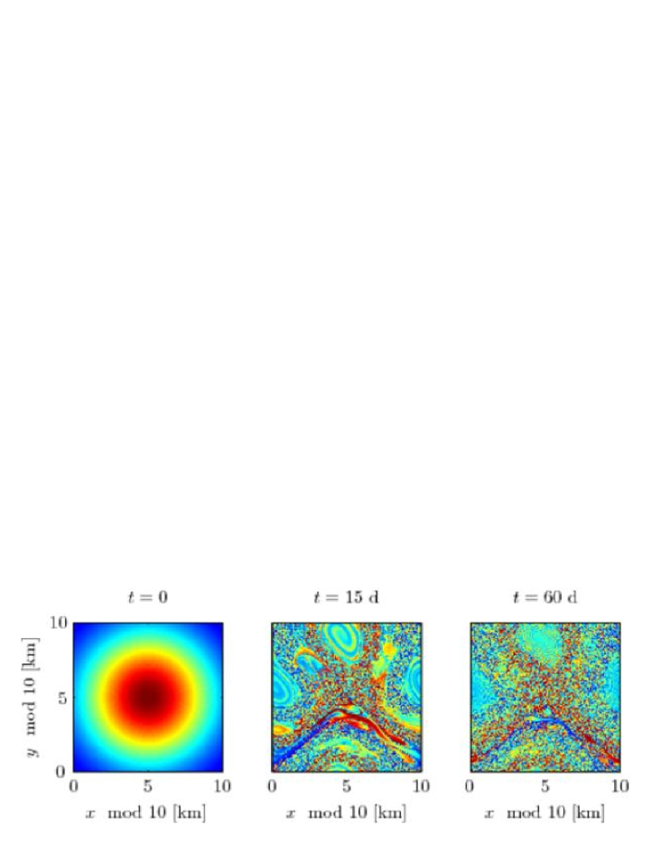
Figure 2: Snapshots of the evolution of a tracer that is passively advected by the time-quasiperiodic tidal velocity field defined by streamfunction (2.1) with the same parameters used to construct the Poincaré section in the right panel of Fig. 1. The color scale indicates tracer concentration or simply a fluid particle labeling.

Fig. 2 illustrates the above for an arbitrary tracer that is passively advected by the quasiperiodic tidal current defined by streamfunction (2.1) with parameters as in Fig. 1. To construct Fig. 2 we advected $250000$ fluid particles distributed initially over a regular grid defined on a doubly-periodic $10$ km $\times$ $10$ km domain of ${\mathds{R}\/}^{2}$. The spatial distribution of the tracer at any stage of the evolution is obtained from Delaunay triangulation of fluid particle positions by triangle-based cubic interpolation onto the regular grid. The distribution of the tracer at $t=0$ is assumed to be a Gaussian. At $t=15$ d the tracer distribution reveals vigorously stirred regions along with poorly stirred regions in the form of spiral-like vortices and filaments. These features resemble quite closely those embodying the mixed phase space shown in the right panel of Fig. 1. The mixed phase-space features are much more clearly visible in the tracer distribution at the later instant $t=60$ d, which can be considered long enough for (constrained) chaotic stirring to develop substantially. Note, however, that $60$ d is much shorter than the integration time required to construct the second-order Poincaré section in the right panel of Fig. 1.

An important observation is that the tracer distribution features can never match those of the mixed phase space because, as explained above, the mixed phase space features “dance” with the “rhythm” of the quasiperiodic tide. This contrasts with the standard chaotic advection paradigm (time-periodic $\psi$) for which the motion of the mixed phase space structures is periodic. In that case matching can be achieved by displaying the tracer distribution at some (sufficiently large) multiple of the time-period of $\psi$.

4 Biologically Interacting Passive Tracer Dynamics

This section is devoted to show that Lagrangian mixed phase-space dynamics can play a distinguished role in setting the distribution of biologically interacting tracers depending on the nature of the interaction. We will assume that the biologically interacting tracers obey a coupled set of Liouville equations of the form

$$\partial_{t}\theta+[\theta,\psi]=F_{\theta}(\theta,t),$$ (4.1)

where $\theta$ is understood as a vector of biologically interacting tracers and $F_{\theta}(\theta,t)$ represents the interaction. The solution of (4.1) may be expressed as

$$\theta(x,y,t)=\theta_{\mathrm{rest}}(\phi_{0,-t}(x,y),t),$$ (4.2)

where $\theta_{\mathrm{rest}}(x,y,t)$ is the solution of (4.1) with initial distribution $\theta_{\mathrm{rest}}(x,y,0)=\theta(x,y,0)$ assuming that the fluid is at rest. In other words, the distribution of $\theta$ at time $t$ is given by an area-preserving rearrangement of the distribution it would have attained at that same instant if the fluid were at rest.

Our particular focus will be on the plankton distribution problem, which we will approach by considering the interaction between phytoplankton, $P$, and zooplankton, $Z$, in a two-level food chain. We will consider nonautonomous Rosenzweig–MacArthur [35] predator–prey interactions governed by

$$F_{P}(P,Z,t)=r(t)\left(1-\frac{P}{K(t)}\right)P-\frac{cPZ}{P_{\mathrm{s}}+P},$$ (4.3a)

$$F_{Z}(P,Z,t)=\frac{ecPZ}{P_{\mathrm{s}}+P}-dZ,$$ (4.3b)

where

$$r(t)=r_{0}(1-\epsilon\cos\Omega t),\quad K(t)=K_{0}(1-\epsilon\cos\Omega t).$$ (4.4)

In this model the prey density, $P$, grows logistically with growth rate $r(t)>0$ and carrying capacity $K(t)>0$ in the absence of predation, $Z=0$. The predator consumes the prey according to a Holling’s type-II functional response, which presumes a maximal consumption rate $c>0$ and half-saturation density $P_{\mathrm{s}}>0$. The model further assumes that the predator’s per capita death rate, $d>0$, is independent of density, and that its numerical response is proportional to its functional response with efficiency $e>0.$ We will set $2\pi/\Omega=1$ d so that (4.4) crudely accounts for the diurnal cycle of light availability.

Other, more sophisticated and perhaps more realistic, two- or higher-level food chain models and multispecies systems have been proposed, which could of course be considered. However, model (4), while very simple, describes a very rich variety of biological interaction types, which is enough for the purposes of the present work.

4.1 Biological Interactions

The predator–prey interactions governed by (4), i.e., $\dot{P}=F_{P}(P,Z,t)$ and $\dot{Z}=F_{Z}(P,Z,t)$ along $(x(t),y(t))$, constitute a dissipative dynamical systems provided $P_{\mathrm{e}}/K\neq 0$ and $P_{\mathrm{e}}/P_{\mathrm{s}}\neq 0,$ where

$$P_{\mathrm{e}}:=\frac{dP_{\mathrm{s}}}{ec-d},$$ (4.5)

which is biologically most sensible. Consequently, the topology of phase space for predator–prey interactions will be fundamentally different than the topology of phase space for fluid particle motion governed by (2.3) and discussed in Section 2. Predator–prey interactions are described in the next paragraph; for a more detailed description the reader is referred to Refs. [36, 37].

In the autonomous case ($\epsilon=0$), predator–prey interactions obeying (4) possess a unique positive equilibrium $(P_{\mathrm{e}},Z_{\mathrm{e}}),$ where

$$Z_{\mathrm{e}}:=\frac{r_{0}}{c}\left(1-\frac{P_{\mathrm{e}}}{K_{0}}\right)\left(P_{\mathrm{s}}+P_{\mathrm{e}}\right),$$ (4.6)

provided $0\leq P_{\mathrm{e}}/K_{0}<1$ and $P_{\mathrm{e}}/P_{\mathrm{s}}\geq 0$. This equilibrium is subject to a change of stability type through a Hopf bifurcation. For $P_{\mathrm{e}}/K_{0}>1/(2+P_{\mathrm{s}}P_{\mathrm{e}})$ predator and prey densities undergo damped oscillations toward $(P_{\mathrm{e}},Z_{\mathrm{e}})$, while for $P_{\mathrm{e}}/K_{0}<1/(2+P_{\mathrm{s}}/P_{\mathrm{e}})$ predator and prey densities experience time-asymptotic, self-sustained oscillations about $(P_{\mathrm{e}},Z_{\mathrm{e}})$.

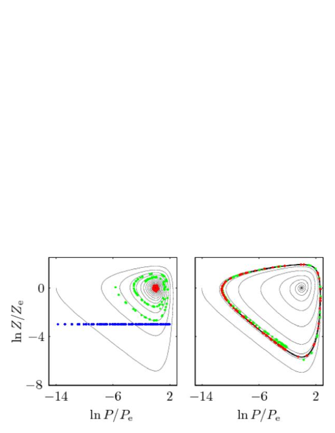
Figure 3: Phase portraits for phytoplankton, $P$, and zooplankton, $Z$, interacting according to autonomous predator–prey dynamics governed by (4), i.e., with $\epsilon=0$ in (4.4). The thin-solid curve in the right panel depicts a damped oscillation toward $(P_{\mathrm{e}},Z_{\mathrm{e}})$, defined in Eqs. (4.5)–(4.6), for $\ln P_{\mathrm{e}}/K_{0}=-3$ and $\ln P_{\mathrm{e}}/P_{\mathrm{s}}=-4$. The thick-solid closed curve in the left panel illustrates a self-sustained oscillation about the equilibrium $(P_{\mathrm{e}},Z_{\mathrm{e}})$ for $\ln P_{\mathrm{e}}/K_{0}=-2.8$ and $\ln P_{\mathrm{e}}/P_{\mathrm{s}}=-1.6$; orbits for two different initial conditions are shown in this panel as thin-solid curves, which collapse into the limit cycle represented by the thick-solid curve. In both panels $r_{0}/\Omega=0.4475$ and $d/\Omega=0.2011.$ The blue dots in the left panel correspond to a discrete set of $P$–$Z$ values in the range spanned by the distributions shown in Figs. 5–6 at $t=0$. The green (resp., red) dots in the left and right panels correspond to a discrete set of $P$–$Z$ values in the range spanned by the distributions shown, respectively, in the top and mid-top row panels of Figs. 5–6 at $t=15$ d (resp., $t=60$ d).

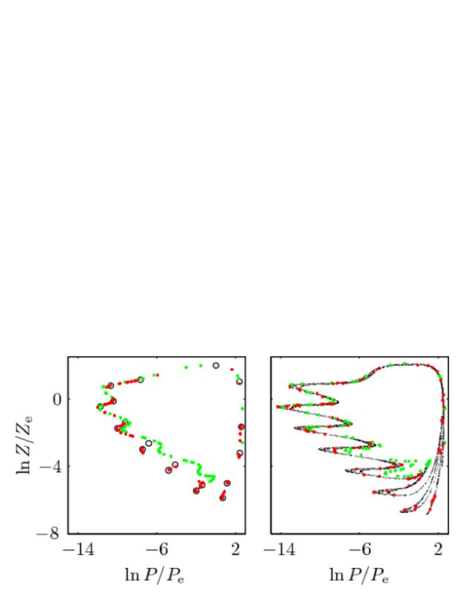
Figure 4: As in Fig. 3, but for nonautonomous predator–prey dynamics governed by (4), i.e., with $\epsilon\neq 0$ in (4b). The left and right panels correspond to Poincaré sections showing, respectively, a periodic attractor ($1:18$ subharmonic) attained with $\epsilon=0.2$ and a strange attractor attained with $\epsilon=0.6;$ in both panels $\ln P_{\mathrm{e}}/K_{0}=-2.8$, $\ln P_{\mathrm{e}}/P_{\mathrm{s}}=-1.6$, $r_{0}/\Omega=0.4475$, and $d/\Omega=0.2011.$ The green (resp., red) dots in the left and right panels correspond to a discrete set of $P$–$Z$ values in the range spanned by the distributions shown, respectively, in the mid-bottom and bottom row panels of Figs. 5–6 at $t=15$ d (resp., $t=60$ d).

In the nonautonomous case ($\epsilon>0$), the equilibrium $(P_{\mathrm{e}},Z_{\mathrm{e}})$ is replaced by a small-amplitude periodic orbit that loses stability through discrete Hopf or Neimark–Sacker bifurcations. Chaotic predator–prey interactions, which are characterized by the presence of a strange attractor, eventually give rise via either torus destruction (quasiperiodic route to chaos) or a cascade of period doublings (subharmonic route to chaos). The first kind of strange attractors results for small $\epsilon$ when the autonomous predator–prey interactions lie on a limit cycle. Strange attractors of the second class develop for larger $\epsilon$, even when the autonomous predator–prey system does not cycle.

Fig. 3 depicts phase portraits for autonomous interactions that decay toward a stable spiral equilibrium (left panel) and asymptotically cycle (right panel). Fig. 4 shows phase portraits for nonautonomous interactions taking place on a periodic $1:18$ subharmonic attractor (left panel) and lying on a strange attractor attained via quasiperiodic route (right panel). The latter are shown on Poincaré sections of the predator–prey system, which are computed by strobing orbits at the environmental variability frequency $\Omega/2\pi$. To construct Figs. 3–4 the predator–prey equations were numerically integrated using the Dormand–Prince 5(4) algorithm. The period of the limit cycle oscillation in the right panel of Fig. 3 is of about $9$ d. Estimated Lyapunov exponents scaled by $\Omega$ for the strange attractor in the right panel of Fig. 4 are $\{+0.0239,0,-0.0539\}$. This gives a predictability horizon (inverse of the positive Lyapunov exponent) not exceeding 10 d for the chaotic interactions considered here.

Other, intermediate, forms of interaction (not shown but discussed below) are nonautonomous interactions lying on a torus or quasiperiodic attractor, and interactions possessing multiple periodic or quasiperiodic attractors. The former are excited for sufficiently small $\epsilon$ when the autonomous interactions take place on a limit cycle; the latter precede chaotic interactions.

4.2 Biological Interactions and Passive Advection

Figs. 5 and 6 depict, respectively, possible evolution scenarios for phytoplankton and zooplankton, which, while interacting through predator–prey dynamics obeying (4), are passively advected by the same quasiperiodic tidal current involved in the construction of Figs. 1–2. Predator–prey interaction parameters in the top and mid-top row panels of Figs. 5 and 6 are, respectively, as in the left and right panels of Fig. 3. Interaction parameters in the mid-bottom and bottom row panels of Figs. 5 and 6 are, respectively, as in the left and right panels of Fig. 4. Figs. 5–6 were constructed by advecting $250000$ fluid particles, each one carrying phytoplankton and zooplankton densities, distributed on regular grid defined on a doubly-periodic $10$ km $\times$ $10$ km domain of ${\mathds{R}\/}^{2}$ as in Fig. 2. The spatial distributions of phytoplankton and zooplankton at any stage of the evolution are obtained by triangle-based cubic interpolation onto the regular grid based on Delaunay triangulation of the fluid particle positions.

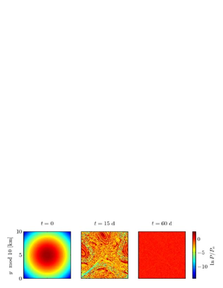
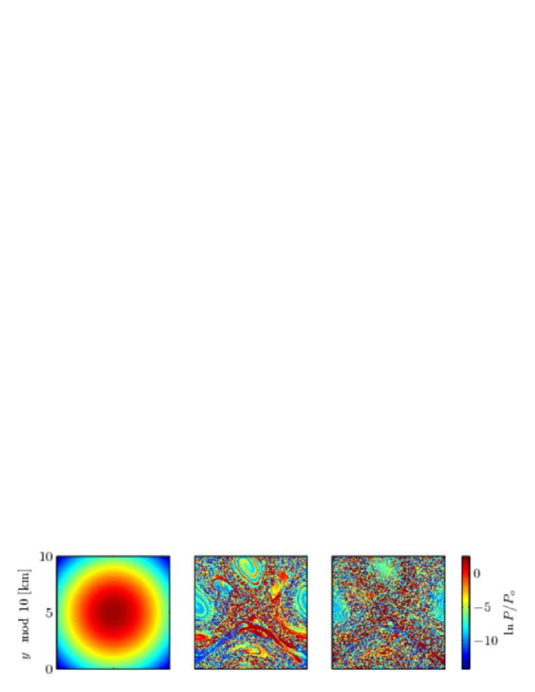
Figure 5: Snapshots of the evolution of phytoplankton, which, while interacting with zooplankton through predator–prey dynamics governed by (4), is advected by the time-quasiperiodic tidal velocity field defined by streamfunction (2.1) with parameters as in the right panel of Fig. 1. Predator–prey interaction parameters in the top and mid-top panels are, respectively, as in the left and right panels of Fig. 3. Parameters in the mid-bottom and bottom row panels are, respectively, as in left and right panels of Fig. 4.

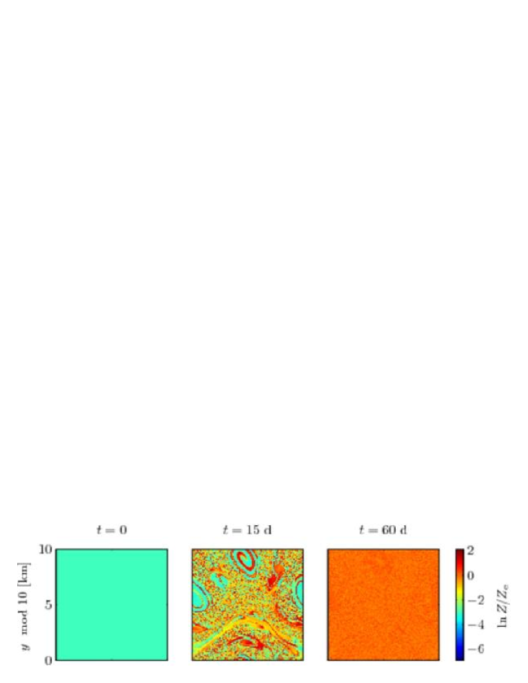
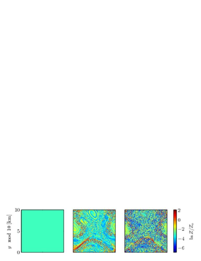
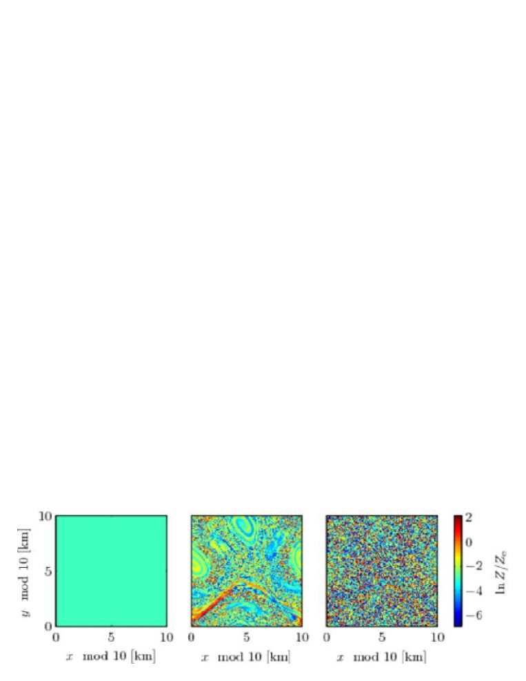
Figure 6: As in Fig. 5, but for zooplankton.

At $t=0$ the phytoplankton distribution (Fig. 5, left column panels) is assumed to be a Gaussian, while the zooplankton distribution (Fig. 6, left column panels) is assumed to be uniform. This corresponds to a sudden (nonuniform) availability of prey resources (phytoplankton blooming) over the entire domain occupied by the predator. The locus in phase space of the initial plankton distributions is indicated by blue dots in Fig. 3–4.

Distributions of phytoplankton and zooplankton after $15$ d (resp., $60$ d) are depicted in the middle (resp., right) column panels of Figs. 5 and 6, respectively. The locus in phase space of these distributions at $t=15$ d (resp., $t=60$ d) is indicated in Figs. 3–4 with green (resp., red) dots. Note that $t=15$ d is still too early for the regular autonomous predator–prey interactions in the left panel of Fig. 3 to reach an asymptotically stable equilibrium, or for the regular nonautonomous predator–prey interactions in the left panel of Fig. 4 to settle on a periodic attracting set. Likewise, at $t=15$ d chaotic predator–prey interactions in the right panel of Fig. 4 produce phytoplankton and zooplankton density values that cover a smaller portion of the corresponding strange attractor than those attained at $t=60$ d. On the other hand, approximately $15$ d must elapse for the autonomous predator–prey interactions in the left panel of Fig. 3 to reach a limit-cycle oscillation.

4.2.1 The Early Evolution Stage

At $t=15$ d phytoplankton (Fig. 5, middle column panels) and zooplankton (Fig. 6, middle column panels) show structures in their distributions that are very similar to those in the distribution of a passive tracer (Fig. 2, middle panel), which are an early manifestation of Lagrangian mixed phase-space dynamics (Fig. 1, right panel). Remarkably, although the estimated predictability horizon for the chaotic predator–prey interactions is shorter than $15$ d, Lagrangian mixed phase-space dynamics shows up very clearly in the plankton distributions. The reason for this is that sensitivity to initial conditions do not manifest at the same time for all orbits emanating from the latter in the phase space for predator–prey interactions. A careful examination of the mid panel in the bottom row of Figs. 5–6, however, reveals small regions of very irregularly distributed plankton interspersed within more uniformly distributed plankton, which are not a result of chaotic stirring but rather of chaotic predator–prey interactions. Other regions of very irregularly distributed plankton resulting from chaotic interactions may lie hidden within the chaotically stirred plankton regions. Clearly, for these regions to get exposed the timescale for substantial development of chaotic stirring must be much larger than the predictability horizon of chaotic predator-prey interactions.

4.2.2 The Late Evolution Stage

At $t=60$ d the regular predator–prey interactions in the left panel of Fig. 3 have almost reached an asymptotically stable equilibrium. Accordingly, the right panel in the top row of Figs. 5 and 6 show very uniformly distributed phytoplankton and zooplankton concentrations, respectively.

At the same instant $t=60$ d, regions of vigorously stirred phytoplankton and zooplankton concentrations along with less stirred regions in the form of filaments and spiral-like vortices develop when regular predator–prey interactions autonomously cycle (Figs. 5–6, right panel in the mid-top row) or nonautonomously behave on a $1:18$ subharmonic attractor (Figs. 5–6, right panel in the mid-bottom row). These features resemble very closely those of the passive tracer distribution at $t=60$ d in the right panel of Fig. 2, which are a manifestation of the mixed phase-space topology that characterizes Lagrangian dynamics. However, note that for predator–prey interactions lying on the $1:18$ subharmonic attractor phytoplankton and zooplankton concentrations can take at most 18 possible discrete asymptotic values (circles in the left panel of Fig. 4). Consequently, at sufficiently long time these interactions will lead to sharper color contrasts in the plankton distributions than autonomously cycling interactions, for which plankton distributions take continuous distributions.

Finally, $t=60$ d is far beyond the predictability horizon estimated for the chaotic predator–prey interactions in the right panel of Fig. 4. Correspondingly, the distributions of phytoplankton and zooplankton are nearly completely mixed (Figs. 5–6, right panel in the bottom row), which is a result of the exponential divergence in time of initially nearby phytoplankton and zooplankton states rather than of chaotic stirring.

4.2.3 Remarks on Other Interaction Scenarios

We close this section briefly discussing (but not showing) the results for the two relevant intermediate nonautonomous biological interactions scenarios mentioned earlier. These are nonautonomous interactions that take place on a quasiperiodic cycle and nonautonomous interactions lying on multiple periodic or quasiperiodic attractors. The quasiperiodically cycling interaction case is not different than autonomously cycling interactions as these are insensitive to initial conditions. The multiple attractor case, in turn, is similar to the chaotic interaction case at long time because the regular (periodic or quasiperiodic) attracting set reached by phytoplankton and zooplankton densities is sensitive to their initial values.

5 Discussion

Suppose that random velocity field fluctuations of the form $\mathbf{u}^{\prime}=\sqrt{2D}(\eta_{1}(t),\allowbreak\eta_{2}(t))$ are superimposed on $\mathbf{u}=(\partial_{y}\psi,-\partial_{x}\psi)$, e.g., with $\psi$ defined by (2.1). Here $D$ is a constant and $\{\eta_{i}\}$ are Gaussian-white-noise random variables satisfying $\left\langle\eta_{i}\right\rangle=0$ and $\langle\eta_{i}(t)\eta_{j}(\tau)\rangle=\delta_{ij}\delta(t-\tau)$, where the angle brackets denote ensemble average. The expected distribution of a passive tracer, $\left\langle\theta\right\rangle$, satisfies [cf., e.g., 38] the Fokker–Plank (advection–diffusion) equation $\partial_{t}\left\langle\theta\right\rangle+[\left\langle\theta\right\rangle,\psi]=D\Delta\left\langle\theta\right\rangle$ with Fickian diffusivity constant $D$, where $\Delta$ is the Laplacian operator in ${\mathds{R}\/}^{2}$. Because $\mathbf{u}^{\prime}$ is a distribution rather than a regular function, the resulting time-dependent vector field, $\mathbf{u}+\mathbf{u}^{\prime}$, is no longer Hamiltonian—at least in a strict sense. Accordingly, KAM tori become permeable to transport and the resonance islands turn leaky. In the long run, the mixed phase-space structures erode completely, and consequently also the spatial patterns in tracer distributions.

Standard ecological theories of pattern formation [cf., e.g., 39] would approach the plankton distribution problem by replacing (4.1) with diffusion equations coupled by predator–prey dynamics, which is equivalent to considering (4.1) with a Gaussian-white-noise random velocity field. Clearly, this approach cannot result in a correct description of plankton advection by an oscillatory velocity field such as the one considered here because the random velocity field cannot produce Lagrangian mixed phase-space dynamics. Remarkably, it has not been until very recently [17] that standard ecological theories have been explicitly recognized as being incapable of providing an appropriate description of the formation of spatial patterns in the distribution of plankton advected by ocean currents. In [17] advection equations like (4.1) are considered where the biological coupling is similar to the one considered here, except that the carrying capacity is set to continually relax toward a spatially nonuniform prescribed function (parameters are chosen so that the biological interactions always contain an asymptotically stable equilibrium). The velocity field in [17] is a kinematic model for mesoscale turbulence, which is envisioned as a superposition of randomly distributed Gaussian eddies; generation of plankton patchiness is mainly attributed to stirring by this velocity field.

The traditional approach to plankton advection by turbulent ocean currents considers, instead of (4.1), a set of biologically-coupled advection–diffusion equations with eddy diffusivities chosen several orders of magnitude larger than molecular diffusivities. Clearly, this choice leads to a complete erosion of any mixed phase-space signature underlying the advection field at a much faster rate than molecular diffusion. More sophisticated, higher-order Markovian stochastic models have been proposed [40] to account for the observed anomalous (i.e., non-Brownian or non-random-walk) dispersion of passive tracers advected by ocean currents, which we believe is more naturally explained by Lagrangian mixed phase-space dynamics. Higher-order Markov models do not [41] give a satisfactory description of the anomalous dispersion behavior typically observed in the ocean. Other stochastic models based on non-Gaussian (Lévy) statistics have been proposed [42], which result in diffusion-type equations involving fractional partial derivatives. These so-called strange kinetic theories, unlike the higher-order Markovian models, have the anomalous dispersion behavior built in, but their practical utility is still not clear.

The present work provides a basis for an alternative approach to the problem of pattern formation in plankton distributions in the presence of noisy advection fields (i.e., large-scale advection fields with small-scale environmental perturbations superimposed) or in turbulent open ocean environments (e.g., mesoscale turbulence). The advection field in those environments may be decomposed into some mean field plus noisy perturbations (not necessarily small) due to environmental variability. The traditional approach would treat the latter as stochastic. An approach in line with the treatment given in this paper would consist in representing the noisy perturbation field in Fourier space. Namely, through the superposition of many harmonics (e.g., Rossby-wave-like modes in the case of mesoscale turbulence) with random phases and amplitudes selected from some modeled or observed wavenumber spectrum (e.g., plausibly following a power law in mesoscale turbulence). For a given random phase realization, the result is a velocity field with a streamfunction that in practice is of the time-quasiperiodic form (2.3b). This allows for a quasi-deterministic description wherein Lagrangian mixed phase-space dynamics plays a central role.

6 Summary and Conclusions

In this paper we have investigated the effect Lagrangian dynamics on the formation of spatial patterns in the distribution of plankton near the surface of the ocean. Advection is assumed to be provided by a divergence-free two-dimensional oscillatory velocity field. Unlike the standard chaotic advection paradigm, in which case the oscillation of the velocity field is periodic, the oscillation is here assumed to be quasiperiodic, i.e., in the form of a superposition of periodic functions with incommensurate frequencies. We analyzed in some detail the two-frequency case, which is suitable for describing tidal motion in shallow seas dominated by a predominantly semidiurnal regime including the spring-to-neap cycle that results from superposing the semilunar and semisolar tidal constituents. The results, however, apply also when many more frequencies are considered, as would be required to model more complicated (turbulent) advection fields. The evolution of phytoplankton and zooplankton is assumed to be controlled by a set of Liouville (advection) equations coupled by deterministic, spatially homogeneous predator–prey dynamics of the standard Rosenzweig–MacArthur class. In addition to autonomous interactions, we considered nonautonomous interactions by letting the food availability to prey cycle diurnally.

The Lagrangian motion is described by a nonautonomous Hamiltonian system with one degree of freedom. The phase space of this motion, which is the physical space for advection, exhibits a mixed topological structure. This includes regions of chaotic motion, possibly separated by KAM tori (transport barriers), and populated by resonance islands (fluid particle traps). The distribution of a passive tracer is thus seen to include vigorously stirred regions and less stirred patches in the form of filaments and spiral-like vortices identifiable with the features that comprise the mixed phase space. These spatial patterns are subject to a quasiperiodic vibration with basic frequencies given by the frequencies of the time-quasiperiodic velocity field. In the particular case analyzed here, the vibration is in synchrony with the assumed quasiperiodic tidal ebb and flood surpluses. This contrasts with standard chaotic advection in which case such a vibration is periodic.

The extent to which phytoplankton and zooplankton distributions are determined by the Lagrangian mixed phase-space dynamics was shown to depend on the type of predator–prey interactions taking place. We considered in detail four possible interaction types: three regular (autonomous stable-spiraling, autonomous cycling, and nonautonomous lying on a periodic attractor) and one complex (nonautonomous taking place on a strange attractor). For autonomously cycling interactions and nonautonomous interactions lying on a periodic attractor, Lagrangian mixed phase-space dynamics leads to the formation of spatial patterns (patchiness) in the distribution of phytoplankton and zooplankton at all stages of the evolution. For autonomous interactions including an asymptotically stable equilibrium, phytoplankton and zooplankton distributions are determined by the mixed phase-space structures during the early stages of the evolution, before complete homogenization is reached. When the population dynamics is chaotic, the influence of Lagrangian mixed phase-space dynamics is limited to a time interval that is not too long compared to the predictability horizon. Two further relevant nonautonomous biological interactions scenarios were also discussed in the paper. These are nonautonomous interactions taking place on a quasiperiodic cycle and lying on multiple periodic or quasiperiodic attractors. In terms of plankton distributions, the former is not very different than autonomously cycling interactions, whereas the latter is similar to the long-term chaotic interaction case because the regular (periodic or quasiperiodic) attracting set reached by an orbit is sensitive to the initial conditions.

Acknowledgements

We thank I. I. Rypina and I. A. Udovydchenkov for the benefit of many helpful discussions on Hamiltonian dynamics. This work has been supported by NSF (USA) grant CMG-0417425 and PARADIGM NSF/ONR-NOPP (USA) grant N000014-02-1-0370.

References

- [1] R. Pasmanter, Fluid Dyn. Res. 3 (1988) 320.
- [2] J.W. Talbot, Proceedings of the International Symposium on Discharge of Sewage from Sea Outfalls, London, 1974.
- [3] V.I. Arnold, Mathematical Methods of Classical Mechanics, 2nd ed. (Springer, 1989).
- [4] G.M. Zaslavsky, Phys. Rep. 371 (2002) 461.
- [5] H. Aref, J. Fluid Mech. 143 (1984) 1.
- [6] F.J. Beron-Vera, M.J. Olascoaga and M.G. Brown, Nonlin. Proc. Geophys. 11 (2004) 67.
- [7] D.V. Makarov et al., (2005), nlin/0507010.
- [8] M.V. Budyansky, M.Y. Uleysky and S.V. Prants, (2005), nlin/0507020.
- [9] Á. Jorba and C. Simó, SIAM J. Math. Anal. 27 (1996) 1,704.
- [10] Á. Jorba and J. Villanueva, J. Nonlin. Sci. 7 (1997) 427 .
- [11] A.R. Osborne et al., Physica D 23 (1986) 75.
- [12] A.R. Osborne et al., Tellus 41A (1989) 416.
- [13] P.L. Richardson et al., J. Phys. Oceanogr. 19 (1989) 371.
- [14] M.G. Brown and K.B. Smith, J. Phys. Oceanogr. 20 (1990) 139.
- [15] J. Nycander, K. Döos and A.C. Coward, Tellus 54A (2002) 99.
- [16] K.L. Denman and T. Platt, J. Mar. Res. 34 (1976) 593.
- [17] E.R. Abraham, Nature 391 (1998) 577.
- [18] M.A. Bees, I. Mezic and J. McGlade, Math. Comp. Sim. 44 (1998) 527.
- [19] Z. Neufeld et al., Geophys. Res. Let. 29 (2002) 10.1029/2001GL013677.
- [20] A.P. Martin, Progr. Oceanogr. 57 (2003) 125.
- [21] R. Reigada et al., Proc. R. Soc. Lond. 270 (2003) 875.
- [22] J.M.G. Vilar, R.V. Solé and J.M. Rubí, Phys. A 317 (2003) 239.
- [23] A. Scheffer et al., Hydrobiologia 491 (2003) 9.
- [24] J.T.F. Zimmerman, Geophys. Astrophys. Fluid Dyn. 11 (1978) 35.
- [25] J.T.F. Zimmerman, Nature 290 (1981) 549.
- [26] H. Ridderinkhof and J.T.F. Zimmerman, Science 258 (1992) 1,107.
- [27] T.S. Parker and L.O. Chua, Practical Numerical Algorithms for Chaotic Systems (Springer, 1989).
- [28] R.I. McLachlan and P. Atela, Nonlin. 5 (1992) 541.
- [29] M.B. Sevryuk, J. Dyn. Cont. Sys. 1 (1995) 351.
- [30] I.I. Rypina et al., J. Atoms. Sci., submitted, arXiv:physics/0605155 (2006).
- [31] S. Aubry, Solitons and Condensed Matter, edited by A.R. Bishop and T. Schneider, pp. 264–278, Springer, 1978.
- [32] I.C. Percival, Nonlinear Dynamics and the Beam-Beam Interaction, edited by M. Month and J.C. Herrera, pp. 302–310, American Institute of Physics, 1979.
- [33] D. Beigie, A. Leonard and S. Wiggins, Nonlinearity 4 (1991) 775.
- [34] D. Makarov and M. Uleysky, J. Phys. A: Math. Gen. 39 (2006) 489.
- [35] M.L. Rosenzweig and R.H. MacArthur, Am. Nat. 97 (1963) 209.
- [36] S. Rinaldi, S. Muratori and Y.A. Kuznetzov, Bull. Math. Biol. 55 (1993) 15.
- [37] A.A. King and W.M. Schaffer, J. Math. Biol. 39 (1999) 439.
- [38] A. Bazzani, S. Siboni and G. Turchetti, Physica D 76 (1994) 8.
- [39] J.D. Murray, Mathematical Biology (Springer, 1988).
- [40] P.S. Berloff and J.C. McWilliams, J. Phys. Oceanogr. 32 (2002) 797.
- [41] E. Castronovo and P.R. Kramer, Monte Carlo Methods and Applications 10 (2004) 245.
- [42] G.M. Zaslavsky, Physica D 76 (1994) 110.