A Model of Intra-seasonal Oscillations in the Earth atmosphere

Abstract

We suggest a way of rationalizing an intra-seasonal oscillations (IOs) of the Earth atmospheric flow as four meteorological relevant triads of interacting planetary waves, isolated from the system of all the rest planetary waves. Our model is independent of the topography (mountains, etc.) and gives a natural explanation of IOs both in the North and South Hemispheres. Spherical planetary waves are an example of a wave mesoscopic system obeying discrete resonances that also appears in other areas of physics.

Introduction. Concept of mesoscopic systems most often appears in condensed matter physics, e.g, in studying properties of superconductors on a scale comparable with that of the Cooper pairscondensed , of miniaturized transistors on a computer chip, of disordered (glassy, granular) systems, when self-averaging is inefficient and fluctuations or the system prehistory become important. Similar situation occurs also in various natural phenomena – from wave turbulent systems in the Ocean zak4 and Atmosphere, when wave lengthes are compatible with the Earth radius KPR , to medicine med1 , and even in sociology and economics, when finite size of a system (population, sociological group, market) becomes important opinion . Mesoscopic regimes are at the frontier between detailed, dynamical and statistical, self-averaging description of systems. Important observation for finite-size, weakly-decaying wave systems was made in K94 : discrete spacial-time resonances form small isolated clusters of interacting modes without energy exchange between the clusters. Clearly, there is exists relatively short, “threshold” wave, involving into the cluster with size large enough to “penetrate” into region of very short waves, where statistical description, that ignores the resonance discreetness, is valid.

Mathematical problem of finding these clusters in concrete cases is equivalent to solving some systems of high ($\gtrsim 12$) order Diophantine equations on a space of 6-8 variables in big integers K98 . Recently developed algorithms for their analysis KK06-12 allows to find, in particular, all resonance clusters of atmospheric planetary waves, described by the spherical functions $Y_{\ell}^{m}$ with eigenvalues $|m|\leq\ell\leq 50$. It turned out that in this domain, consisting of 2500 spherical eigen-modes $Y_{\ell}^{m}$, there exist only 20 different clusters involving only 103 different modes. Moreover, 15 of these clusters have the simplest “triad” structure, formed by three modes. Importantly, there are only four isolated triads in the domain $0<m,\ell\leq 21$, which is meteorological significant for the problem of climate variability on intra-seasonal scale of about 10-100 days (waves with $\ell>21$ have to short period to play significant role in this problem).

The main physical message of our Letter is that so-called Intra-seasonal Oscillations (IOs) of the Earth atmospheric flow can be rationalized as periodical energy exchange within the above mentioned four isolated triads of the planetary waves. IOs has been firstly have been detected mj1 in the study of time series of tropical wind. Similar processes have been also discovered in the atmospheric angular momentum, atmospheric pressure, etc. Detailed analysis of the current state of the problem is presented in gh3 and references therein; most part of the papers are devoted to the detection of these processes in some data sets, all3 ; all1 and to the reproducing them in computer simulations with comprehensive numerical models of the atmosphere  all . Nevertheless, many aspects of the IOs remain unexplained, e.g. the reason of IOs in the North Hemisphere is supposed to be topography, see e.g. all2 and no reason is given for IOs in the South Hemisphere, there is no known way to predict the appearance of IOs, etc.

Our model considers IOs as intrinsic atmospheric phenomenon, related to a system of resonantly interacting triads of planetary waves, which is an example of wave mesoscopic system. The model is equally applied to the North and South Hemispheres, is independent (in the leading order) of the Earth topography, naturally have the period of desired order and allows to interpret the main observable features of IOs (see Sec. 5).

1. Atmospheric planetary waves. These waves are classically studied in the frame of barotropic vorticity equation on a sphere:  KPR :

$$\partial\triangle\psi\big{/}\partial t+2\,\partial\psi\big{/}\partial\lambda+J(\psi,\triangle\psi)=0\ .$$ (1)

Here $\psi$ is the dimensionless stream-function; velocity ${\bm{v}}=\Omega\,R\,[\bf z\times\bm{\nabla}\psi]$, with $\Omega$ being the angular velocity of the Earth and $\bf z$ – the vertical unit vector; the variables $t,\varphi$ and $\lambda$ denote dimensionless time (in the units of $1/\Omega$), latitude ($-\pi/2\leq\varphi\leq\pi/2$) and longitude ($0\leq\lambda\leq 2\pi$) respectively; $\triangle\psi$ and $J(a,b)$ are spherical Laplacian and Jacobian operators. The linear part of this equation has solutions in the form $A_{j}\,Y_{\ell_{j}}^{m_{j}}(\lambda,\varphi)\exp(i\omega_{j}t)$, $\omega_{j}=-2m_{j}/\ell_{j}(\ell_{j}+1)$. Integer parameters $\ell_{j}$ and $(\ell_{j}-m_{j})\geq 0$ are longitudinal and latitudinal wave-numbers of $j$-mode, they are equal to the number of zeros of the spherical function along the longitude and latitude.

Assuming small level of nonlinearity, $|A_{j}|\ll 1$, we restrict ourselves by resonant interactions only. Under the resonance conditions for three modes: $\displaystyle\omega_{1}+\omega_{2}=\omega_{3}\,,\quad m_{1}+m_{2}=m_{3}\,,$ in which $|\ell_{1}-\ell_{2}|<\ell_{3}<\ell_{1}+\ell_{2},$ and $\ell_{1}+\ell_{2}+\ell_{3}$ is odd, the triad amplitudes $A_{j}(t)$ varies in time according to equations KPR :

$$N_{1}d{A}_{1}/dt = 2\,ZN_{32}\,A_{3}A_{2}^{*},\ N_{2}\,d{A}_{2}/dt=2\,Z\,N_{13}\,A_{1}^{*}A_{3},$$

$$N_{3}d{A}_{3}/dt = 2\,ZN_{21}\,A_{1}A_{2}\,,\quad\mbox{for}\ |A_{j}|\ll 1\ .$$ (2)

Here $N_{j}\equiv\ell_{j}(\ell_{j}+1)\,,\ N_{ij}\equiv N_{i}-N_{j}$, and interaction coefficient $Z$ is an explicit function of wave numbers. This system conserves energy $E$ and enstrophy $H$:

$$E=E_{1}+E_{2}+E_{3}\,,\quad H=N_{1}E_{1}+N_{2}E_{2}+N_{3}E_{3}\,,$$ (3)

where the energy of $j$-mode is $E_{j}\equiv N_{j}|A_{j}|^{2}$.

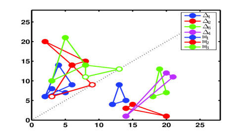
Figure 1: Four isolated triads are shown below the diagonal dash line; $\ell$ – along horizontal axis and $m<\ell$ along the vertical one. The three clusters of two connected triads are shown above diagonal dash line (now $\ell$ – along the vertical axis and $m\leq\ell$ – along the horizontal one). The (meteorological significant) spectral domain is restricted by $0<m,\,\ell\leq 21$. Localized modes are shown by full circles, delocalized ones (with relatively small interaction amplitude) by empty circles.

2. Classification of the triads. Consider the structure and properties of interacting resonant triads in the meteorological significant domain $0<m,\,\ell\leq 21$, where we found four isolated triads, denoted as $\Delta_{1},\dots\,,\Delta_{4}$, three ”butterflies”, i.e. clusters of two triads (denoted as $\bowtie_{1}$, $\bowtie_{2}$ and $\bowtie_{3}$) that are connected by a common mode, and one cluster of 6 connected triads denotes as $\boxtimes$. The structure of all isolated resonant triads and ”butterflies” clusters is shown in Fig. 1. Main information about the triads in the chosen spectral domain is given in left 4 columns on Table 1: notations of the triads, three pair of $\ell_{j},m_{j}$ for each triad, the value of the interaction coefficient $Z$ and the so-called “interaction latitude” $\varphi_{0}$ introduced in Ref. KPR . Columns 5-7 contain data which is necessary to compute period of resonant interactions and will be commented on further.

We can interpret the latitude $\varphi_{0}$ as follows. The overlap of three wave-function in a triad, ${\mathcal{Z}}(\lambda,\varphi)\equiv Y_{\ell_{1}}^{m_{1}}(\lambda,\varphi)Y_{\ell_{2}}^{m_{2}}(\lambda,\varphi)Y_{\ell_{2}}^{m_{3}}(\lambda,\varphi)$ shows a contribution to the interaction coefficient $Z\propto\int{\mathcal{Z}}(\lambda,\varphi)\,d\lambda d\varphi$ from a particular location on the sphere. The overlap ${\mathcal{Z}}(\lambda,\varphi)$

Triad	Modes $[m,\ell]$	$Z$	$\varphi_{0}$	$K[\mu]$	$10^{6}E_{0}$	$T_{0}$
$\Delta_{1}$	[4,12] [5,14] [9,13]	7.82	34	1.62	$14.4$	$24$
$\Delta_{2}$	[3,14] [1,20] [4,15]	37.46	19	1.14	$5.4$	$5$
$\Delta_{3}$	[6,18] [7,20] [13,19]	13.66	34	1.74	$32.0$	$19$
$\Delta_{4}$	[1,14][11,21][12,20]	47.67	28	1.21	$0.58$	$13$
$\bowtie_{1}$	[2,6] [3,8] [5,7]	3.14	35	1.64	$5.08$	$30$
	[2,6] [4,14] [6,9]	14.63	37	1.61	$0.395$	$10$
$\bowtie_{2}$	[6,14] [2,20] [8,15]	69.25	31	1.13	$0.61$	$8$
	[3,6] [6,14] [9,9]	11.31	$-$	1.17	$0.360$	$13$
$\bowtie_{3}$	[3,10] [5,21] [8,14]	61.99	31	1.27	$0.133$	$7$
	[8,11] [5,21] [13,13]	8.71	$-$	1.36	$0.784$	$24$
$\boxtimes$	[1,6] [2,14] [3,9]	28.98	17	1.38	$0.247$	$6$
	[2,7] [11,20] [13,14]	2.77	42	1.08	$1.78$	$26$
	[1,6] [11,20] [12,15]	15.08	29	1.06	$0.262$	$11$
	[9,14] [3,20] [12,15]	74.93	50	1.36	$0.487$	$8$
	[3,9] [8,20] [11,14]	32.12	40	1.11	$0.251$	$9$
	[2,14][17,20][19,19]	11.05	$-$	1.05	$3.33$	$24$

Table 1. For each triad the following data are given: all resonantly interacting modes, interaction coefficient $Z$, interaction latitude $\varphi_{0}$ (in grad), magnitude of the elliptic integral $K(\mu)$, corresponding to the ESMRW December 1989 data for 500 hPa initial energy distribution in a triad, and initial dimensionless energy $E_{0}*10^{6}$ of each triad and resulting $T_{0}$ values (in days).
 
has a maximum at a particular latitude $\varphi_{0}$ and a narrow latitudinal belt around $\varphi_{0}$ gives the main contribution to the global interaction amplitude $Z$. That is why $\varphi_{0}$ can be understood as the interaction latitude.

3. General solution of the triad equations. Linear change of variables $B_{i}=\alpha_{i}A_{i}$ with $\alpha_{i}$ being explicit functions on $N_{j}$ allows to rewrite Sys. (2) as
$\displaystyle~{}~{}~{}\dot{B}_{1}=2ZB_{2}^{*}B_{3},\quad\dot{B}_{2}=2ZB_{1}^{*}B_{3},\quad\dot{B}_{3}=2ZB_{1}B_{2}\ .$
This system has two independent conservation laws

$$I_{1} = |B_{2}|^{2}+|B_{3}|^{2}=(E\,N_{1}-H){N_{23}}/{N_{1}N_{2}N_{3}}\,,~{}~{}~{}~{}$$ (4a)

$$I_{2} = |B_{1}|^{2}+|B_{3}|^{2}=(E\,N_{2}-H){N_{13}}/{N_{1}N_{2}N_{3}}~{}~{}~{}~{}\,,$$ (4b)

which are linear combinations of the energy $E$ and enstrophy $H$. Direct calculations show that the general solution for $B_{i}$ is expressed in Jacobian elliptic functions $B_{1}=B_{1,0}{\rm cn}\,(\tau-\tau_{0})$, $B_{2}=B_{2,0}{\rm sn}\,(\tau-\tau_{0})$, $B_{3}=B_{3,0}{\rm dn}\,(\tau-\tau_{0})$, where $B_{j,0}\,,\ \ \tau_{0}\,,$ are defined by initial conditions and $\tau=t/2\,Z\sqrt[4]{I_{1}I_{2}}\ .$ Functions cn$(\tau)$, sn$(\tau)$ and dn$(\tau)$ are periodic with the period $4K(\mu),4K(\mu)$ and $2K(\mu)$ correspondingly, were $K(\mu)$

$$K(\mu)=\frac{2}{\pi}\int_{0}^{\pi/2}\frac{d\theta}{\sqrt{1-\mu\sin^{2}\theta}}\,,\ \mu^{2}\equiv\min\Big{\{}\frac{I_{1}}{I_{2}}\,,\frac{I_{2}}{I_{1}}\Big{\}}\leq 1\ .$$

Fig 2 illustrates the typical time dependence of all three dimensionless amplitudes of the triad $\Delta_{1}$. One sees that $K(\mu)$ is a smooth function that changes slowly enough such for the wide region of the initial conditions it can be roughly considered as a constant.

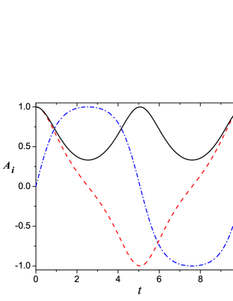
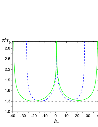
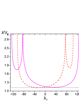
Figure 2: Left panel: Time dependence of $A_{1}$, $A_{2}$ and $A_{3}$ [denoted by green solid, red dashed and blue dot-dashed lines accordingly] of the triad $\Delta_{1}$, with $\mu=0.89$, corresponding to observed data. Middle and Right panels: Dependence of the triad periods $T(E,h)/T_{0}(E)$, Eq. (5a). Middle panel: blue-dashed line corresponds to $\Delta_{1}$ triad, green-solid line – $\Delta_{3}$ triad. Right panel: Red dashed line – $\Delta_{2}$ and magenta solid line – $\Delta_{4}$ triad. Black dashed lines denote minimal period: $T\approx 1.3T_{0}$ for $\Delta_{1}$, $\Delta_{3}$ and $T\approx 1.18T_{0}$ for $\Delta_{2}$, $\Delta_{4}$.

4. Period of triad oscillations. The period of energy exchange (measured in days) in the triads is given by $T={\pi\,K(\mu)}\Big{/}{Z\sqrt[4]{I_{1}I_{2}}}$, that can be written a product of functions $E$ and the ratio of the enstrophy to the energy $h\equiv{H}\big{/}{E}$ :

$$T \ \Rightarrow\ T(E,h)=T_{0}(E)\,K(\mu)\,f(h)\,,$$ (5a)

$$T_{0}(E) = \frac{\pi}{2\,Z\sqrt{2E}}\,\sqrt{\frac{N_{1}N_{2}N_{3}}{N_{21}\sqrt{N_{31}N_{23}}}}\,,~{}~{}~{}~{}~{}$$ (5b)

$$f(h) = \sqrt{N_{12}\big{/}2\sqrt{(N_{1}-h)(h-N_{2})}}\ .$$ (5c)

Here $K$ depends on $\mu$ and, in its turn, $\mu$ depends on $h$ as   $\displaystyle\mu^{2}(h)=\min\Big{[}\ \frac{(h-N_{2})N_{23}}{(N_{1}-h)N_{31}}\,,\frac{N_{1}-h)(N_{31}}{(h-N_{2})N_{23}}\Big{]}$. Equation 3 show that possible values of $h$ lie inside one of the two intervals $N_{2}\geq h\geq N_{1}$ or $N_{1}\geq h\geq N_{2}$. Without loss of generality we set $N_{2}\geq h\geq N_{1}$, then maximal possible value $h=N_{2}$ is realized if $E_{1}=E_{3}=0$, i.e. only the second mode is excited. The minimal value $h=N_{1}$ is possible if $E_{2}=E_{3}=0$, i.e. only the first mode is excited. In both cases, according to basic Eqs. 2 there is no time evolution, i.e. $E_{j}=$ const. for $j=1,2$ and $3$. This is in agreement with Eq. 5c, according to which $f(h)\to\infty$ for $h\to N_{2}$ or $h\to N_{1}$.

Function $f(h)$, Eq. (5c), has a minimum (equal to one) just in the middle of the interval $N_{2}\geq h\geq N_{1}$ at $h=h_{+}\equiv(N_{1}+N_{2})/2$. For this value of $h$ $\displaystyle\hskip 56.9055pt\mu^{2}(h_{+})=\min\Big{\{}\ \frac{(N_{2}-N_{3})}{(N_{3}-N_{1})}\,,\frac{(N_{3}-N_{1})}{(N_{2}-N_{3})}\Big{\}}$. For isolated triads of interest $\Delta_{1}\,,\Delta_{2}\,,\Delta_{3}$ and $\Delta_{4}$ , the values of $\mu^{2}(h_{+})$ are 0.93, 0.41, 0.97 and 0.45 respectively, with $K(\mu)$ equal to 1.96, 1.27, 2.22 and 1.30.

The less trivial case of infinite period corresponds to $\mu=1$, which is realized at $h=h_{\rm crit}\equiv N_{1}+N_{2}-N_{3}$. In this case $B_{3}(\tau)=\tanh\tau$ and for $\tau\to\infty$, $B_{3}\to 1$ and $B_{1}$ and $B_{2}$ exponentially fast go to zero, i.e. for the specific value $h=h_{\rm crit}$, the high mode $B_{3}$ exponentially fast takes energy from two low modes. This is possible only for three particular values of $h$: $h=N_{1}$, $N_{2}$ and $N_{1}+N_{2}-N_{3}$. The $h$ dependence of the period of the triads $\Delta_{1}\,,\dots\,,\Delta_{4}$, is presented in Fig. 2. One sees, that the regions, where the period exceeds twice the minimal possible are very narrow, just few percent of the available interval of $h$. This means, that though theoretically for each triad we can always choose initial conditions in such a way that period will be large and even tend to infinity, the probability of this is very small.

Indeed, for qualitative analysis we can think that in the turbulent atmosphere the probability to get some energy from global disturbances to a particular planetary wave is independent from the state of other waves and this probability is more or less the same for each wave in a triad. If so, the probability ${\mathcal{P}}(h)$ to have initial conditions with some value of $h$ has to be a smooth function of $h$ in the whole available interval $N_{2}\geq h\geq N_{1}$. Roughly speaking, we can approximate ${\mathcal{P}}(h)$ as the constant: ${\mathcal{P}}(h)\simeq 1\big{/}(N_{2}-N_{1})$, $N_{2}\geq h\geq N_{1}$. With this approximation we can, for example, for triads $\Delta_{1}$–$\Delta_{4}$ estimate the probability to have the period, twice exceeding the minimal one $T_{0}(E)$, Eq. (5b), as few percents. Moreover, as one sees in Fig. 2, the typical value of the period $T$ is about $(1.4\pm 0.1)T_{0}$ for the triads $\Delta_{1}$, $\Delta_{3}$ and about $(1.2\pm 0.1)T_{0}$ for the triads $\Delta_{2}$, $\Delta_{4}$. This conclusion is in a qualitative agrement with the ECMWF (European Center for Medium-Range Weather Forcast) winter data, shown in Table 1, column 7.

5. ​​Intra-seasonal ​​Oscillations ​​as ​Resonant ​Triads. Our interpretation of IOs as dynamical behavior of $\Delta_{1}\,,\Delta_{2}\,,\Delta_{3}$ and $\Delta_{4}\$ triads allows one to answer some questions appearing from meteorological observations gh3 .
• What is the cause of IOs in South Hemisphere? The basic fact of our model is the existence of global nonlinear interactions among planetary waves, independent of the topography.
• Why the period of so-called ”topographic” oscillation in North Hemisphere is given as 40 days by some researchers and 20-30 days - by other researchers? The variations in the magnitudes of the period are caused by different initial energy and/or initial energy distribution among the modes of the same triad.
• How do the tropical and mid-latitude oscillations interact? Two mechanisms are possible: i) Triads with substantially different interaction latitudes belonging to the same group, for instance, triads [(1,6) (2,14) (3,9)] and [(3,9) (8,20) (11,14)] of $\boxtimes$ exchange their energies through other modes of this group and belong correspondingly to the tropical and extra-tropical latitudinal belts, and ii) Isolated triads can interact via some special modes called active near-resonant modes K94 . These modes have smallest resonance width with a given triad, and are themselves parts of some other resonant triad. For instance, the mode (13,19) is a near resonant for $\ \Delta_{4}\$ (with resonance discrepancy $\delta=0.16$) and is resonant for $\ \Delta_{3}$.
• Why do the intra-seasonal oscillations are better observable in winter data? In summer, modes have higher energies, periods of the triads become smaller, and resonances with big enough resonance width can destroy the clusters.
• How to predict these recurrent features? Amplitudes of the spherical harmonics with wave numbers taken from Table 1 have to be correlated: $\langle A_{1}(t)A_{2}(t)A_{3}^{*}(t)\rangle\sim\sqrt{\langle|A_{1}(t)|^{2}\rangle\langle|A_{2}(t)|^{2}\rangle\langle|A_{3}(t)|^{2}\rangle}$, see Fig. 2. Magnitudes of the expected periods can be computed beforehand by the given explicit formulae.

6. Conclusions

•  Our simple model provides main robust features of IOs in terms of resonance clusters consisting of three modes of atmospheric waves.

•  Energy behavior within the bigger clusters should be a subject of a special detailed study. Knowledge of cluster structure allows to simplify drastically their analysis. For instance, for ”butterfly” cluster at least 6 real integrals of motions can be easily found. Universal method to construct isolated clusters and write out explicitly corresponding dynamical equations for a wide class of mesoscopic systems is given in KM07 .

•  Our approach is quite general and can be used for studying many other mesoscopic systems, provided that explicit form of dispersion function $\ \omega({\bm{k}})\$ is known (here ${\bm{k}}$ is the wave vector of plane systems with periodical boundary conditions, or another set of eigenvalues in more complicated cases, like $\ m,\ell\$ for the sphere). Properties of a specific mesoscopic system will depend on the 1) form of $\ \omega({\bm{k}})$, 2) dimension of ${\bm{k}},$ 3) number of conservation laws, 4) initial magnitudes of the conserved values (energy, enstrophy, etc.) and their initial distribution among the modes in the cluster.

Acknowledgement. We express our gratitude to Vladimir Zeitlin, anonymous referees and specially to Grisha Volovik for various comments and advises. We are thankful to Yuri Paskover, Oleksii Rudenko and Mark Vilensky for stimulating discussions and help. We also acknowledge the support of the Austrian Science Foundation (FWF) under projects SFB F013/F1301,F1304 and of the US-Israel Binational Science Foundation.

References

- (1) A.K. Geim, I.V. Grigorieva, S.V. Dubonos, J.G.S. Lok, J.C. Maan, A.E. Filippov, F.M. Peeters. Nature 390, 259 (1997)
- (2) V.E. Zakharov, A.O. Korotkevich, A.N. Pushkarev, A.I. Dyachenko. JETP Letters, 82 (8), 491 (2005)
- (3) G.M. Reznik, L.I. Pieterbarg, E.A. Kartashova. Dyn. Atm. Oceans, 18, 235 (1993)
- (4) A. Stefanovska, M.B. Lotric, S. Strle, H. Haken. Physiol. Meas. 22, 535; doi:10.1088/0967-3334/22/3/311 (2001)
- (5) R.Toral, C.J.Tessone. Comm. Comp. Phys. 2 (2), 177 (2007)
- (6) E. Kartashova. Phys. Rev. Let., 72, 2013 (1994)
- (7) E.A. Kartashova. AMS Transl. 182 , 95 (1998)
- (8) E. Kartashova, A. Kartashov: Int. J. Mod. Phys. C 17 1579 (2006); Comm. Comp. Phys. 2 783 (2007); E-print: arXiv.org:math-ph/0701030. To appear in Physics A: Stat. Mech. Appl. doi:10.1016/j.physa.2007.02.098 (2007)
- (9) R.A. Madden, P.R. Julian. J. Atmos. Sci. 28 , 702 (1971)
- (10) M. Ghil, D. Kondrashov, F. Lott, A.W. Robertson. Proc. ECMWF/CLIVAR Workshop on Simulations and prediction of Intra-Seasonal Variability. November 3-6, 2003. Reading, UK (2004), see also extencive bibliogr. therein.
- (11) F.D. Campello, J.M.B. Saraiva, N. Krusche. Atm. Sci. Lett. (5), 65 (2004)
- (12) Ch. A. C. Cunningham, I. F. De Albuquerque Cavalcanti. Int. J. Climatology 26 , 1165 (2006)
- (13) K. Takaya, H. Nakamura. J. Atmos. Sci. 62 , 4441 (2005)
- (14) K. Rajendran, A. Kitoh. J. Climate (19), 366 (2006)
- (15) E. Kartashova, G. Mayrhofer. E-print arxiv.org:nlin/0703039. Submitted to Physica A: Stat. Mech. Appl. (2007)