Generalised Recurrence Plot Analysis for Spatial Data

Abstract

Recurrence plot based methods are highly efficient and widely accepted tools for the investigation of time series or one-dimensional data. We present an extension of the recurrence plots and their quantifications in order to study recurrent structures in higher-dimensional spatial data. The capability of this extension is illustrated on prototypical 2D models. Next, the tested and proved approach is applied to assess the bone structure from CT images of human proximal tibia. We find that the spatial structures in trabecular bone become more self-similar during the bone loss in osteoporosis.

,

1 Introduction

Recurrence is a fundamental property of many dynamical systems and, hence, of various processes in nature. A system may strongly diverge, but after some time it recurs “infinitely many times as close as one wishes to its initial state” [1]. The investigation of recurrence reveals typical properties of the system and may help to predict its future behaviour. With the study of nonlinear chaotic systems several methods for the investigation of recurrences have been developed. The method of recurrence plots (RPs) was introduced by Eckmann et al. [2]. Together with different RP quantification approaches [3, 4], this method has attracted growing interest for both theory and applications [5].

Recurrence plot based methods have been succesfully applied to a wide class of data from physiology, geology, physics, finances and others. They are especially suitable for the investigation of rather short and nonstationary data. This approach works with time series or phase space reconstructions (trajectories), i. e. with data which are at least one-dimensional.

Recurrences are not restricted to one-dimensional time series or phase space trajectories. Spatio-temporal processes can also exhibit typical recurrent structures. However, RPs as introduced in [2] cannot be directly applied to spatial (higher-dimensional) data. One possible way to study the recurrences of spatial data is to separate the higher-dimensional objects into a large number of one-dimensional data series, and to analyse them separately [6]. A more promising approach is to extend the one-dimensional approach of the recurrence plots to a higher-dimensional one.

In the presented work, we focus on the analysis of snapshots of spatio-temporal processes, e. g., on static images. An extension of recurrence plots and their quantification to higher-dimensional data is suggested. This extension allows us to apply this method directly to spatial higher-dimensional data, and, in particular, to use it for 2D image analysis. We apply this method to 2D pQCT human bone images in order to investigate differences in trabecular bone structures at different stages of osteoporosis.

2 Recurrence Plots

The initial purpose of recurrence plots was the visualisation of recurrences of system’s states $\vec{x}_{i}$ in a phase space (with dimension $m$) within a small deviation $\varepsilon$ [2]. The RP efficiently visualises recurrences even for high dimensional systems. A recurrence of a state at time $i$ at a different time $j$ is marked within a two-dimensional squared matrix with ones and zeros dots (black and white points in the plot), where both axes represent time. The RP can be formally expressed by the matrix

$$\mathbf{R}_{i,j}=\Theta\left(\varepsilon-\left\|\vec{x}_{i}-\vec{x}_{j}\right\|\right),\quad\vec{x}_{i}\in\mathds{R}^{m},\quad i,j=1\ldots N,$$ (1)

where $N$ is the number of considered states $\vec{x}_{i}$, $\varepsilon$ is a threshold distance (an arbitrary deviation range within a recurrence is defined), $\|\cdot\|$ denotes a norm and $\Theta(\cdot)$ is the Heaviside function.

It should be emphasised that this method is a pairwise comparison of system’s states at different times along a phase space trajectory, which is – although lying in an $m$-dimensional space – a one-dimensional curve. The axes of the RP correspond to the time which is given by pursueing a state on the trajectory. Diagonal lines in an RP represent epochs of similar dynamical evolution of the analysed system. For $i=j$ we get the line of identity (LOI), $\mathbf{R}_{i,i}\equiv 1\,|_{i=1}^{N}$, which is the main diagonal line in the RP (Fig. 1).

Instead of using the system’s states $\vec{x}_{i}$ which are often unknown, RPs can be created by only using a single time series or a reconstruction of the phase space vectors (e. g. by using time-delay embedding, [7]). Such applications to experimental data have expanded the utilisation of RPs from a tool for the investigation of deterministic phase space dynamics to a tool for the investigation of similarity and transitions in data series, without the rather strong requirement that the data must be from a deterministic dynamical process. The idea of such a similarity plot is not new and can be found in publications earlier than [2], e. g. in [8]. This alternative understanding was (unconsciously) the base of the ever increasing amount of application of RPs in data analysis. However, in its present state the RP technique could not be applied on higher-dimensional spatial data.

The initial purpose of RPs was the visual inspection of the behaviour of phase space trajectories. The appearance of RPs gives hints about the characteristic time evolution of these trajectories [5]. A closer inspection of RPs reveals small-scale structures which are single dots, diagonal lines as well as vertical and horizontal lines (Fig. 1).

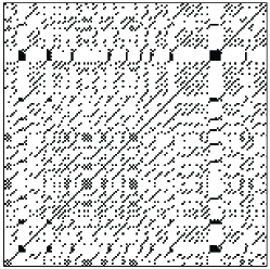
Figure 1: Example of a recurrence plot for the logistic map ($x_{i+1}=ax_{i}(1-x)$ with control parameter $a=3.9767$). The RP consists of single dots and line structures.

A diagonal line $\mathbf{R}_{i+k,j+k}\equiv 1\,|_{k=0}^{l-1}$ (where $l$ is the length of the diagonal line) occurs when one segment of the trajectory runs parallel to another one, i. e. the trajectory re-visits the same region of the phase space at different time intervals. The length of this diagonal line is determined by the duration of intervals with similar local behaviour of the trajectory segments. We define a line in the RP as a diagonal line of length $l$, if it fulfils the condition

$$\left(1-\mathbf{R}_{i-1,j-1}\right)\left(1-\mathbf{R}_{i+l,j+l}\right)\prod_{k=0}^{l-1}\mathbf{R}_{i+k,j+k}\equiv 1.$$ (2)

A vertical (horizontal) line $\mathbf{R}_{i,j+k}\equiv 1\,|_{k=0}^{v-1}$ (where $v$ is the length of the vertical line) marks a time interval in which a system’s state does not change in time or changes very slowly. It looks like the state is trapped for some time, which is a typical behaviour of laminar states [4]. Because RPs are symmetric about the LOI by definition (1), each vertical line has a corresponding horizontal line. Therefore, only the vertical lines are henceforth considered. Combinations of vertical and horizontal lines form rectangular clusters in an RP. We define a line as a vertical line of length $v$, if it fulfils the condition

$$\left(1-\mathbf{R}_{i,j-1}\right)\left(1-\mathbf{R}_{i,j+v}\right)\prod_{k=0}^{v+1}\mathbf{R}_{i,j+k}\equiv 1.$$ (3)

These small-scale structures are used for the quantitative analysis of RPs (known as recurrence quantification analysis, RQA). Using the distributions of the lengths of diagonal lines $P(l)$ or vertical lines $P(v)$, different measures of complexity have been introduced (cf. [5] for a comprehensive review of definitions and descriptions of these measures). Here we generalise the measures recurrence rate $RR$, determinism $DET$, averaged diagonal line length $L$, laminarity $LAM$ and trapping time $TT$ in order to quantify higher-dimensional data. (cf. Tab. 1).

Several measures need a predefined minimal length $l_{min}$ or $v_{min}$, respectively, for the definition of a diagonal or vertical line. These minimal lengths should be as minimal as possible in order to cover as much variation of the lengths of these lines. On the other hand, $l_{min}$ and $v_{min}$ should be large enough to exclude line-like structures which represent only single, non-recurrent states, which may occur if the threshold $\varepsilon$ is chosen too large or if the data have been smoothed too stronlgy before computing the RP.

RQA was successfully applied for example for the detection of transitions in event related EEG potentials [9], the study of interrelations between El Niño and climate in the past [10], the investigation of economic data series [11], of nonlinear processes in electronic devices [12] or the study of transitions in chemical reactions [13]. For a number of further applications see, e. g., [5] or www.recurrence-plot.tk.

Table 1: Generalised recurrence quantification measures for spatial data of dimension $d$ and with $\vec{\imath},\vec{\jmath}\in\mathds{Z}^{d}$. Note that these measures assess recurrence information in terms of length while the original RQA measures quantify it in terms of time.

RQA measure	equation	meaning
recurrence rate	$RR=\frac{1}{N^{2d}}\sum\limits_{\vec{\imath},\vec{\jmath}}^{N}\mathbf{R}_{\vec{\imath},\vec{\jmath}}$	percentage of recurrent states in the system; probability of the recurrence of any state
determinism	$DET_{HS}=\frac{\sum_{l=l_{min}}^{N}l\,P(l)}{\sum_{\vec{\imath},\vec{\jmath}}^{N}\mathbf{R}_{\vec{\imath},\vec{\jmath}}}$	percentage of recurrence points which form diagonal hyper-surfaces; related to the predictability of the system
laminarity	$LAM_{HS}=\frac{\sum_{v=v_{min}}^{N}vP(v)}{\sum_{v=1}^{N}vP(v)}$	percentage of recurrence points which form vertical hyper-surfaces; related to the laminarity of the system
averaged diagonal hyper-surface size	$L_{HS}=\frac{\sum_{l=l_{min}}^{N}l\,P(l)}{\sum_{l=l_{min}}^{N}P(l)}$	related to the prediction length of the system
trapping size	$TT_{HS}=\frac{\sum_{v=v_{min}}^{N}vP(v)}{\sum_{v=v_{min}}^{N}P(v)}$	related to the size of the area in which the system does not change

3 Extension to higher dimensions

Now, we propose an extension of RPs to analyse higher dimensional data. With this step we leave the RPs as a method for investigating deterministic dynamics and focus on its potential in determining similar (recurrent) features in spatial data.

For a $d$-dimensional (Cartesian) system, we define an $n$-dimensional recurrence plot by

$$\mathbf{R}_{\vec{\imath},\vec{\jmath}}=\Theta\left(\varepsilon-\left\|\vec{x}_{\vec{\imath}}-\vec{x}_{\vec{\jmath}}\right\|\right),\quad\vec{x}_{\vec{\imath}}\in\mathds{R}^{m},\ \vec{\imath},\,\vec{\jmath}\in\mathds{Z}^{d},$$ (4)

where $\vec{\imath}$ is the $d$-dimensional coordinate vector and $\vec{x}_{\vec{\imath}}$ is the phase-space vector at the location given by the coordinate vector $\vec{\imath}$. This means that we decompose the spatial dimension of $\vec{x}_{\vec{\imath}}$ and consider each space direction separately, e. g. $\vec{x}_{i_{1},i_{2},\ldots i_{d}}$ for $i_{1}=1,\ldots,N$ but $i_{2},\ldots,i_{d}=\text{const}$. Such vectors are now one-dimensional curves in the $m$-dimensional space. Each of these vectors is pairwisely compared with all others. These individual sub-RPs are the components of the final higher-dimensional RP. The resulting RP has now the dimension $n=2\times d$ and cannot be visualised anymore. However, its quantification is still possible.

Similarly to the one-dimensional LOI given by $\mathbf{R}_{i,j}=1\ \forall\,i=j$, we can find diagonally oriented, $d$-dimensional structures in this $n$-dimensional recurrence plot ($n=2\,d$), called the hyper-surface of identity (HSOI):

$$\mathbf{R}_{\vec{\imath},\vec{\jmath}}\equiv 1\quad\forall\ \vec{\imath}=\vec{\jmath}.$$ (5)

In the special case of a two-dimensional image composed by scalar values, we have

$$\mathbf{R}_{i_{1},i_{2},j_{1},j_{2}}\equiv\Theta\left(\varepsilon-\left\|x_{i_{1},i_{2}}-x_{j_{1},j_{2}}\right\|\right),$$ (6)

which is in fact a four-dimensional recurrence plot, and its HSOI ($\mathbf{R}_{i_{1},i_{2},i_{1},i_{2}}\equiv 1$) is a two-dimensional plane.

4 Quantification of Higher-Dimensional RPs

The known RQA is based on the quantification of the line structures in the two-dimensional RPs. Thus, the definition of higher-dimensional equivalent structures is crucial for a quantification analysis of higher-dimensional RPs.

Based on the definition of diagonal lines, Eq. (2), we define a diagonal squared hyper-surface of size $\vec{l}$ ($\vec{l}=(l,\dots,l),\vec{l}\in\mathds{Z}^{d}$) as

$$\left(1-\mathbf{R}_{\vec{\imath}-\vec{1},\vec{\jmath}-\vec{1}}\right)\left(1-\mathbf{R}_{\vec{\imath}+\vec{l},\vec{\jmath}+\vec{l}}\right)\prod_{\begin{subarray}{c}k_{1},k_{2},\dots,\\ k_{d}=0\end{subarray}}^{l-1}\mathbf{R}_{\vec{\imath}+\vec{k},\vec{\jmath}+\vec{k}}\equiv 1.$$ (7)

In particular, for the two-dimensional case such a diagonal hyper-surface (HS) is thus defined as

$$\left(1-\mathbf{R}_{i_{1}-1,i_{2}-1,j_{1}-1,j_{2}-1}\right)\left(1-\mathbf{R}_{i_{1}+l,i_{2}+l,j_{1}+l,j_{2}+l}\right)\prod_{k_{1},k_{2}=0}^{l-1}\mathbf{R}_{i_{1}+k_{1},i_{2}+k_{2},j_{1}+k_{1},j_{2}+k_{2}}\equiv 1.$$ (8)

The next characteristic structure, the vertical squared HS of size $\vec{v}$ ($\vec{v}=(v,\dots,v),\vec{v}\in\mathds{Z}^{d}$) is defined as

$$\left(1-\mathbf{R}_{\vec{\imath},\vec{\jmath}-\vec{v}}\right)\left(1-\mathbf{R}_{\vec{\imath},\vec{\jmath}+\vec{v}}\right)\prod_{\begin{subarray}{c}k_{1},k_{2},\dots,\\ k_{d}=0\end{subarray}}^{v-1}\mathbf{R}_{\vec{\imath},\vec{\jmath}+\vec{k}}\equiv 1.$$ (9)

Its 2D equivalent is

$$\left(1-\mathbf{R}_{i_{1},i_{2},j_{1}-1,j_{2}-1}\right)\left(1-\mathbf{R}_{i_{1},i_{2},j_{1}+v,j_{2}+v}\right)\prod_{k_{1},k_{2}=0}^{v-1}\mathbf{R}_{i_{1},i_{2},j_{1}+k_{1},j_{2}+k_{2}}\equiv 1.$$ (10)

Using these definitions, we can construct the frequency distributions $P(l)$ and $P(v)$ of the sizes of diagonal and vertical HS in the higher-dimensional RP. This way we get generalised RQA measures $DET_{HS}$, $LAM_{HS}$, $L_{HS}$ and $TT_{HS}$ as defined in Tab. 1, which are now suitable for characterising spatial (e. g. two-dimensional) data.

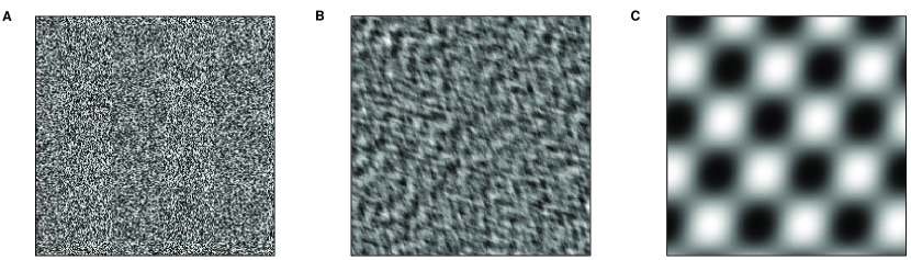
Figure 2: Two-dimensional prototypical examples: test images representing (A) uniformly distributed white noise, (B) a two-dimensional auto-correlated process (2D-AR2) and (C) periodical recurrent structures.

5 Model Examples

In order to illustrate the ability of the proposed high-dimensional RP’s extension, we consider three prototypical model examples from 2D image analysis. The first image (A) is produced by uniformly distributed white noise, the second one (B) is the result of a two-dimensional auto-correlated process of 2nd order (2D-AR2; $x_{i,j}=\sum_{k,l=1}^{2}a_{k,l}\,x_{i-k,j-l}+\xi$, where $a_{k,l}$ is the 2D matrix of model parameters and $\xi$ is Gaussian white noise) and the third one (C) represents periodical recurrent structures (Fig. 2). All these example images have a size of $200\times 200$ pixels and are normalised to a mean of zero and a standard deviation of one.

The resulting RPs are four-dimensional matrices of size $200\times 200\times 200\times 200$, and can hardly be visualised. However, in order to visualise these RPs, we can reduce their dimension by one by considering only those part of the RPs, where $i_{2}=j_{2}$. The resulting $200\times 200\times 200$ cube is a hypersurface of the four-dimensional RP along the LOI. For the threshold we use $\varepsilon=0.2$, which gives clear representations of the RPs.

The features occuring in higher-dimensional RPs provide similar information as known from the classic one-dimensional RPs. Separated single points correspond to strongly fluctuating, uncorrelated data as it is typical for, e. g., white noise (Fig. 3A). Auto-correlations in data cause extended structures, which can be lines, planes or even cuboids (Fig. 3B). Periodical recurrent patterns in data imply periodic line and plane structures in the RP (Fig. 3C). Two-dimensional slices through such RPs contain similar patterns found by common RPs (Fig. 4).

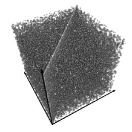
A B C

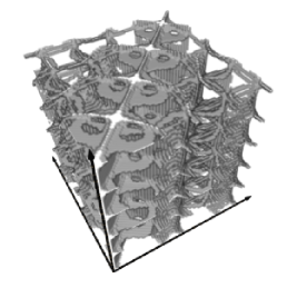
Figure 3: Three-dimensional subsections of four-dimensional RPs of the images shown in Fig. 2. As known from one-dimensional RQA, (A) random data causes homogeneous RPs consisting of single, dis-connected points, (B) correlations in data cause extended connected structures and (C) periodic data induce periodically occuring structures in the RPs.

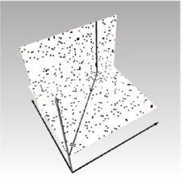
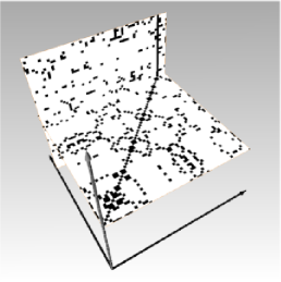
A B C

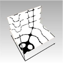
Figure 4: Slices of the subsections of the four-dimensional RPs shown in Fig. 3. The similarity to known recurrence plots is obvious: (A) noise, (B) auto-correlated data and (C) periodic data.

We compute the proposed RQA measures (Tab. 1) for the histograms of the sizes of diagonal and vertical planes (2D HS) in the four-dimensional RPs. For all three examples we use for the minimal size of the diagonal and vertical HS $l_{min}=3$ pixels and $v_{min}=4$ pixels. Although the RQA measures depend on the value of $\varepsilon$, its selection is not crucial for our purpose to discriminate the three different types of structures in the test images. The chosen values for $l_{min}$ and $v_{min}$ are found to be optimal for discriminating the considered images. By choosing smaller values of $l_{min}$ and $v_{min}$ (but larger than one), the measures $DET_{HS}$ and $LAM_{HS}$ are closer for the 2D-AR2 and the periodic image.

Table 2: Recurrence quantification measures for the prototypical examples shown in Fig. 2. The measures are explained in Tab. 1.

Example	$RR$	$DET_{HS}$	$LAM_{HS}$	$L_{HS}$	$TT_{HS}$
(A) noise	0.218	0.007	0.006	3.7	3.0
(B) 2D-AR2	0.221	0.032	0.065	3.1	3.1
(C) periodic	0.219	0.322	0.312	5.8	5.6

Four of five RQA measures clearly discriminate between the three types of images (Tab. 2). Only the recurrence rate $RR$ is roughly the same for all test objects. This is because all images were normalised to the same standard deviation. For the random image (A) the determinism $DET_{HS}$ and laminarity $LAM_{HS}$ tend to zero, what is expected, because the values in the image heavily fluctuate even between adjecent pixels. For the 2D-AR2 image (B), $DET_{HS}$ and $LAM_{HS}$ are slightly above zero, revealing the correlation between adjecent pixels. The last example (C) has, as expected, the highest values in $DET_{HS}$ and $LAM_{HS}$, because same structures occur many times in this image and the image is rather smooth. Although the trend in $DET_{HS}$ and $LAM_{HS}$ is similar, there is a significant difference between both measures. Whereas $LAM_{HS}$ represents the probability that a specific value will not change over spatial variation (what results in extended same-coloured areas in the image), $DET_{HS}$ measures the probability that similar changes in the image recur. $LAM_{HS}$ is twice of $DET_{HS}$ for the 2D-AR2 image, obtaining that there are more areas without changes in the image than such with typical, recurrent changes.

6 Application to pQCT data of proximal tibia

According to the definition of the World Health Organisation, osteoporosis is a disease characterised by bone loss and changes in the structure of the bone. In the last years, the focus changed to structural assessment of the trabecular bone, because bone densitometry alone is very limited to explain all variation in bone strength. Furthermore, the rapid progress in the development of new high-resolution computer tomography (CT) scanners facilitates investigations of the bone micro-architecture. Different approaches using methods coming from nonlinear dynamics have been recently proposed in order to evaluate structural changes [14, 15, 16, 17] or even to predict fracture risks or biomechanical properties [18, 19, 20]. These approaches use, e. g., scaling properties of bone micro-structure or symbol-encoding of the bone architecture.

Using the RP based method, we will focus here on the recurrent structures found in images of trabecular bone of proximal tibiae obtained by peripheral quantitative computer tomography (pQCT). The images were aquired from bone specimens with different stages of osteoporosis as assessed by bone mineral density (BMD). Being applied to such images, the RP provides information about recurrences of bone and soft tissue.

The spatial recurrence analysis is applied to high-resolution pQCT axial slices of human proximal tibia acquired 17 mm below the tibial plateau, with pixel size 200 $\mu$m and slice thickness 1 mm (Fig. 5). The images were acquired from 25 bone specimens with a pQCT scanner XCT-2000 (Stratec GmbH, Germany). The trabecular bone mineral density of these specimens ranges from 30 to 150 mg/cm³. A standardised image pre-processing procedure was applied to exclude the cortical shell from the analysis [15, 21]. The RQA was computed by using the parameters $\varepsilon=0.04$ cm^-1, $l_{min}=v_{min}=400$ $\mu$m. These minimal lengths correspond to two pixels and is found to be appropriate for pQCT images of such resolution.

In order to further evaluate the proposed RQA measures, we compare them with some recently introduced structural measures of complexity (SMCs) [15, 21]. The SMCs are based on a symbol-encoding of bone elements in the pQCT image. Here we focus on the following SMCs:

1. Entropy ($S_{a}$): quantifies the probability distribution of X-ray attenuation within the ROI;

2. Structure Complexity Index (SCI): assesses the complexity and homogeneity of the structure as a whole;

3. Trabecular Network Index (TNI) evaluates richness, orderliness, and homogeneity of the trabecular network.

The computation of the SMCs is applied on the same trabecular area like the RQA measures.

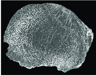
Figure 5: Typical axial pQCT slice of human proximal tibia acquired 17 mm below the tibial plateau. The trabecular BMD is 65.5 mg/cm³.

The application of the recurrence plot extension to the pQCT images of proximal tibiae reveals a relationship between the recurrences in the trabecular architecture and the osteoporotic stage (Fig. 6 and Tab. 3). $RR$ is largest for osteoporotic bone and shows the strongest relationship with the degree of osteoporosis: it is clearly anti-correlated with BMD (Spearman’s rank order correlation coefficient $R=-0.94$). $DET_{HS}$ and $LAM_{HS}$ are also maximal for tibiae with high degree of osteoporosis ($R=-0.66$ and $-0.79$; Fig. 7). We do not find a strong relation between $L_{HS}$, $TT_{HS}$ and BMD. The comparison with the SMCs reveals good relationships between the RQA measures and $S_{a}$, SCI and TNI (Fig. 8 and Tab. 3). Thus, the RQA measures $RR$, $DET_{HS}$ and $LAM_{HS}$ contain also information about the complexity and homogeneity of the trabecular network.

Thus, the proposed RP approach reveals that during the development of osteoporosis the structures in the corresponding pQCT image become more and more recurrent. This is in a good agreement with a decreasing complexity in the micro-architecture of bone. It confirms the results of an analysis of pQCT images acquired from human proximal tibia and lumbar vertebrae based on symbolic dynamics [15, 21]. The direct comparison with the structural quantities (SMCs) shows that the RQA measures provide information about the bone architecture. The RQA measures reveal a low rate of change for bone of higher BMD, but higher rate of changes for specimens with lower BMD (Figs. 6 and 7). This reflects a higher sensitivity of these measures for osteoporotic trabecular bone and emphasises the nonlinear relationship between the bone architecture as assessed by the RQA measures and bone mass as evaluated by the BMD. As it has been recently shown that the SMCs provide a better estimation of the mechanical bone strength than BMD alone [22], the proposed RQA measures could further enhance the evaluation to assess the fracture risk of bone.

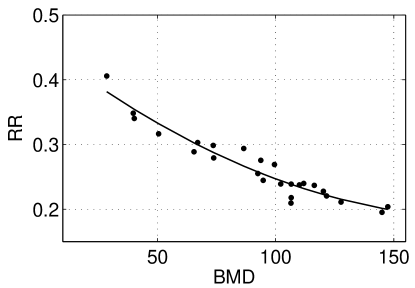
Figure 6: Recurrence rate $RR$ obtained from four-dimensional RPs of pQCT images of trabecular bone in human proximal tibia of different osteoporotic stages.

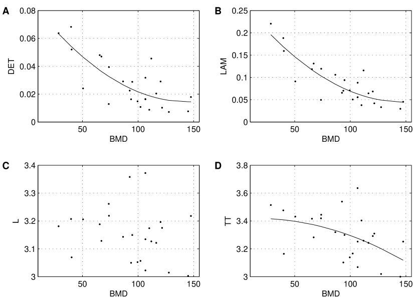
Figure 7: Determinism $DET$ (A), laminarity $LAM$ (B), mean line length $L$ (C) and trapping time $TT$ (D) obtained from four-dimensional RPs constructed from pQCT images of trabecular bone in human proximal tibiae with different degree of osteoporosis.

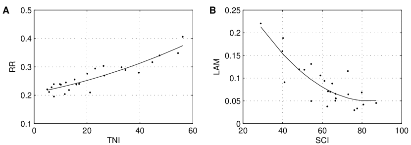
Figure 8: Recurrence rate $RR$ (A) and laminarity $LAM$ (B) compared with trabecular network index TNI and structure complexity index (SCI).

Table 3: Rank correlation coefficients $R$ for recurrence quantification measures, BMD and structural measures of complexity (only significant values are shown).

2D-RQA	BMD	$S_{a}$	SCI	TNI
RR	$-0.94$	$-0.92$	$-0.91$	0.84
DET	$-0.65$	$-0.58$	$-0.61$	0.61
LAM	$-0.78$	$-0.73$	$-0.75$	0.72
L	–	–	–	–
TT	$-0.57$	$-0.51$	–	0.49

6.1 Conclusions

A generalisation of the method of recurrence plots (RPs) and recurrence quantification analysis (RQA) for the application to higher-dimensional spatial data has been proposed here. This new method can be used for 2D image analysis, in particular to reveal and quantify recurrent structures in 2D images. Applying this method on model images, we have shown that it is able to distinguish typical spatial structures by means of recurrences. As a first application, we have used this method for the comparison of CT images of human proximal tibia with different degree of osteoporosis. We have found a clear relationship between some of the proposed RQA measures and the complexity and homogeneity of the trabecular structure. Moreover, this approach can be easily extended to higher dimensions, e. g., for 3D analysis of micro-CT images of human bone. This approach will be the base for the further development of methods for the assessment of structural alteration in trabecular bone with osteoporosis in patients on Earth or in space flying personnel in microgravity conditions.

7 Acknowledgments

This study was supported by grants from project MAP AO-99-030 (contract #14592) of the Microgravity Application Program/Biotechnology from the Human Spaceflight Program of the European Space Agency (ESA) and by the European Union through the Network of Excellence BioSim, contract LSHB-CT-2004-005137&#65533. The authors would also like to acknowledge Scanco Medical AG, Siemens AG, and Roche Pharmaceuticals for support of the study and thank Wolfgang Gowin and Erika May for preparation and scanning of the bone specimens.

References

- [1] H. Poincaré, Sur la probleme des trois corps et les équations de la dynamique, Acta Mathematica 13 (1890) 1–271.
- [2] J.-P. Eckmann, S. O. Kamphorst, D. Ruelle, Recurrence Plots of Dynamical Systems, Europhysics Letters 5 (1987) 973–977.
- [3] C. L. Webber Jr., J. P. Zbilut, Dynamical assessment of physiological systems and states using recurrence plot strategies, Journal of Applied Physiology 76 (2) (1994) 965–973.
-
[4]
N. Marwan, N. Wessel, U. Meyerfeldt, A. Schirdewan, J. Kurths, Recurrence Plot
Based Measures of Complexity and its Application to Heart Rate Variability
Data, Physical Review E 66 (2) (2002) 026702.
URL 10.1103/PhysRevE.66.026702 - [5] N. Marwan, Encounters With Neighbours – Current Developments Of Concepts Based On Recurrence Plots And Their Applications, Ph.D. thesis, University of Potsdam (2003).
-
[6]
D. B. Vasconcelos, S. R. Lopes, R. L. Viana, J. Kurths, Spatial recurrence
plots, Physical Review E 73 (2006) 056207.
URL 10.1103/PhysRevE.73.056207 - [7] F. Takens, Detecting Strange Attractors in Turbulence, Vol. 898 of Lecture Notes in Mathematics, Springer, Berlin, 1981, pp. 366–381.
- [8] J. V. Maizel, R. P. Lenk, Enhanced Graphic Matrix Analysis of Nucleic Acid and Protein Sequences, Proceedings of the National Academy of Sciences 78 (12) (1981) 7665–7669.
-
[9]
N. Marwan, A. Meinke, Extended recurrence plot analysis and its application to
ERP data, International Journal of Bifurcation and Chaos “Cognition and
Complex Brain Dynamics” 14 (2) (2004) 761–771.
URL 10.1142/S0218127404009454 -
[10]
N. Marwan, M. H. Trauth, M. Vuille, J. Kurths, Comparing modern and
Pleistocene ENSO-like influences in NW Argentina using nonlinear time series
analysis methods, Climate Dynamics 21 (3–4) (2003) 317–326.
URL 10.1007/s00382-003-0335-3 - [11] C. G. Gilmore, Detecting linear and nonlinear dependence in stock returns: New methods derived from chaos theory, Journal of Business Finance & Accounting 23 (9–10) (1996) 1357–1377.
-
[12]
A. S. Elwakil, A. M. Soliman, Mathematical Models of the Twin-T,
Wien-bridgeand Family of Minimum Component Electronic ChaosGenerators with
Demonstrative Recurrence Plots, Chaos, Solitons, & Fractals 10 (8) (1999)
1399–1411.
URL 10.1016/S0960-0779(98)00109-X -
[13]
M. Rustici, C. Caravati, E. Petretto, M. Branca, N. Marchettini, Transition
Scenarios during the Evolution of the Belousov-Zhabotinsky Reaction in an
Unstirred Batch Reactor, Journal of Physical Chemistry A 103 (33) (1999)
6564–6570.
URL 10.1021/jp9902708 - [14] C. L. Benhamou, E. Lespessailles, G. Jacquet, R. Harba, R. Jennane, T. Loussot, D. Tourliere, W. Ohley, Fractal Organization of Trabecular Bone Images on Calcaneus Radiographs, Journal of Bone and Mineral Research 9 (12) (1994) 1909–1918.
- [15] P. I. Saparin, W. Gowin, J. Kurths, D. Felsenberg, Quantification of cancellous bone structure using symbolic dynamics and measures of complexity, Physical Review E 58 (5) (1998) 6449.
- [16] W. Gowin, P. I. Saparin, J. Kurths, D. Felsenberg, Measures of complexity for cancellous bone, Technology and Health Care 6 (1998) 373–390.
- [17] G. Dougherty, G. M. Henebry, Fractal signature and lacunarity in the measurement of the texture of trabecular bone in clinical CT images, Medical Engineering & Physics 23 (6) (2001) 369–380.
- [18] T. J. Haire, R. Hodgskinson, P. S. Ganney, C. M. Langton, A comparison of porosity, fabric and fractal dimension as predictors of the young’s modulus of equine cancellous bone, Medical Engineering & Physics 20 (8) (1998) 588–593.
- [19] S. Majumdar, J. Lin, T. Link, J. Millard, P. Augat, X. Ouyang, D. Newitt, R. G. R. M. Kothari, H. Genant, Fractal analysis of radiographs: assessment of trabecular bone structure and prediction of elastic modulus and strength, Med Phys 26 (7) (1999) 1330–1340.
- [20] S. Prouteau, G. Ducher, P. Nanyan, G. Lemineur, L. Benhamou, D. Courteix, Fractal analysis of bone texture: a screening tool for stress fracture risk?, European Journal of Clinical Investigation 34 (2) (2004) 137–142.
- [21] P. Saparin, W. Gowin, D. Felsenberg, Comparison of bone loss with the changes of bone architecture at six different skeletal sites using measures of complexity, Journal of Gravitational Physiology 9 (1) (2002) 177–178.
- [22] P. I. Saparin, J. S. Thomsen, G. Beller, W. Gowin, Measures of complexity to quantify bone loss and estimate strength of human lumbar vertebrae: comparison of pqct image analysis with bone histomorphometry and biomechanical tests, Journal of Gravitational Physiology 12 (1) (2005) 121–122.